Determination of Pollution Loads in Spillways of the Combined Sewage Network of the City of Cuenca, Ecuador

Abstract

Combined sewer overflow (CSO) is one of the main causes of contamination in receiving bodies during the rainy period. The objective of this research was to evaluate the behavior of three combined sewage discharges into the Tomebamba River in the city of Cuenca, Ecuador. For this, the registration of 18 CSO events was carried out. The following water quality parameters were analyzed from the field survey (March 2017 to May 2018): conductivity, turbidity, BOD₅, COD, fecal and total coliforms, nitrates, nitrites, ammoniacal nitrogen, dissolved orthophosphate and total phosphorus. The results show that CSOs contribute to the deterioration of the water quality of the Tomebamba River during the rainy season. The analysis of the dynamics of the pollutants determined that the maximum conductivity values occur at the beginning of the discharge, and the maximum turbidity is located near the peak discharge flow. The relationship between rain and the characteristics of the CSO was also analyzed through a canonical correlation analysis and partial least squares regression, obtaining a prediction model of pollutants based on the precipitation parameters. These results can be used for the implementation of integrated ecological models that enable a complete analysis of the city’s sanitation systems, their impact on the receiving bodies and their restoration.

1. Introduction

In several cities around the world, wastewater and urban runoff water are transported through the same sewage network called the combined sewage network (CSN). Generally, the CSN conducts the flow to a wastewater treatment plant (WWTP) and then returns it to a receiving body. During intense rainfall events, the flow rates in the CSN can greatly exceed the capacity of the WWTP, so structures that allow the discharge of water without any treatment directly into the receiving body are built [1,2,3,4]. This process is called combined sewer overflow (CSO). CSO events have a significant influence on the degradation of the water quality of the receiving bodies during the wet season [2,5,6,7,8,9].

Urban wastewater is mainly composed of organic matter, which causes reduced oxygen levels [10,11]. Additionally, this water contains an important load of microorganisms, most of which are pathogens responsible for transmitting water diseases [10]. On the other hand, runoff waters may contain suspended solids, microorganisms, organic matter, pesticides and metals, depending on their type [11]. The quality of the water that overflows during CSO events varies within the same storm event and between storms [12] and also depends on the characteristics of the rain [2,13,14].

There are several investigations into the effect of CSO processes on water bodies. These evaluate the physical, chemical and biologic characteristics. Some studies examine specific parameters, such as dissolved oxygen [6,15]. Instead, other researchers analyze a larger set of chemical parameters, such as biochemical oxygen demand (BOD₅), chemical oxygen demand (COD), conductivity, pH, ammonium, nitrates and nitrites [8,16,17,18]. Microbiological parameters are also analyzed to determine the quality of the water during CSO [2,5,7,8].

Some researchers analyzed the relationship between rainfall events and CSO characteristics. Yu et al. [3] studied the relationship between CSO characteristics, such as frequency, duration, total volume discharged and average response time and the parameters of rainfall, such as precipitation height, maximum hourly intensity and duration. Mailhot et al. [13] evaluated 4285 combined sewer discharge structures and developed an approach to estimate the average number of CSO events in any one year.

Few authors have investigated the relationship between the precipitation variables and water quality characteristics of CSOs [14,19,20]. Sandoval et al. [14] evaluated the main CSO in Berlin (Germany) through the use of multivariate statistical methods and online measurements. As a result, it was determined that the maximum and average rainfall intensities are the most influential variables to describe the amount of water and the pollutant loads of CSOs, while the duration of the rain event and the depth of the rain seem to be the most influential variables to describe the concentrations of pollutants.

Since 1984, the Water Supply and Wastewater Management Municipal Company ETAPA-EP has implemented several projects to improve the water quality status of the rivers that cross the city of Cuenca. These projects have included the construction of the Ucubamba Wastewater Treatment Plant (U-WWTP), the expansion of the combined sewage network and the construction of sewage interceptors [21]. The operation of these interceptors facilitates recovery of the biologic conditions of the Tomebamba River in the sections located within the urban area of the city of Cuenca [22].

Despite the contribution of the interceptors and the U-WWTP in improving the water quality of the rivers of Cuenca, the discharge of large polluting loads during heavy rainfall events cannot be avoided [23]. The main cause of pollution in the Tomebamba River during the rainy season is sewage that directly discharges into the river without any prior treatment [24]. On many occasions, the achievements made through the construction of treatment plants and the treatment of water in dry weather are invalidated by this type of discharge [25].

The behavior of CSOs has not been studied in detail in Ecuador. In this country, there is currently no legislation directly related to CSO processes. There are only restrictions concerning the discharge of pollutants into receiving water bodies, which merely limit their concentrations [26]. It is also necessary to determine a limit for the total contributions of a pollutant load through the characterization of other related parameters of a CSO. For example, Canadian regulations require municipalities to demonstrate that new developments will not result in an increase in the frequency of CSO. For this, it is recommended to integrate land surface planning with projects to limit overall runoff [13,27].

The aim of this study was to evaluate the behavior of three spillways of the combined sewer system that discharges into the Tomebamba River in the city of Cuenca, Ecuador, through the registration of 18 CSO events from March 2017 to May 2018. This study focuses on a characterization of the pollutant load and its impact on the receiving body. The temporal variability of the polluting parameters during the discharge process is also analyzed; this aspect allows to visualize and to understand the dynamics of pollutants. In addition, the relationships between the rainfall variables and the water quality parameters in the CSOs are determined through the use of multivariate statistical methods. Canonical correlation analysis (CCA) was used to establish the associations between the variables and partial least squares regression (PLSR) was used to develop prediction models that can determine the concentrations of pollutants in the CSOs from precipitation parameters. These models constitute a useful tool that can be used in the implementation of integrated ecological models for the analysis of the city sanitation systems, their impact on the receiving bodies and their restoration. None of these aspects has been studied before with regard to the CSOs of Ecuador.

2. Materials and Methods

2.1. Study Area

The study area includes three urban micro-basins within the city of Cuenca, the capital of the province of Azuay, Ecuador. Cuenca is located in the southern part of the Andean mountains, in the geomorphological zone cataloged as the inter-Andean valley, located at an altitude that varies from 2300 to 2900 m ASL, expanding in a surface of 36 km². The annual average temperature changes, according to the altitude, from 9 to 16.3 °C [28,29]. The rainy season runs from the middle of February until the beginning of July and from the second half of September until the first two weeks of November, while the rest of the year constitutes the dry season [24]. The average rainfall is approximately 879 mm per year [30].

The estimated population in the urban area of Cuenca in 2020 is 407,000 inhabitants [31]. The city is crossed by four main water bodies: The Tomebamba, Yanuncay, Tarqui and the Machángara Rivers. Most contamination in the Tomebamba and Yanuncay Rivers is due to urbanization. On the other hand, in the Machángara River, contamination is also due to industrial discharge. Pollution in the Tarqui River is due to both urbanization and livestock activities in its valleys [24].

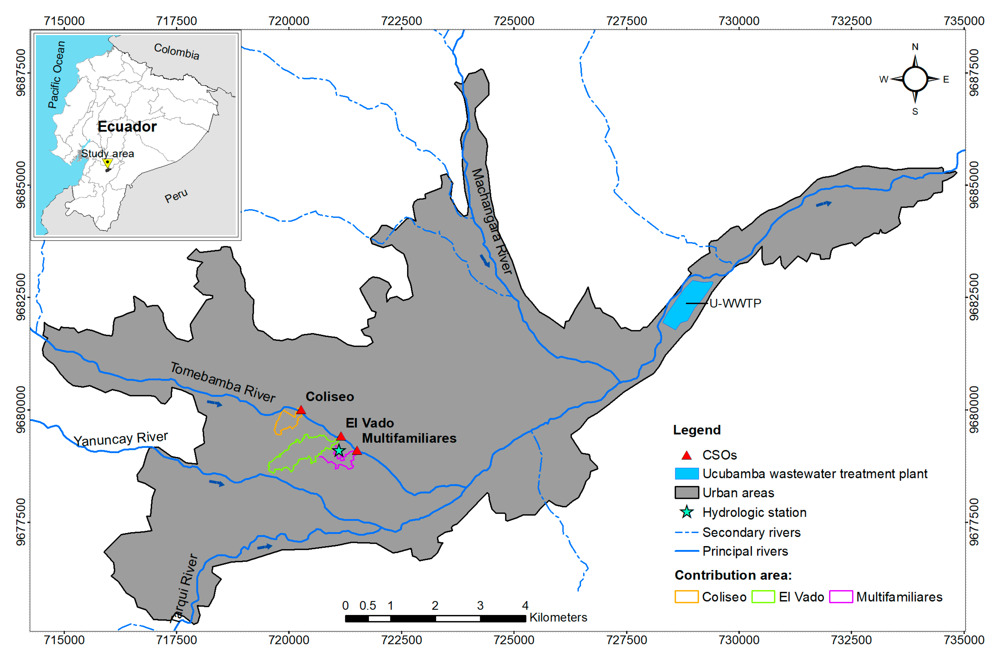
The drainage system of the city of Cuenca consists of approximately a 1300-km sewerage network and an 80-km interceptor network, the latter leading the flow to the Ucubamba wastewater treatment plant (U-WWTP). This plant constitutes the main wastewater treatment infrastructure for the city [22]. The U-WWTP covers an area of approximately 45 hectares and is located at a distance of two kilometers downstream from the confluence of the Machángara with the Tomebamba River (Figure 1). The U-WWTP treats approximately an average flow of 1.2 m³/s [32] and has been in operation since November 1999 [33]. About 80% of the wastewater in the City of Cuenca is treated before its return to the water bodies [22].

The three combined sewerage discharges analyzed in this document are located on the right bank of the Tomebamba River near the city center (Figure 1). The first CSO is called Coliseo, which covers a contribution area of around 18.1 ha. The El Vado CSO is located downstream at approximately 1100 m, and its contribution area reaches 56.0 ha. Finally, 500 m downstream from the latter aforementioned CSO is the Multifamiliares, whose contribution area is 19.4 ha.

During this investigation, a total of 18 CSO events were registered, three in the Coliseo CSO, nine in the El Vado CSO and six in the Multifamiliares CSO. The samplings were carried out during the period from March 2017 to May 2018.

2.2. Discharge Flow Measurement

Flow rates at the discharge points were determined using the section–slope relationship method [34] through the automatic measurement of the water level and a characterization of the uniform flow presented in the approach section near the discharge. The recording of water height was carried out at one-minute intervals using a level sensor connected to an ISCO 6712 probe [20]. Based on the flow height data and information on the geometric and hydraulic characteristics of the pipeline, the discharge hydrograph was determined for each CSO event (Figure 2).

2.3. Sample Collection

Parallel to the flow registration, the samples to determine the water quality parameters were collected.

Table A1. Summary of the collected physical, chemical and microbiological data based on the registration of 18 CSO events in the Coliseo, El Vado and Multifamiliares CSOs in 2017 and 2018.

CSO	Parameter	Units	Mean Value		Standard Deviation	Min Value	Max Value	Median Value
Coliseo	Conductivity	µS/cm	155	±	56	68	295	133
	Turbidity	NTU	216	±	106	68	378	171
	Five-day biochemical oxygen demand	mg/L	170	±	33	140	206	164
	Chemical oxygen demand	mg/L	420	±	327	90	1450	380
	Fecal coliforms	NMP/100 mL	${4.7\times 10}^9$	±	${5.5\times 10}^9$	${1.0\times 10}^9$	${1.4\times 10}^{10}$	${1.1\times 10}^9$
	Total coliforms	NMP/100 mL	${9.0\times 10}^9$	±	${5.5\times 10}^9$	${1.1\times 10}^9$	${2.0\times 10}^{10}$	${1.0\times 10}^{10}$
El Vado	Conductivity	µS/cm	195	±	114	59	616	154
	Turbidity	NTU	131	±	62	47	319	117
	Five-day biochemical oxygen demand	mg/L	93	±	116	7	361	45
	Chemical oxygen demand	mg/L	249	±	149	46	670	240
	Fecal coliforms	NMP/100 mL	${3.6\times 10}^9$	±	${6.0\times 10}^9$	${1.6\times 10}^6$	${1.9\times 10}^{10}$	${3.9\times 10}^8$
	Total coliforms	NMP/100 mL	${6.2\times 10}^9$	±	${6.0\times 10}^9$	${9.8\times 10}^6$	${4.1\times 10}^{10}$	${1.6\times 10}^9$
	Nitrate-N	mg/L	0.26	±	0.16	0.12	0.53	0.22
	Nitrite-N	µg/L	34.7	±	29.1	3.7	66.3	39.3
	Ammoniacal nitrogen—N	mg/L	1.34	±	0.74	0.49	2.54	1.25
	Dissolved orthophosphate—P	mg/L	0.49	±	0.30	0.13	1.03	0.52
	Total phosphorus	mg/L	3.77	±	1.21	2.47	5.65	3.32
Multifamiliares	Conductivity	µS/cm	198	±	112	50	664	183
	Turbidity	NTU	96	±	76	9	345	66
	Five-day biochemical oxygen demand	mg/L	134	±	187	8	528	46
	Chemical oxygen demand	mg/L	262	±	296	40	1410	140
	Fecal coliforms	NMP/100 mL	${3.3\times 10}^9$	±	${3.7\times 10}^9$	${3.5\times 10}^6$	${1.0\times 10}^{10}$	${2.5\times 10}^9$
	Total coliforms	NMP/100 mL	${1.7\times 10}^{10}$	±	${3.7\times 10}^9$	${4.8\times 10}^6$	${4.0\times 10}^{10}$	${1.1\times 10}^{10}$

presents a summary of the data collected from the monitoring of the CSOs. The sampling and measurement of water levels were carried out with the ISCO 6712 automatic equipment and its integrated pumping system [20].

Since there is also precipitation that does not generate sewer overflow, it is necessary to define the threshold above which a CSO event is considered. The definition of this threshold is related to the influence of the overflow on the water quality of the river. If the overflow is slight, the dilution effect of the contaminants is negligible; therefore, it is not considered a CSO event [8]. In this research, a threshold related to the height of water in the discharge section was used. The water level at which sampling began corresponds to h_min = 2.5 cm (Figure 2).

During a CSO event, once the h_min level exceed the set threshold (Figure 2), the ISCO 6712 begins collecting samples with a time interval of 3 min [8,20]. The samples are stored at the bottom of the device in 24 one-liter plastic bottles. Therefore, due to the capacity of the ISCO 6712, the sampling span is a maximum time of 72 min (24 bottles multiplied by 3 min) for each CSO event. If the wastewater pour extends beyond 72 min, the entire discharge process cannot be sampled. Of the 18 events recorded, 11 of them had a pour time of less than 72 min and only three lasted a little over 100 min. The water quality parameters considered for the investigation were conductivity, turbidity, five-day biochemical oxygen demand (BOD₅), chemical oxygen demand (COD), fecal coliforms (FC), total coliforms (TC), nitrates (NO₃-N), nitrites (NO₂-N), ammoniacal nitrogen (NH₃-N), dissolved orthophosphate (PO₄-P) and total phosphorus (P). The conductivity and turbidity were recorded for all 24 samples from each test. Subsequently, considering the maximum conductivity value, five samples were selected to perform the COD analysis. The COD was obtained from the sample with the highest conductivity value. Moreover, two samples prior to this and two subsequent samples were also analyzed, skipping one sample, until completing the five records. BOD₅, total coliforms, and fecal coliforms were obtained in most cases, but only for the sample with the highest conductivity value. In the last two samplings corresponding to the El Vado CSO, additional parameters were measured, NO₃-N, NO₂-N, NH₃-N, PO₄-P and P, for five of the 24 samples in each test (

Table A2. Number of samples analyzed for each water quality parameter in the three CSOs: El Vado, Multifamiliares and Coliseo.

CSO	Test Name	Date	C	Tur	${\mathbf{BOD}}_{\mathbf{5}}$	$\mathbf{COD}$	$\mathbf{FC}$	$\mathbf{TC}$	NO3-N	NO2-N	NH3-N	PO4-P	P
Coliseo	CO-5	8 Apr 2017	6	7	1	5	2	2
	CO-6	12 Apr 2017	9	15	1	5	1	1
	CO-12	18 Apr 2017	23	24	1	4	4	4
El Vado	VA-2	29 Mar 2017	22	22	2	5
	VA-3	30 Mar 2017	19	19	2	4
	VA-7	12 Apr 2017	24	24	1	5	2	2
	VA-10	14 Apr 2017	13	15	1	5	1	1
	VA-11	18 Apr 2017	24	24	1	5	4	4
	VA-13	20 Apr 2017	24	24	1	5	2	2
	VA-15	14 Nov 2017	23	23	5	5
	VA-16	4 Apr 2018		5	5	5	5	5	5	5	5	5	5
	VA-17	9 May 2018		5	5	5	5	5	5	5	5	5	5
Multifamiliares	MU-1	21 Mar 2017	21		1	5
	MU-2	29 Mar 2017	18	18	2	4
	MU-4	8 Apr 2017	13	13	1	5	2	2
	MU-8	12 Apr 2017	23	24	1	5	1	1
	MU-9	14 April 2017	24	24	1	5	1	1
	MU-14	20 April 2017	24	24	1	5	2	2

C—conductivity; Tur—turbidity; ${\mathrm{BOD}}_5$ (five-day biochemical oxygen demand); $\mathrm{COD}$ (chemical oxygen demand); $\mathrm{FC}$ (fecal coliforms); $\mathrm{TC}$ (total coliforms); NO₃-N (nitrates); NO₂-N (nitrites); NH₃-N (ammoniacal nitrogen); PO₄-P (dissolved orthophosphate) and P (total phosphorus).

). Conductivity was recorded through a YSI-probe 600R multiparameter probe (By YSI—a Xylem brand based in Yellow Springs, OH, USA), while a Turb 555 turbidimeter (By WTW—a Xylem brand, Weilheim, Germany) was used to measure turbidity. These two tests were performed in the hydrophysics laboratory of the Water and Soil Management Program, PROMAS, University of Cuenca. The parameters BOD₅, COD, FC, TC, NO₃-N, NO₂-N, NH₃-N, PO₄-P and P were analyzed in the water laboratory of the Faculty of Chemical Sciences of the University of Cuenca using standardized methodologies [8,10,11].

2.4. Dynamics of Pollutants during CSO

The quality of the water that overflows during the CSO varies within the same storm event since the first water during a storm is dirtier than that of the end of the storm. This also happens between storms, which also depends on the magnitude and duration of the storm, as well as the length of time without rain before said event [12].

To assess the behavior of the pollutants during the CSO process, two events from each discharge were chosen. The selection of these two events was made based on the following criteria:

(i)

The first event had and BOD₅ and COD values close to the median;

(ii)

The second selected event had maximum BOD₅ and COD values.

Criterion (i) looked for an average event related to contamination by organic matter, while criterion (ii) looked for an event with high contamination by organic matter in the wastewater.

2.5. Relationship between Rain and CSO Characteristics

The relationship between rainfall variables and CSO characteristics can be studied using multivariate statistical methods [3,14]. Canonical correlation is a way to evaluate the relationship between two multidimensional data sets, as is the case of the variables for rainfall and CSOs [14,35,36].

Canonical correlation analysis (CCA) and partial least squares regression (PLSR) were used to explore the relationships between rainfall variables and the characteristics of the CSOs. PLSR was used to develop equations that can estimate the parameters that characterize a CSO event from rainfall data. The rainfall data were obtained from the hydrological station of the University of Cuenca, which is located between the contribution areas of the El Vado and Multifamiliares CSOs. (Figure 1).

To determine the rainfall parameters, it is necessary to delimit the rainfall events. Weyrauch et al. [8] defined a single rain event as having at least a six-hour interval of no rain between two events. Instead, Yu et al. [37] defined a period of four hours. For the present study, the threshold for delimiting one rainfall event from another was three hours without precipitation. This was defined considering the size of the contribution basins, their hydrological responses and the rainfall regime observed in the pluviographic data.

For each rain event, the following independent and predictive variables were determined (

Table 1. Definition of the dependent variables (CSO characteristics) and independent variables (rainfall characteristics) for the canonical correlation analysis (CCA) and the partial least squares regression model (PLSR).

Independent Variables (Rainfall Characteristic)			Dependent Variables (CSO Characteristic)
Characteristic	Name	Unit	Characteristic	Name	Unit
Rd	Total rainfall depth	Mm	Qmax	Maximum flow	L/s
Imax	Maximum rainfall intensity	mm/h	Cmeasn	Mean conductivity	μS/cm
Imeasn	Mean rainfall intensity	mm/h	Turmeasn	Mean turbidity	NTU
D	Rainfall duration	Min	CODmeasn	Mean COD	mg/L
Dd	Dry weather duration	hours

): the rainfall depth (R_d), the maximum rainfall intensity at five minutes (I_max), the mean rainfall intensity (I_mean), the duration of the rainstorm event (D) and the dry weather duration before the rainfall event (D_d) [3,13,14,20,27]. The maximum intensity values (I_max) strongly depend on the time steps in which they are determined. Sandoval et al. [14] considered a duration of 30 min to determine the maximum rainfall intensity. This interval was defined considering the response time of the catchment. According to Sandoval et al. [14], the correlations between rainfall and CSO parameters did not vary for other maximum intensities defined in intervals of 5 and 15 min. In this sense, considering that the concentration time of the contribution catchment is relatively short (10–15 min), the maximum intensity of a rainfall event in a period of 5 min was taken to define the parameter I_max [20].

The dependent variables related to the characteristics of the CSOs are (Table 1) the maximum discharge flow (Q_max), the mean conductivity (C_mean), the mean turbidity (Tur_mean) and the average chemical oxygen demand (COD_mean) [3,13,14,20].

Correlation matrices were preliminarily analyzed. The correlation coefficients of the different pairs of parameters (rainfall and CSO parameters) were calculated using the estimated p value to determine significant correlations [38]. Only relationships with a p value less than 0.05 are considered significant. For the CSO Coliseo it was not possible to determine statistical significance, due to the small number of available data (less than four) [39].

In this research, the R statistical analysis software [39] and the Student version InfoStat software [40] were used to develop the canonical correlation analysis and the partial least squares regression model.

2.5.1. Canonical Correlation Analysis

Canonical correlation analysis (CCA) is a multidimensional exploratory statistical method [36,41,42]. The main purpose of the CCA is the exploration of sample correlations between two sets of quantitative variables [36,43]. The CCA is based on the correlation between a linear combination of the variables in one set (rainfall parameters) with a linear combination of the variables in the other set (CSO characteristics). First, the pair of linear combinations with the maximum correlation is determined. Then, the pair with the maximum correlation is determined between the pairs not correlated with the first, etc. The linear combinations of a pair are called canonical variables and the correlation between them is called canonical correlation [41].

If the canonical relationship is statistically significant at a 0.05 level, we proceeded to examine the canonical functions to determine the relative importance of each of the original variables in the canonical relationships. The method used to interpret the results was canonical loadings [14,43].

2.5.2. Partial Least Squares Regression

The partial least squares regression (PLSR) aims to explain one or more response variables of one of the groups through the variables of the other group [36]. PLSR has advantages over other regression methods [44,45,46] and was developed to avoid, among other problems, the effect of multicollinearity on the explanatory variables of a regression, as well as the problem that occurs when the number of individuals is less than the number of variables [45,47]. PLSR is also usually used when there is a relationship between the predictor variables [44]. Wold [48] states that PLSR is most useful for predictive causal analysis in highly complex situations with little developed theoretical knowledge. PLSR may be the most suitable model for predictive purposes [45,49].

PLSR has advantages in situations with few samples, as is the case in the present study. PLSR can be a powerful analysis tool due to its minimal demands for measurement scales, sample sizes and residual distributions [45]. It does not require that the data come from normal or known distributions [50]. However, it should be noted that although the hypothesis of data normality is rarely found in reality, and despite the fact that this restriction can be avoided with this technique, the results and decisions based on them are clearly compromised [45].

PLSR can integrate multiple dependent and independent variables [51,52]. However, each time dependent variables are included, the model loses precision and prediction [53]. Therefore, multiple PLSR models could be formulated considering the rainfall characteristics as the multivariate input and the different CSO characteristics as the individual output in all cases, adjusting the model parameters through a cross validation procedure [14,44].

3. Results and Discussion

3.1. Characterization of the Pollutant Load

The boxplots in Figure 3 give information about spread, asymmetry and outliers of values of the recorder parameters [54]. For all the samples analyzed in the three CSOs during the entire test period, the conductivity varied from 50 to 616 μS/cm, the turbidity was in the range of 9 to 378 NTU, and the BOD₅ registered values were between 7 and 528 mg/L; the COD remained between 40 and 1450 mg/L (Figure 3). The Coliseo CSO presented higher values of turbidity, COD and BOD₅ compared to those found in the El Vado and Multifamiliares CSOs (Figure 3b,d). This suggests a higher degree of pollution related to suspended material, microorganisms and organic matter from the Coliseo CSO.

In general, in the El Vado and Multifamiliares CSOs, the data appears to be more dispersed than the data in the Coliseo CSO (Figure 3). This may be due to the fact that more trials are available in the El Vado and Multifamiliares CSOs. Additionally, from the box plots shown in Figure 3, it can be seen that in almost all, the lower whisker is smaller than the upper whisker. In the El Vado, Multifamiliares and Coliseo CSOs, 7.9%, 8.1% and 1.3% of the observations exceed the upper whisker, respectively. It can be argued that this phenomenon is not a major problem in exploratory data analysis. On the contrary, this gives an additional graphic indication of the shape of the distribution [55]. In this case, this suggests that the data distribution may be skewed to the right [54,55].

For the flows registered during the monitoring period, in the El Vado CSO, the average flow fluctuated between 16.1 to 1170.8 L/s, and the maximum peak reached 2002.2 L/s. This CSO provides the largest volume of residual water during CSO events. In the Multifamiliares CSO, the average flow was recorded between 8.5 to 252.3 L/s, and the maximum peak reached 862.0 L/s. In the Coliseo CSO, the average flow varied between 7.0 and 237.7 L/s, and the maximum peak was 508.8 L/s. Jerves-Cobo et al. [24] recorded flow measurements in the Tomebamba River between 11.12 to 19.79 m³/s (average of 17.50 m³/s) between the Coliseo and Multifamiliares CSOs during the rainy season.

The average BOD₅ values for the El Vado, Multifamiliares and Coliseo CSOs were 92.7, 134.1 and 170.0 mg/L, respectively (Figure 3d). On the other hand, Jerves-Cobo et al. [24] determined the BOD₅ values for the section of the Tomebamba River between the Coliseo and Multifamiliares CSOs to be below 2.5 mg/L during the wet season. The above shows a significant contribution of organic matter from the CSOs to the Tomebamba River during high rainfall events. For conductivity (Figure 3a), the values obtained in the three discharges were mostly between 120 μS/cm and 240 μS/cm. However, the Multifamiliares and El Vado CSOs presented more dispersed data than the Coliseo CSO. Jerves-Cobo et al. [24] obtained conductivity values between 92 and 95 μS/cm in the study section in the Tomebamba River during the rainy season. The average conductivity of the wastewater discharged by the CSOs is higher than the conductivity found in the Tomebamba River. The average turbidity at the El Vado, Multifamiliares and Coliseo resulted in 130.6, 96.2 and 216.3 NTU, respectively (Figure 3b). Jerves-Cobo et al. [24] recorded turbidity values in the range of 4.4 to 8.7 NTU in the study section in the Tomebamba River during the wet season. Regarding the microbiological parameters, the three CSOs registered fecal coliform values in the range of 1.6 × 10⁶ to 1.9 × 10¹⁰ MPN/100 mL (Figure 3e) and total coliforms from 4.8 × 10⁶ to 4.1 × 10¹⁰ MPN/100 mL (Figure 3f). Jerves-Cobo et al. [24] determined that the fecal coliform and total coliform values in the stretch of river spanning the three CSOs were in the order of 1.1 × 10⁵ to 2.4 × 10⁵ MPN/100 mL and 1.4 × 10⁵ to 9.2 × 10⁵ MPN/100 mL, respectively. These records correspond to the wet season, with flows measured in the Tomebamba River between 11.12 to 19.79 m³/s. The difference between the values of the parameters registered in the three CSOs and those recorded in the receiving body are large. This means that the waters of the CSOs present a high degree of contamination compared to the waters of the Tomebamba River. The combined sewer overflows that pour into the Tomebamba River during its passage through the city contribute to the deterioration of the river’s water quality during the rainy period.

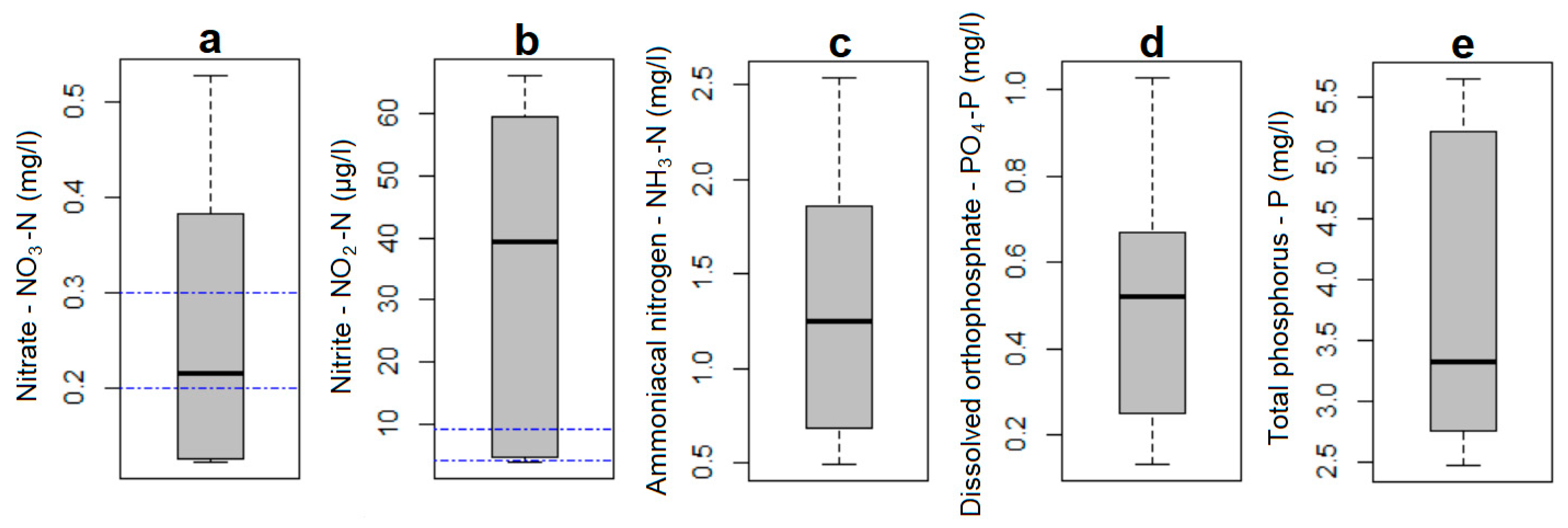
Figure 4 shows the results of the measurements of the parameters, nitrates NO₃-N, nitrites NO₂-N, ammoniacal nitrogen (NH₃-N), dissolved orthophosphate PO₄-P and total phosphorus (P), which were carried out during the last two CSO events in the El Vado (Table A2). The samplings registered values for nitrate between 0.12 to 0.53 mg/L (Figure 4a). Jerves-Cobo et al. [24] determined NO₃-N values between 0.2 to 0.3 mg/L for the stretch of river between the three CSOs during the wet season. The nitrite concentration in the El Vado CSO was in the order of 3.74 to 66.27 μg/L (Figure 4b). According to Jerves-Cobo et al. [24], the NO₂-N values measured in the corresponding section of the Tomebamba River varied between 3.3 and 8.2 μg/L in the rainy season. Based on the parameters NO₃-N and NO₂-N, it is evident that the El Vado CSO contributes to the deterioration of the waters of the Tomebamba River during CSO events. The dissolved orthophosphate values were in the range of 0.13 to 1.03 mg/L, with a mean value of 0.49 mg/L (Figure 4d). Ammoniacal nitrogen ranged from 0.49 to 2.54 mg/L, with a mean value of 1.34 mg/L (Figure 4c). Finally, the total phosphorus values were between 2.47 to 5.65 mg/L, with an average value of 3.77 mg/L (Figure 4e). Ecuadorian regulations establish a maximum daily mean value of 30 mg/L for ammoniacal nitrogen and 10 mg/L for total phosphorus [26], for the discharge of effluents into a body of fresh water. The concentrations of these two parameters in CSO El Vado are below their respective limits.

BOD₅/COD Ratio

One of the most important characteristics of wastewater is its biodegradability, which informs the feasibility of applying biologic treatment methods. The relationship between the five-day biochemical oxygen demand and chemical oxygen demand (BOD₅/COD) for all the samples analyzed was in the range of 0.04 to 0.92. This result evidences a high variation in the carbon sources of wastewater, showing a wide range from small to large amounts of biodegradable matter in wastewaters [22].

Table 2. The BOD₅/COD ratio for the samples recorded throughout the study period of March 2017 to May 2018.

CSO	BOD5/COD			Standard Deviation
	Max	Min	Mean
El Vado	0.81	0.04	0.38	0.24
Multifamiliares	0.92	0.17	0.52	0.33
Coliseo	0.63	0.34	0.44	0.16

shows that the Multifamiliares and El Vado CSOs display a greater range of variability, presenting a larger range in the type of pollutants.

Jerves-Cobo et al. [22] adjusted the relationship between the BOD₅ and COD variables by means of a logarithmic regression with an R² of 0.62. In this study, it was determined that the data fit better with a quadratic relationship, in which R² was 0.73 (Appendix A—Figure A1). These results can be used for the prediction of in discharges from the values.

3.2. Environmental Legislation

Ecuadorian legislation establishes water quality criteria for the discharge of effluents into freshwater bodies [26]. This regulation only limits the concentrations of the daily mean values of the effluents. For the average values of COD in the Multifamiliares discharge, 67% of the events were below the concentrations established in the regulations (COD ≤ 200 mg/L). In the El Vado CSO, 33% of the events complied with the regulations. This CSO is an important source of contamination since it provides a greater volume of flow compared to other discharges. The Coliseo CSO presents high COD values, showing that none of the registered events complied with the environmental regulations for the discharge of effluents in freshwater receiving bodies.

For BOD₅, only one sample was analyzed for each CSO event. Therefore, it was not possible to establish a characteristic mean value for the discharge event. However, for the purposes of comparison with the regulations, it is assumed that the point value obtained represents the average concentration of the CSO event. Thus, in the discharge data for Multifamiliares, 67% of the samples comply with the limits established by the legislation for the parameter For BOD₅ (≤100 mg/L). In the El Vado CSO, 56% of the samples comply with the regulations and in the Coliseo CSO, none of the samples meet the limits of BOD₅. For the microbiological parameters, the regulations establish a limit of 2000 MPN/100 mL for the daily average value of fecal coliforms [26]. Although the mean total coliform values were not obtained for each CSO event, all the samples analyzed recorded values above this limit (between 800 and 1.0 × 10⁷ times higher).

The results show the need for legislation that incorporates specific parameters that characterize the combined sewer overflow processes, an aspect that has already been implemented in other places around the world [13]. For instance, in the province of Quebec, Canada, the legislation recommends a maximum frequency of seven CSO spill per year under wet weather conditions [27].

3.3. Dynamics of Pollutants during CSO

Figure 5, Figure A2 and Figure A3 show the results of the variation of conductivity, turbidity and COD parameters in the events selected under criteria (i) and (ii) (described in Section 2.4) in the El Vado, Multifamiliares and Coliseo CSOs.

In the El Vado (Figure 5) and Coliseo (Figure A3) CSOs, despite the peak flow being higher in event i, the average values of conductivity, turbidity and COD are higher in event ii. However, in the Multifamiliares CSO (Figure A2), event ii (which has the highest flow) coincides with the highest records of concentrations of conductivity, turbidity and COD. This analysis suggests that the concentration values of these pollutants do not necessarily grow with the magnitude of the CSO event in terms of flow.

Some characteristics of the pollutants observed in the six analyzed events were identified, regardless of the discharge or the application of criterion i or ii. These characteristics are analyzed below.

Figure 5a(i,ii), Figure A2a(i,ii) and Figure A3a(i,ii) show that peak conductivity values occur between the initial part of the CSO event and the maximum flow value of the discharge hydrograph in the three CSOs. This suggests a higher degree of contamination related to dissolved pollutants at the start of the CSO event. A similar conclusion was reached by Passerat et al. [2], who evaluated the variation in the contaminating components during a precipitation event in one of the main CSOs that discharge to the Seine River in Paris, France.

In all the events analyzed and presented in Figure 5b(i,ii), Figure A2b(i,ii) and Figure A3b(i,ii), the maximum turbidity values occur near the discharge peak flow of the discharge hydrograph; a similar result was determined by García et al. [56]. Turbidity is related to the suspended matter load in the wastewater. The increase in turbidity in the maximum section of the hydrograph may be due to the resuspension of sedimented material in the pipes, caused by an increase in tractive force due to an increase in flow. Passerat et al. [2] determined that around 75% of the suspended matter found in the combined sewer discharge came from the resuspension of sedimented particles in the pipes. The authors also determined that the intensity of precipitation influences the percentage of suspended matter found in the wastewater during discharge.

3.4. Relationship between Rain and the CSO Characteristics

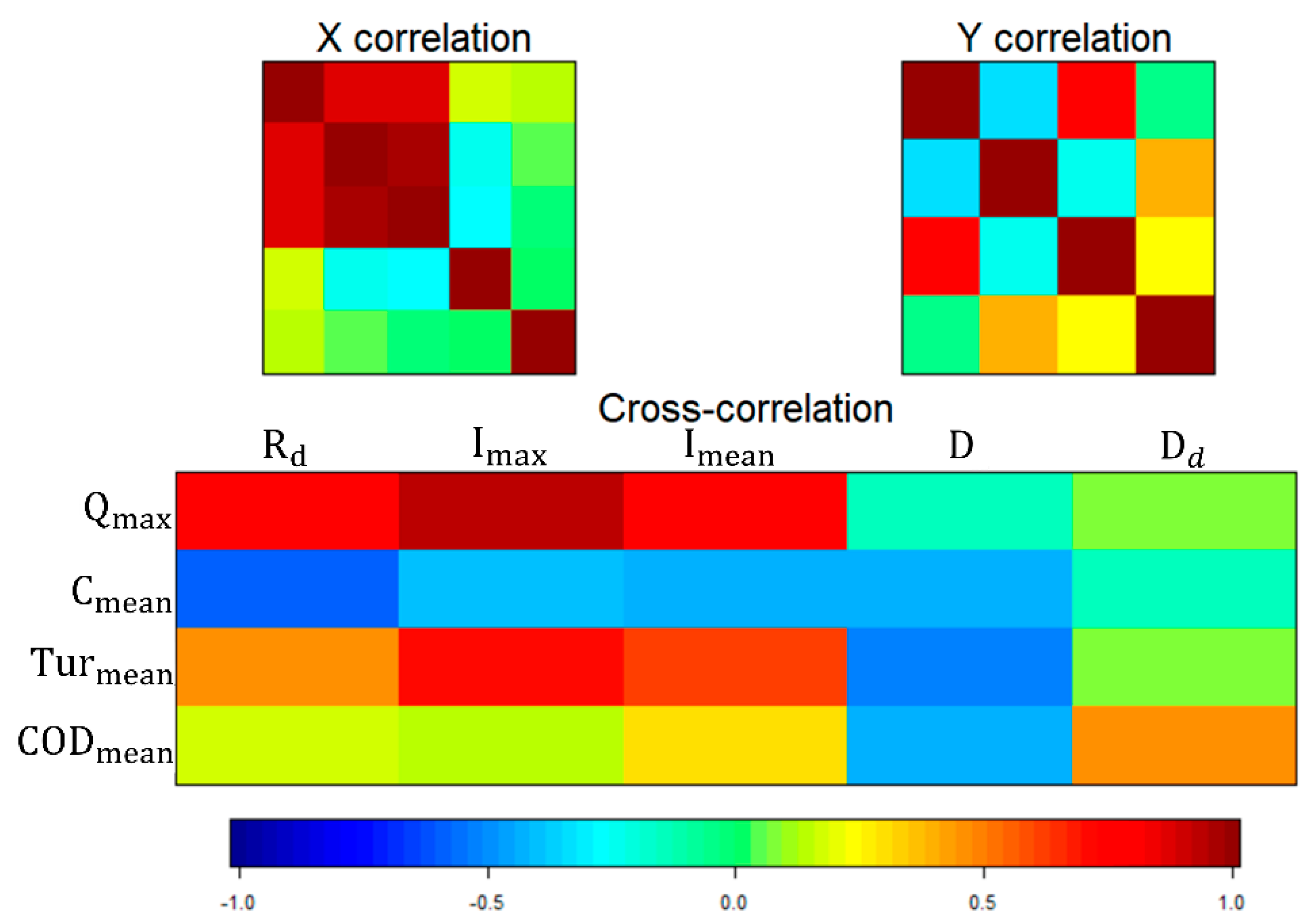
Correlation matrices that are complementary to the CCA were preliminarily analyzed [36,38,43]. These results allow one to visualize the relationship between rainfall and CSO variables for the three CSOs (Figure 6, Figure A4 and Figure A5).

The correlation graph for the El Vado (Figure 6) and Multifamiliares (Figure A4) CSOs shows that the average intensity of rain (I_mean), has an influence on the maximum discharge flow (Q_max), for this correlations a p value less than 0.05 was obtained (

Table A3. Statistical significance (p values) of the correlations between the variables of rainfall and CSO in the El Vado CSO.

	${\mathbf{R}}_{\mathbf{d}}$	${\mathbf{I}}_{\mathbf{max}}$	${\mathbf{I}}_{\mathbf{mean}}$	$\mathbf{D}$	${\mathbf{D}}_{\mathbf{d}}$
${\mathrm{Q}}_{\max }$	0.01	${7.0\times 10}^{-4}$	0.02	0.75	0.85
${\mathrm{C}}_{\mathrm{mean}}$	0.18	0.39	0.33	0.35	0.74
${\mathrm{Tur}}_{\mathrm{mean}}$	0.22	0.04	0.08	0.16	0.84
${\mathrm{COD}}_{\mathrm{mean}}$	0.65	0.72	0.46	0.26	0.23

and

Table A4. Statistical significance (p values) of the correlations between the variables of rainfall and CSO in the Multifamiliares CSO.

	${\mathbf{R}}_{\mathbf{d}}$	${\mathbf{I}}_{\mathbf{max}}$	${\mathbf{I}}_{\mathbf{mean}}$	$\mathbf{D}$	${\mathbf{D}}_{\mathbf{d}}$
${\mathrm{Q}}_{\max }$	0.60	0.10	0.04	0.51	0.89
${\mathrm{C}}_{\mathrm{mean}}$	0.34	0.63	0.56	0.68	0.14
${\mathrm{Tur}}_{\mathrm{mean}}$	0.91	0.25	0.04	0.33	0.01
${\mathrm{COD}}_{\mathrm{mean}}$	0.96	0.48	0.12	0.44	0.36

). It is considered a significant correlation. Furthermore, in the El Vado CSO the maximum intensity of precipitation (I_max) is related to the maximum flow Q_max (p value < 0.05). This same relationship is obtained in the Multifamiliares CSO, but with p value of 0.10. Sandoval et al. [14], in their research on the main CSO in Berlin, found that the maximum and average intensity of precipitation is related to the volume of water discharged, as well as the maximum flow and the average discharge flow. At CSO El Vado, a significant relationship was also found between total precipitation R_d and maximum flow Q_max.

In the El Vado and Multifamiliares CSOs, the I_max and I_mean respectively also seem to influence the values of the average turbidity (Tur_mean) (Figure 6 and Figure A4). In the same way, these correlations obtained a p value less than 0.05. According to Murillo [57], turbidity helps determine the amount of suspended material, where the higher the intensity of rain is, the greater the drag of suspended solids will be. Likewise, Sandoval et al. [14] found a relationship between I_max and I_mean with the value of total suspended solids.

For the Multifamiliares CSO (Figure A4), it was also found that the Tur_mean is related to the duration of the dry period prior to a rainfall event (D_d) with a statistical significance related to a p value less than 0.05. In this CSO, it was also found that the COD_mean is related to the average intensity of precipitation (I_mean) with a p value of 0.12. D_d and I_mean, which can influence the amount of drag material due to the runoff and resuspension of material deposited in the drainage ducts that cause higher pollution loads [2,14,20].

The results of the correlational analysis between the rainfall and CSO parameters for the Multifamiliares CSO showed a similar pattern to the results obtained for the El Vado CSO, mainly between the parameters I_max, I_mean, Q_max and Tur_mean.

When comparing the correlation graphs of the three CSOs (Figure 6, Figure A4 and Figure A5), it can be seen that the correlation matrix of the Coliseo CSO is very different from the other two. This discrepancy could be due to the Coliseo CSO registering only three trials, unlike the other two CSOs, for which more trials were performed. For this, it is recommended in a future study to take a similar quantity sample in each CSO to obtain comparable results. For this reason, given the small sample size, the results for the Coliseo CSO should be interpreted with caution.

3.4.1. Canonical Correlation Analysis

The Canonical Correlation Analysis was carried out only for the El Vado CSO. For the Multifamiliares and Coliseo, it was not possible to perform a CCA due to the insufficient number of available trials (six trials or less) [43].

From the CCA, only two canonical variables L(1) and L(3) were found to be statistically significant (p value ≈ 0). For both canonical variables, the correlation is close to one. This means that two canonical correlations would be sufficient to measure the association between the rainfall and CSO variables [41].

Table 3. Canonical loads (ρ) between (a) the explanatory rain variables and (b) response variables, with the significant canonical variables L(1) and L(3) for the El Vado CSO. Values that represent the possible influence of rainfall variables on CSO are highlighted in gray.

(a)			(b)
	L(1)	L(3)		L(1)	L(3)
Rd	0.582	−0.573	Qmax	0.992	0.03
Imax	0.948	3 × 10−4	Cmean	−0.441	0.252
Imean	0.626	0.219	Turmean	0.809	0.503
D	0.026	−0.832	CODmean	−0.238	0.123
Dd	0.263	−0.392

a shows the canonical loadings (ρ) obtained between L(1) and L(3) and the rainfall characteristics (independent variables). On the other hand, Table 3b shows the canonical loadings obtained between the canonical variables L(1) and L(3) and the characteristics of the CSO (response variables).

Regarding the CCA presented for the El Vado CSO, in Table 3a,b, the values of ρ greater than 0.4–0.5 between L(1) and L(3) and the characteristics of rainfall and CSO indicate the possible influence of rainfall on the CSO variables, an aspect consistent with the results found by Sandoval et al. [14]. From the analysis of L(1), the maximum intensity of rainfall (I_max), the average intensity (I_mean) and the total rainfall depth (R_d) seem to have influence on the variables Q_max and Tur_mean. These relationships agree with those obtained from the analysis of the correlation matrices. From the analysis of L(3), it was determined that the duration of the rain (D) and the total rainfall depth (R_d) (to a lesser degree) are related to the mean turbidity values (Tur_mean).

3.4.2. Partial Least Squares Regression (PLSR)

Next, we describe the construction of the PLSR model for the pollutant Tur_mean at the El Vado CSO. In the same way, the PLSR prediction models were determined for the other dependent variables, C_mean, COD_mean, and Q_max, for all CSOs.

Figure A6 shows the root mean squared error of Prediction (RMSEP) for the variable Tur_mean as a function of the number of components used in the construction of the model.

Table 4. Percentages of variance explained according to the number of components of the PLS model for prediction of the variable Tur_mean in the El Vado CSO.

	1 Comp	2 Comp	3 Comp	4 Comp	5 Comp
Explained variance (%)	77.17	92.23	99.06	99.98	100

shows the percentage of variability explained by each of the components of the model. Considering the reduction of the RMSEP and the levels of variability explained, two components were determined for the construction of the PLS model to predict Tur_mean for the El Vado CSO (Figure A7).

After performing the PLSR for all the dependent variables, fit equations were obtained that can estimate the output CSO characteristics (COD_mean, C_mean, Tur_mean, Q_max) based on the input rainfall characteristics (R_d, I_max, I_mean, D and D_d). The structure of the PLSR is reported in Equation (1).

$$\mathrm{CSO}=\mathrm{C}1\times {\mathrm{R}}_{\mathrm{d}}+{\mathrm{C}}_2\times {\mathrm{I}}_{\max }+{\mathrm{C}}_3\times {\mathrm{I}}_{\mathrm{mean}}+{\mathrm{C}}_4\times \mathrm{D}+{\mathrm{C}}_5\times {\mathrm{D}}_{\mathrm{d}}+{\mathrm{C}}_6$$

(1)

the regression coefficients (C₁, C₂, C₃, C₄, C₅ and C₆) of the PLSR models for the prediction of the CSO variables in the El Vado CSO are presented in

Table 5. Regression coefficients for the prediction equations of the CSO variables as a function of the rainfall parameters for the El Vado CSO. R² is the coefficient of determination of the PLSR.-N is the number of components used to build the PLSR model, and X is the percentage of variability explained by the model.

CSO Variable	Regression Coefficients (PLSR)						N	X (%)	R2
	${\mathbf{C}}_{\mathbf{1}}$	${\mathbf{C}}_{\mathbf{2}}$	${\mathbf{C}}_{\mathbf{3}}$	${\mathbf{C}}_{\mathbf{4}}$	${\mathbf{C}}_{\mathbf{5}}$	${\mathbf{C}}_{\mathbf{6}}$
${\mathrm{Q}}_{\max }$	7.710	33.740	9.892	1.217	2.300	−29.932	2	92.2	0.81
${\mathrm{C}}_{\mathrm{mean}}$	−8.428	−0.584	−26.091	−0.989	2.079	373.142	4	98.0	0.62
${\mathrm{Tur}}_{\mathrm{mean}}$	0.404	1.792	0.513	−0.516	0.207	170.928	2	92.2	0.60
${\mathrm{COD}}_{\mathrm{mean}}$	16.281	−11.664	23.326	−1.399	3.480	279.929	4	99.7	0.71

. The results of the PLSR for the Multifamiliares and Coliseo CSOs are presented in

Table A5. Regression coefficients for the prediction equations of the CSO variables as a function of the rainfall parameters for the Multifamiliares CSO. R² is the coefficient of determination of the PLSR.-N is the number of components used to build the PLSR model and X is the percentage of variability explained by the model.

CSO Variable	Regression Coefficients (PLSR)						N	X (%)	R2
	${\mathbf{C}}_{\mathbf{1}}$	${\mathbf{C}}_{\mathbf{2}}$	${\mathbf{C}}_{\mathbf{3}}$	${\mathbf{C}}_{\mathbf{4}}$	${\mathbf{C}}_{\mathbf{5}}$	${\mathbf{C}}_{\mathbf{6}}$
${\mathrm{Q}}_{\max }$	3.638	20.553	2.152	−1.919	−9.809	314.896	2	96.1	0.57
${\mathrm{C}}_{\mathrm{mean}}$	−0.394	−1.568	−0.653	0.017	4.311	138.720	2	97.5	0.57
${\mathrm{Tur}}_{\mathrm{mean}}$	0.965	4.469	1.745	−0.423	6.720	26.148	2	99.0	0.91
${\mathrm{COD}}_{\mathrm{mean}}$	1.898	10.873	9.220	−0.834	8.214	44.239	3	99.9	0.37

and

Table A6. Regression coefficients for the prediction equations of the CSO variables as a function of the rainfall parameters for the Coliseo CSO. R₂ is the coefficient of determination of the PLSR.-N is the number of components used to build the PLSR model and X is the percentage of variability explained by the model.

CSO Variable	Regression Coefficients (PLSR)						N	X (%)	R2
	${\mathbf{C}}_{\mathbf{1}}$	${\mathbf{C}}_{\mathbf{2}}$	${\mathbf{C}}_{\mathbf{3}}$	${\mathbf{C}}_{\mathbf{4}}$	${\mathbf{C}}_{\mathbf{5}}$	${\mathbf{C}}_{\mathbf{6}}$
${\mathrm{Q}}_{\max }$	0.592	1.093	−0.058	5.594	4.266	−95.744	1	96.6	0.84
${\mathrm{C}}_{\mathrm{mean}}$	−0.114	−0.167	0.025	−1.114	−0.768	256.847	1	96.6	0.65
${\mathrm{Tur}}_{\mathrm{mean}}$	−0.199	−0.331	0.031	−1.909	−1.389	345.263	1	96.6	0.75
${\mathrm{COD}}_{\mathrm{mean}}$	−0.240	0.217	0.230	−2.835	−0.924	586.029	1	95.7	0.18

, respectively.

The determination coefficient ${\mathrm{R}}^2$ for the prediction of the CSO parameters in the El Vado CSO ranged from 0.60 to 0.81 (Table 5); for the Multifamiliares CSO, this value was between 0.91 and 0.37 (Table A5) and for the Coliseo CSO, it was in the range of 0.84 and 0.18 (Table A6). On average, the El Vado CSO presents the highest values of ${\mathrm{R}}^2$, this means that in this CSO, the equations had a better fit.

The lowest ${\mathrm{R}}^2$ values were recorded in the determination of ${\mathrm{COD}}_{\mathrm{mean}}$ for the Multifamiliares and Coliseo CSOs (0.37 and 0.18, respectively). These last CSOs have a contribution area approximately three times smaller than the El Vado CSO area. On the other hand, the ${\mathrm{R}}^2$ value obtained for the prediction of ${\mathrm{COD}}_{\mathrm{mean}}$ in the El Vado CSO was 0.71 (Table 5). This result suggests that the equations obtained for the ${\mathrm{COD}}_{\mathrm{mean}}$ would be better fitted to a larger basin.

In the Coliseo CSO, the values of ${\mathrm{R}}^2$ showed the widest range of variability. This may be because a smaller number of tests were performed on this combined sewer overflow compared to the other two CSOs, which may have affected the fit of the prediction equations. Thus, in the El Vado CSO nine CSO events were registered with a total of 161 samples, while in the Multifamiliares CSO six events were registered with 124 samples, finally in the Coliseo CSO three CSO events were registered with 46 samples (Table A2).

The average of the ${\mathrm{R}}^2$ values for the prediction of the variables ${\mathrm{C}}_{\mathrm{mean}}$ and ${\mathrm{Q}}_{\max }$ in the three CSOs presents a smaller range of variation than in the other two variables. This suggests that the ${\mathrm{C}}_{\mathrm{mean}}$ and ${\mathrm{Q}}_{\max }$ possibly contain less uncertainty or that their predictions are less sensitive to the uncertainty of the rain. Sandoval et al. [14] found a similar result for these same variables.

For the prediction of ${\mathrm{COD}}_{\mathrm{mean}}$ in the Coliseo CSO, a low determination coefficient (${\mathrm{R}}^2=0.18$) was obtained. The value of ${\mathrm{R}}^2$ measures the goodness of fit-of-the-model to a set of data [58], in this case, the equation obtained for ${\mathrm{COD}}_{\mathrm{mean}}$ in the Coliseo CSO does not have a good fit, so it is considered a low precision model.

The PLSR results are also displayed through a triplot that represents the cases, the response variables (CSO: ${\mathrm{Q}}_{\max }$, ${\mathrm{C}}_{\mathrm{mean}}$, ${\mathrm{Tur}}_{\mathrm{mean}}$, ${\mathrm{COD}}_{\mathrm{mean}}$) and the predictor variables (Rainfall: ${\mathrm{R}}_{\mathrm{d}}$, ${\mathrm{I}}_{\max }$, ${\mathrm{I}}_{\mathrm{mean}}$, $\mathrm{D}$, ${\mathrm{D}}_{\mathrm{d}}$) measures for the same cases. Figure 7 shows the triplot for the El Vado CSO, while the triplots for the Multifamiliares and Coliseo CSOs are shown in Figure A8 and Figure A9, respectively.

The triplots of the El Vado and Multifamiliares CSO (Figure 7 and Figure A8, respectively) showed similar relationships between the variables of rainfall and CSO. These results are consistent with the relationships that were determined through the correlation analysis and CCA. In these two CSOs, a correlation was determined between the independent variables ${\mathrm{I}}_{\max }$ and ${\mathrm{R}}_{\mathrm{d}}$ with dependent variable ${\mathrm{Q}}_{\max }$. A relationship of the average intensity (${\mathrm{I}}_{\mathrm{mean}}$) with the average Turbidity (${\mathrm{Tur}}_{\mathrm{mean}}$) was also observed, as well as a positive relationship between ${\mathrm{D}}_{\mathrm{d}}$ and the ${\mathrm{COD}}_{\mathrm{mean}}$. Similarly, a negative relationship between the total rainfall depth (${\mathrm{R}}_{\mathrm{d}}$) and mean conductivity (${\mathrm{C}}_{\mathrm{mean}}$) was observed.

The triplot obtained for the Coliseo CSO (Figure A9) differs from the triplots made for the El Vado (Figure 7) and Multifamiliares (Figure A8) CSOs. As mentioned above, this may be due to the small sample size used in the Coliseo CSO analysis.

The relationships found determine the influence of rainfall parameters on the behavior and dynamics of pollutants during CSO events. These relationships can be used in the construction of integrated ecological models for the evaluation and complete analysis of the city’s sanitation systems, their impact on the receiving bodies and their restoration.

4. Conclusions

The El Vado, Multifamiliares and Coliseo CSOs contribute to the deterioration of the water quality of the Tomebamba River during the rainy season. There was a high variation in the type of wastewater related to the content of biodegradable material in the CSOs. There was also great temporal variability in the water quality parameters during CSO events. For conductivity, in the three CSOs, the highest values were presented between the beginning of the CSO event and the maximum discharge value obtained in the hydrograph. On the other hand, the maximum turbidity values were located relatively close to the peak flow of the discharge hydrograph.

From the analysis of the relationship between rainfall and CSO characteristics carried out with the CCA and PLSR methods, it is concluded that (i) The maximum discharge flow of a CSO is mainly related to the maximum intensity of rainfall and, to a lesser degree, the average intensity and total rainfall depth; (ii) The average rainfall intensity and, the maximum intensity, both influence the average turbidity values; (iii) The average turbidity is positively related to the duration of the dry season prior to a precipitation event and to the average intensity of rainfall. (iv) The mean turbidity is also negatively related to the duration of a precipitation event. (v) The total rainfall depth showed a negative relationship with average conductivity.

References

1. Morgan, D.; Xiao, L.; McNabola, A. Evaluation of combined sewer overflow assessment methods: Case study of Cork City, Ireland. Water Environ. J. 2017, 65, 202–208. [Google Scholar] [CrossRef]
2. Passerat, J.; Ouattara, N.K.; Mouchel, J.-M.; Rocher, V.; Servais, P. Impact of an intense combined sewer overflow event on the microbiological water quality of the Seine River. Water Res. 2011, 45, 893–903. [Google Scholar] [CrossRef] [PubMed]
3. Yü, Y.; Kojima, K.; An, A.K.; Furumai, H. Cluster analysis for characterization of rainfalls and CSO behaviours in an urban drainage area of Tokyo. Water Sci. Technol. 2013, 68, 544–551. [Google Scholar] [CrossRef] [PubMed]
4. Brokamp, C.; Beck, A.F.; Muglia, L.; Ryan, P. Combined sewer overflow events and childhood emergency department visits: A case-crossover study. Sci. Total. Environ. 2017, 607, 1180–1187. [Google Scholar] [CrossRef]
5. Al Aukidy, M.; Verlicchi, P. Contributions of combined sewer overflows and treated effluents to the bacterial load released into a coastal area. Sci. Total. Environ. 2017, 483–496. [Google Scholar] [CrossRef]
6. Hvitved-Jacobsen, T. The impact of combined sewer overflows on the dissolved oxygen concentration of a river. Water Res. 1982, 16, 1099–1105. [Google Scholar] [CrossRef]
7. Madoux-Humery, A.-S.; Dorner, S.; Sauvé, S.; Aboulfadl, K.; Galarneau, M.; Servais, P.; Prévost, M. The effects of combined sewer overflow events on riverine sources of drinking water. Water Res. 2016, 92, 218–227. [Google Scholar] [CrossRef]
8. Weyrauch, P.; Matzinger, A.; Pawlowsky-Reusing, E.; Plume, S.; Von Seggern, D.; Heinzmann, B.; Schroeder, K.; Rouault, P. Contribution of combined sewer overflows to trace contaminant loads in urban streams. Water Res. 2010, 44, 4451–4462. [Google Scholar] [CrossRef]
9. Mulliss, R.; Revitt, D.; Shutes, R. The impacts of discharges from two combined sewer overflows on the water quality of an urban watercourse. Water Sci. Technol. 1997, 36, 195–199. [Google Scholar] [CrossRef]
10. Valdez, C.; Vásquez, A. Ingeniería de los Sistemas de Tratamiento y Disposición Deaguas Residuales; Fundación Ica: México D.F., México, 2003; p. 341. [Google Scholar]
11. Tchobanoglous, G.; Burton, F.L.; Eddy, M. Ingeniería de Aguas Residuales: Tratamiento, Vertido y Reutilización; McGraw-Hill: Madrid, España, 1995; ISBN 9788448116071. [Google Scholar]
12. Gómez, E.G. Combinar o separar? Una discusión con un siglo de antigüedad y de gran actualidad para los bogotanos. Rev. Ing. 2000, 11, 21–30. [Google Scholar]
13. Mailhot, A.; Talbot, G.; Lavallée, B. Relationships between rainfall and combined sewer overflow (CSO) occurrences. J. Hydrol. 2015, 523, 602–609. [Google Scholar] [CrossRef]
14. Sandoval, S.; Torres, A.; Pawlowsky-Reusing, E.; Riechel, M.; Caradot, N. The evaluation of rainfall influence on combined sewer overflows characteristics: The Berlin case study. Water Sci. Technol. 2013, 68, 2683–2690. [Google Scholar] [CrossRef] [PubMed]
15. Kreutzberger, W.A.; Race, R.A.; Meinholz, T.L.; Harper, M.; Ibach, J. Impact of sediments on dissolved oxygen concentrations following combined sewer overflows. J. Water Pollut. Control Fed. 1980, 52, 192–201. [Google Scholar]
16. Brzezińska, A.; Zawilski, M.; Sakson, G. Assessment of pollutant load emission from combined sewer overflows based on the online monitoring. Environ. Monit. Assess. 2016, 188, 1–10. [Google Scholar] [CrossRef] [Green Version]
17. Riechel, M.; Matzinger, A.; Pawlowsky-Reusing, E.; Sonnenberg, H.; Uldack, M.; Heinzmann, B.; Caradot, N.; Von Seggern, D.; Rouault, P. Impacts of combined sewer overflows on a large urban river—Understanding the effect of different management strategies. Water Res. 2016, 105, 264–273. [Google Scholar] [CrossRef]
18. Suárez, J.; Puertas, J. Determination of COD, BOD, and suspended solids loads during combined sewer overflow (CSO) events in some combined catchments in Spain. Ecol. Eng. 2005, 24, 199–217. [Google Scholar] [CrossRef]
19. Ruan, M. Continuous simulation of CSO emissions. Urban Water 1999, 1, 201–205. [Google Scholar] [CrossRef]
20. Bi, E.G.; Monette, F.; Gasperi, J. Analysis of the influence of rainfall variables on urban effluents concentrations and fluxes in wet weather. J. Hydrol. 2015, 523, 320–332. [Google Scholar] [CrossRef]
21. ETAPA-EP. Evolución de la Calidad del Agua en los Ríos que Atraviesan la Ciudad de Cuenca; ETAPA-EP, Dirección de manejo Ambiental: Cuenca, Ecuador, 2007. [Google Scholar]
22. Jerves-Cobo, R.; Benedetti, L.; Amerlinck, Y.; Lock, K.; De Mulder, C.; Van Butsel, J.; Cisneros, F.; Goethals, P.; Nopens, I. Integrated ecological modelling for evidence-based determination of water management interventions in urbanized river basins: Case study in the Cuenca River basin (Ecuador). Sci. Total. Environ. 2020, 709, 136067. [Google Scholar] [CrossRef]
23. Jerves-Cobo, R.; Forio, M.A.E.; Lock, K.; Van Butsel, J.; Pauta, G.; Cisneros, F.; Nopens, I.; Goethals, P.L. Biological water quality in tropical rivers during dry and rainy seasons: A model-based analysis. Ecol. Indic. 2020, 108, 105769. [Google Scholar] [CrossRef]
24. Jerves-Cobo, R.; Lock, K.; Van Butsel, J.; Pauta, G.; Cisneros, F.; Nopens, I.; Goethals, P.L.M. Biological impact assessment of sewage outfalls in the urbanized area of the Cuenca River basin (Ecuador) in two different seasons. Limnologica 2018, 71, 8–28. [Google Scholar] [CrossRef]
25. Temprano-Gonzales, J.; Gabriel-Cervigni, M.; Suárez-Lopez, J.; Tejero-Monzón, J. Contaminación en redes de alcantarillado urbano en tiempo de lluvia: Control de origen. Rev. Obras Públicas 1996, 143, 45–57. [Google Scholar]
26. MAE. Texto Unificado Legislacion Secundaria de Medio Ambiente; Lexis: Quito, Ecuador, 2017; ISBN 9788578110796. [Google Scholar]
27. Jean, M.È.; Duchesne, S.; Pelletier, G.; Pleau, M. Selection of rainfall information as input data for the design of combined sewer overflow solutions. J. Hydrol. 2018, 565, 559–569. [Google Scholar] [CrossRef]
28. Jerves-Cobo, R.; Córdova-Vela, G.; Goethals, P.L.M.; Díaz-Granda, C.; Van Echelpoel, W.; Cisneros, F.; Nopens, I.; Goethals, P.L.M. Model-based analysis of the potential of macroinvertebrates as indicators for microbial pathogens in rivers. Water 2018, 10, 375. [Google Scholar] [CrossRef] [Green Version]
29. Jerves-Cobo, R.; Everaert, G.; Goethals, P.L.M.; Córdova-Vela, G.; Díaz-Granda, C.; Cisneros, F.; Nopens, I.; Goethals, P.L.M. A methodology to model environmental preferences of EPT taxa in the Machangara river basin (Ecuador). Water 2017, 9, 195. [Google Scholar] [CrossRef] [Green Version]
30. Aereopuerto-Mariscal-Lamar. Información Meteorológica Aereopuerto Mariscal Lamar Cuenca; Dirección de aviación civil del Ecuador: Quito, Ecuador, 2012. [Google Scholar]
31. INEC. Proyección de la Población Ecuatoriana, por Años Calendario, Según Cantones 2010–2020. Available online: https://www.ecuadorencifras.gob.ec/proyecciones-poblacionales/ (accessed on 16 December 2019).
32. Arévalo, M.; Van Echelpoel, W.; Alvarado, A.; Goethals, P.; Larriva, J. Análisis espacial-temporal de procesos relacionados con concentraciones de oxígeno disuelto en lagunas de maduración. MASKANA 2017, 8, 115–123. [Google Scholar] [CrossRef] [Green Version]
33. Alvarado, A.; Vedantam, S.; Durazno, G.; Nopens, I. Hydraulic assessment of waste stabilization ponds: Comparison of computational fluid dynamics simulations against tracer data. MASKANA 2011, 2, 81–89. [Google Scholar] [CrossRef]
34. Aparicio Mijares, F.J. Fundamentos de Hidrología de Superficie; 8. reimpr.; Limusa Noriega: México D.F., México, 1999; ISBN 968-18-3014-8. [Google Scholar]
35. Leurgans, S.E.; Moyeed, R.A.; Silverman, B.W. Canonical correlation analysis when the data are curves. J. R. Stat. Soc. Ser. B Statistical Methodol. 1993, 55, 725–740. [Google Scholar] [CrossRef]
36. De Leeuw, J. Journal of Statistical Software. Wiley Interdiscip. Rev. Comput. Stat. 2009, 1, 128–129. [Google Scholar] [CrossRef] [Green Version]
37. Yu, Y.; Zhang, S.; An, A.K.; Furumai, H. Simple method for calculating hydraulic behavior of combined sewer overflow from rainfall event data. J. Water Resour. Plan. Manag. 2018, 144, 04018061. [Google Scholar] [CrossRef]
38. Valentukevičienė, M.; Bagdžiūnaitė-Litvinaitienė, L.; Chadyšas, V.; Litvinaitis, A. Evaluating the impacts of integrated pollution on water quality of the trans-boundary Neris (Viliya) River. Sustainability 2018, 10, 4239. [Google Scholar] [CrossRef] [Green Version]
39. R-Core-Team R. A Language and Environment for Statistical Computing; R Foundation for Statistical Computing: Vienna, Austria, 2017. [Google Scholar]
40. InfoStat-Team. InfoStat Software Estadístico; Grupo Infostat: Córdova, Argentina, 2019. [Google Scholar]
41. Balzarini, M.; Córdoba, M.; Bruno, C.; Teich, I. Herramientas en el Análisis Estadístico Multivariado; Escuela Virtual CAVILA: Córdova, Argentina, 2015. [Google Scholar]
42. Cuadras, C.M. Nuevos metodos de analisis multivariante. Rev. Española Quimioter. Publicación Soc. Española Quimioter. 2007, 20, 249. [Google Scholar]
43. Badii, M.; Castillo, J.; Cortez, K.; Wong, A.; Villalpando, P. Análisis Correlación Canónica (ACC) investigación científica. Investig. Sci. 2007, 4, 405–422. [Google Scholar]
44. Mevik, B.-H.; Wehrens, R. TheplsPackage: Principal component and partial least squares regression in R. J. Stat. Softw. 2007, 18, 1–23. [Google Scholar] [CrossRef] [Green Version]
45. Gregoria, M.; Aparicio, M.; Antonio, C. La regresión por mínimos cuadrados parciales. Orígenes y Evolución. In Historia de la probabilidad y la estadística (IV); Universidad de Huelva: Sevilla, España, 2009; pp. 441–448. [Google Scholar]
46. Vilca, J.C.V.; Guzman, J. Regresion PLS y PCA como solución al problema de multicolinealidad en regresion multiple. Rev. Matemática Teoría Apl. 2011, 18, 9–20. [Google Scholar] [CrossRef] [Green Version]
47. Gaviria, C. Regresión por Mínimos Cuadrados Parciales PLS Aplicada a Datos Variedad Valuados; Universidad Nacional de Colombia: Medellín, Colombia, 2015; pp. 18–21. [Google Scholar]
48. Wold, H. Model Construction and Evaluation when Theoretical Knowledge Is Scarce: Theory and Application of Partial Least Squares; Academic Press: Uppsala, Sweden, 1980; pp. 47–74. [Google Scholar]
49. Bellosta, C.J.G. R Para Profesionales de los Datos: Una Introducción. 2018, p. 139. Available online: https://www.datanalytics.com/libro_r/ (accessed on 26 July 2020).
50. Falk, R.F.; Miller, N.B. A Primer for Soft Modelling; The University of Akron: Akron, OH, USA, 1992. [Google Scholar]
51. Abdi, H. Partial least squares (PLS) regression. In Encyclopedia of Social Sciences Research Methods; Lweis-Beck, A.M., Bryman, T., Eds.; Sage: Thousand Oaks, CA, USA, 2003; pp. 792–795. [Google Scholar]
52. Bertrand, D. Etalonnage Multidimensionnel: Application aux Données Spectrales (Multi-dimensional calibration: Application to Spectral Data; Techniques de I’ngénieur: Paris, France, 2005. [Google Scholar]
53. Martínez Galera, M.; Martínez Vidal, J.L.; Garrido Frenich, A.; Gil García, M.D. Evaluation of multi-wavelength chromatograms for the quantification of mixtures of pesticides by high-performance liquid chromatography-diode array detection with multivariate calibration. J. Chromatogr. 1997, 778, 139–149. [Google Scholar] [CrossRef]
54. Hintze, J.L.; Nelson, R.D. Violin plots: A box plot-density trace synergism. Am. Stat. 1998, 52, 181–184. [Google Scholar] [CrossRef]
55. Hubert, M.; Vandervieren, E. An adjusted boxplot for skewed distributions. Comput. Stat. Data Anal. 2008, 52, 5186–5201. [Google Scholar] [CrossRef]
56. García, J.T.; Espín-Leal, P.; Vigueras-Rodriguez, A.; Castillo, L.G.; Carrillo, J.M.; Martinez-Solano, P.; Nevado-Santos, S. Urban runoff characteristics in Combined Sewer Overflows (CSOs): Analysis of storm events in Southeastern Spain. Water 2017, 9, 303. [Google Scholar] [CrossRef]
57. Murillo, J.M. Turbidez y sólidos en suspensión de las aguas de escorrentía susceptibles de ser utilizadas en la recarga artificial del acuífero granular profundo subyacente a la ciudad de San Luis de Potosí (México). Bol. Geol. Min 2009, 120, 169–184. [Google Scholar]
58. Martínez Rodríguez, M. Errores frecuentes en la interpretación del coeficiente de determinación lineal. Anu. Jurídico Económico Escur. 2005, 38, 315–331. [Google Scholar]
Figure 1. Map of the CSOs location, including the combined sewer overflow (CSO) contribution areas. Georeferenced UTM-WGS 84.
Water 12 02540 g001
Figure 2. Automatic data recording scheme in the pipe section near the discharge.
Water 12 02540 g002
Figure 3. Analysis of the samples collected in the three CSOs throughout the study period of 2017–2018. (a) Conductivity; (b) turbidity; (c) chemical oxygen demand; (d) five-day biochemical oxygen demand; (e) fecal coliforms; (f) total coliforms. The blue dot and dash line represent the values recorder in the Tomebamba River in the rainy season [24].
Water 12 02540 g003
Figure 4. Analysis of the samples collected in the El Vado CSO for (a) nitrate, (b) nitrite, (c) ammoniacal nitrogen, (d) dissolved orthophosphate and (e) total phosphorus. Two CSO events were recorded: 4 April 2018 and 9 May 2018. The blue dot and dash line represent the values recorder in the Tomebamba River in the rainy season [24].
Water 12 02540 g004
Figure 5. Variation of water quality parameters over time in the El Vado CSO. Criterion (i) event with BOD5 and COD values close to the mean. Criterion (ii) event with high BOD5 and COD values. (a) conductivity, (b) turbidity and (c) COD.
Water 12 02540 g005
Figure 6. Correlation between rainfall and CSO variables in the El Vado CSO. The range of colors indicates the degree of correlation according to the graphic’s scale. The colors close to brown represent a strong positive correlation between the variables, while shades of dark blue instead represent a negative correlation. Cyan, green and yellow show low or no correlation between the variables.
Water 12 02540 g006
Figure 7. Triplot that represents the cases, the response variables and the predictor variables of the PLS model of the El Vado CSO in the same graph.
Water 12 02540 g007