Comparison of Surface Roughness and Transport Processes of Sawed, Split and Natural Sandstone Fractures

Abstract

In single fractures, dispersion is often linked to the roughness of the fracture surfaces and the resulting local aperture distribution. To experimentally investigate the effects of diverse fracture types and surface morphologies in sandstones, three fractures were considered: those generated by sawing and splitting, and a natural sedimentary fracture. The fracture surface morphologies were digitally analyzed and the hydraulic and transport parameters of the fractures were determined from Darcy and the tracer tests using a fit of a continuous time random walk (CTRW) and a classical advection–dispersion equation (ADE). While the sawed specimen with the smoothest surface had the smallest dispersivity, the natural fracture has the largest dispersivity due to strong anisotropy and non-matching fracture surfaces, although its surface roughness is comparable to the split specimen. The parameterization of the CTRW and of the ADE agree well for β > 4 of the truncated power law. For smaller values of β, non-Fickian transport processes are dominant. Channeling effects are observable in the tracer breakthrough curves. The transport behavior in the fractures is controlled by multiple constraints such as several surface roughness parameters and the equivalent hydraulic aperture.

1. Introduction

To understand flow and solute transport in complex natural fractured systems, a profound investigation of flow and transport processes in a single fracture is often considered helpful to reveal the principal relationship between parameters and variables besides the difficulties of upscaling the findings to larger fracture networks [1,2,3,4,5]. Hydraulic flow and solute transport in fractured systems are relevant processes in many applications such as the effective remediation of pollutants [6] or in geothermal reservoirs [7]. During solute transport, dispersion is a crucial and characteristic process dominating the solute concentration distribution in a single fracture. From a macroscopic perspective, the dispersion of a contaminant is explained by complex, tortuous and tangled flow paths of individual contaminant particles. At the microscopic scale, dispersion is caused by varying flow velocities across the flow cross section and along flow direction in connection with a complex geometry of the pore space as well as molecular diffusion [8].

In a single fracture, microscopic flow velocity and pore space geometry are determined by the fracture surface morphology and the resulting fracture aperture distribution, respectively [9]. Therefore, the effect of surface roughness on dispersion is primarily through the control of the velocity field, based on the local aperture distribution for narrow fractures, especially if the fracture aperture is smaller than the dispersion length [10,11,12]. The numerical study of [13] shows that surface roughness leads to a higher variability in the velocity field distribution inside a joint compared to smooth plates, causing additional dispersion effects in rough fractures. Variable aperture distributions result in preferential flow channels [5,6,14] and low velocity zones that include nonlinear flow features like eddies [2,3,15]. Therefore, smooth parallel plate models have been rejected as suitable simplification for contaminant transport in real fractures [6,16].

Besides the complex flow path, turbulent flow can also occur in rough fractures at lower Reynolds numbers Re (-) rather than in smooth parallel plate models [1,17]. Several studies made different suggestions for the limit between linear and turbulent flow regimes in rough single fractures ranging from Re = 80 [18], Re = 100 [19,20], to Re = 500 [21,22]. In Zimmerman and Yeo [23], a Reynolds number of 10 is suggested as the limit between turbulent and laminar flow behavior. A higher proportion of nonlinear flow also effects the solute transport with a higher degree of non-Fickian transport [3]. Non-Fickian transport often results in early arrivals, multiple peaks and a long tailing of breakthrough curves (BTCs) [24,25,26,27,28].

To quantify the roughness of a fracture surface, the Z₂-coefficient [29] is commonly used, as well as its empirical relationship to the joint-roughness coefficient (JRC) [30], which can also be determined for fractures at the field scale and is catalogued for different rock types. Though, there are several other surface roughness measures, quantifying the amplitude and spatial dimensions of a surface. The surface morphology of a fracture can be determined in the laboratory using different methodologies. On the basis of profilometry [31], photogrammetry [12], microCT [32] and laser scans [13,33,34] of the fracture surface, several authors estimated the surface roughness. A new approach to analyze asperity is to discriminate between a primary and a secondary roughness using the wavelet analysis [17,35,36].

The determination of the transport properties of single fracture systems remains a challenge due to the usually strong non-linear flow and transport effects. Several authors determined transport parameters by fitting the classical advection–dispersion equation (ADE) to the breakthrough curves (BTCs) of the tracer [3,37,38,39]. However, as in the BTCs, non-Fickian transport becomes obvious through a long tailing, multiple peaks and early arrivals, the ADE often falls short of a suitable description of the experimental observations. The continuous time random walk model (CTRW) with a truncated power law has been shown to much more accurately reproduce the experimentally obtained BTC than the conventional ADE approach [3,17,24,25].

Experimental investigations on fracture surface roughness and contaminant transport have been conducted by [3] using transparent fracture surfaces with well defined geometrical shapes such as rectangular or trapezoidal. Compared to a smooth plate, nonlinear effects were found to be dominant in the rough fractures, especially with growing asperity height. Corresponding numerical simulations of the flow field revealed strong velocity gradients vertical to the fracture surfaces with eddies and very low flow velocities in the cavities of the fracture surface [40]. Those have also been observed to store contaminant over substantial duration causing the long tailing of the BTC. The fracture geometries used by [3] are far from realistic rock samples. However, a similar retardation effect of solute in rough fracture surfaces has been observed by [14] using numerical simulations of solute transport in a scanned fracture. Within a single fracture generated by a cut through a block of marble, ref. [25] studied the effect of various flow velocities on the tracer transport, observing strong non-Fickian transport processes. In the BTCs, the peak concentration was found to increase with increasing velocity, naturally also shortening the time of the first arrival. In general, reactive and non-reactive transport processes in single fractures have been studied extensively in laboratory experiments and especially in numerical simulations. Several studies deal with experimental tracer tests in single fractures in different materials including sandstone [23], granite [16], diorite [14], dolomite [6], limestone [41] and replicas of scanned fractures [26,27,37,38]. Focus point of several of those studies is the effect of fracture surface alteration on flow and transport processes, e.g., due to the generation of biofilms [40] or due to sorption processes [23]. Comparing altered and unaltered fractures suggests different flow-controlling geometrical factors [16].

Previous experimental, theoretical and numerical investigations suggest a relationship between surface morphology and contaminant transport properties along a single fracture. However, transport properties are presumably multi-parameter and scale dependent, complicating studies on the relationship of fracture surface morphology and transport behavior. Additionally, from the natural variety of fracture types with the corresponding variety of aperture distribution and surface morphologies rises further complexity. In this work, we analyzed repeated and reproducible tracer tests on three specimens of the same sandstone type with a single fracture in each specimen. All three fractures were generated by a different process: one fracture was sawed, one fracture was generated through Brazilian testing and one specimen was drilled through a natural fracture in the quarry. We analyzed the fracture surface morphology determined through high-precision laser scans and related those to the results of the tracer tests to find the possible relationships between the fracture surface morphology, dispersion lengths, dispersion coefficient and fracture aperture. Our experimental study aims at gaining a deeper insight into the effects of fracture surface morphology on flow and transport parameters at the laboratory scale across a variety of fracture types obtainable for laboratory testing. Therefore, in the following, we characterized the used specimens and described specimen preparation as well as the applied experimental procedure. We explained the applied analysis methods for the tracer tests as well as the quantities used to characterize the fracture surface morphology. We then presented the results of the tracer tests as well as of the fracture surface analysis and concluded by relating the derived transport properties with quantitative measures of the fracture morphology.

2. Methods

2.1. Specimens and Specimen Preparation

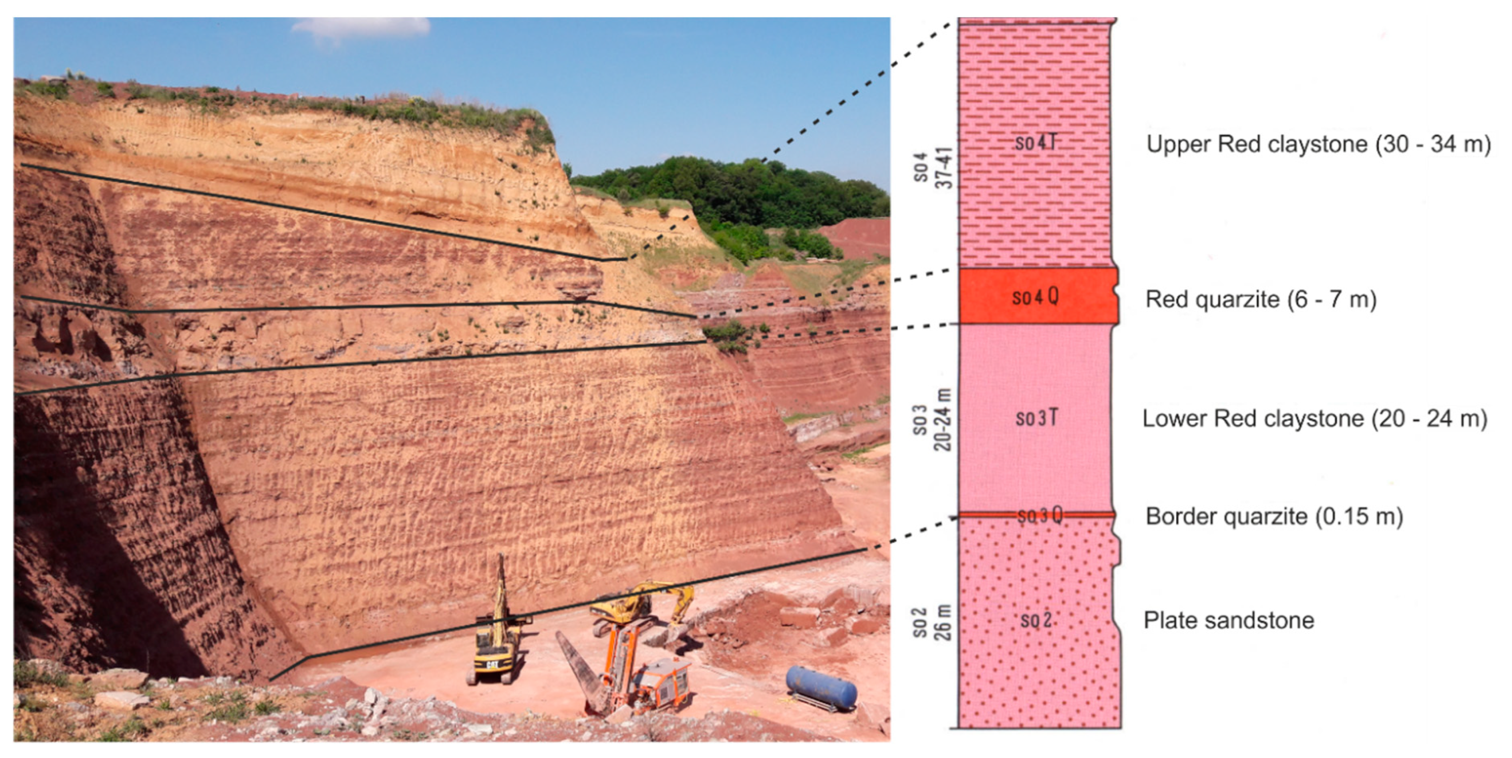
The Remlinger sandstone, which was used for the tests, was taken from a quarry in Remlingen near Würzburg (Bavaria, Germany). The quarry is operated by the company Seidenspinner Natursteinwerke (Location: 49°47′27.9″ N, 9°40′26.3″ E). The sandstone is a Triassic formation, which can be attributed to the Upper Buntsandstein and is found there in the area of the Thüngersheimer Anticline. Figure 1 shows a picture of the quarry and the stratigraphic sequence, related to the Upper Buntsandstein.

The Remlinger sandstone has a strong red color, but there are hardly any investigations in terms of properties and parameters. Therefore, the matrix permeability and porosity were determined for our specimens of the Remlinger sandstone. For this purpose, the specimens were first dried in the oven for 24 h to obtain their dry weight. Using a vacuum pump and a desiccator, a saturation of the pore space was then initiated over a period of an additional 24 h. After this time, the weight was measured again and the porosity was determined by a geometric volume calculation. The matrix permeability was determined by inserting the saturated specimens in a press and applying a triaxial stress state. The specimen was then flowed through and, by using the measured pressure difference before and after the sample, the matrix permeability was calculated. Results showed a porosity of 12.9% (±0.3%) on average. In terms of the permeability, we obtained a mean value of 5.50 × 10⁻¹⁷ m² (±8.24 × 10⁻¹⁸ m²). Within the scope of an optical inspection, the Remlinger sandstone looks fine grained, very homogeneous and isotropic (see Figure 2).

Specimens for the flow-through experiments were drilled, sawed and fractured perpendicular to the stratification of the bored sandstones. The exception here is the naturally fractured specimen (Figure 2d), which was drilled with the drill rig in the direction of the stratification due to the limited accessibility of a fractured wall in the quarry. The self-produced fracture (Figure 2c) was created by a Brazilian test using a splitting wedge extending over the length of the specimen. This wedge was chosen to obtain the straightest possible fracture through the specimen and to avoid splintering. In the following, sandstone specimens are labelled as sawed Rem_sw, split Rem_sp and natural Rem_na.

The sandstone specimens have a length of 150 mm (y direction), a diameter of 100 mm (x direction) and a single fracture, which runs from the bottom to the top along the long side of the middle of the specimen. The specimen halves were marked (red and black) for the identification and then re-combined without any shear displacement. During the sawing and splitting of the specimen, minor material loss along the fracture surface was unavoidable.

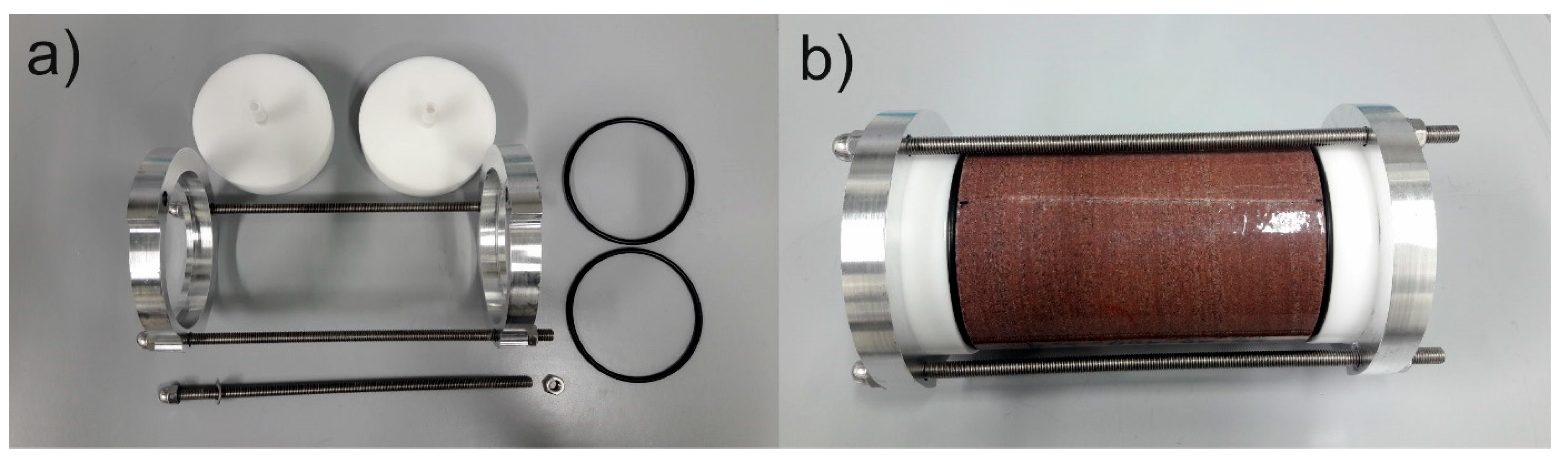
To prepare the flow experiments, the specimens were covered with a thin Teflon shrinking tube (PTFE 400—101.6/25.4 mm (4″)—nature, wall thickness before shrinkage approx. 0.1 mm), so that a displacement of the specimens during the experiments is prevented but flow through the specimen’s fracture is unrestricted. The shrink tube protruded approx. 1 cm over the upper and lower side of the specimen to achieve maximum sealing with the sealing rings when the specimen was inserted into the clamping device for the flow experiments (Figure 3).

Before the start of the experiment, the specimens were saturated over a period of at least 12 h in a desiccator connected to a vacuum pump. As saturation fluid distilled water was used, which was preconditioned 7 days before with crushed material of the corresponding sandstone under temperature influence (90 °C) on a shaking table. The preconditioning was carried out in order to minimize the water–rock interaction.

The coated specimens were then inserted into the clamping device. For this purpose, two sealing rings (P 583/NBR 70, diameter 90 mm, cord thickness 4 mm) were used on the top and bottom of the specimens, each followed by a Teflon attachment, which was provided with a tube connection. The Teflon attachments were slightly conical on the underside (inclination approx. 3°) so that water can flow without turbulences and dead water volume. The sealing rings lay on the overlapping shrink tubing. Using a specially manufactured clamping device consisting of two aluminum rings and three clamping screws (angle 120° to each other), the Teflon attachments were then pressed onto the sealing rings and the specimen to seal the system. Then, the tubes were attached to the inlet and outlet of the Teflon attachments and the system was put into operation.

2.2. Experimental Setup

The flow experiments to determine the hydraulic parameters (permeability, fracture aperture, dispersivity, velocity, dispersion coefficient) were carried out using a simple Darcy test setup (Figure 4) with distilled, vented water. For this purpose, distilled water was connected to a vacuum pump in a desiccator and a negative pressure was applied until no more air bubbles formed. This was usually achieved after 4 to 5 h. The vented water was then filled into storage tanks, from where it was inserted into the overflow tank and from there it flows through the experimental set-up. The overflow tank was used to set a constant water level. The inlet pressure level was controlled using a 3 m-long stand rod on which the overflow tank was attached. Afterwards, the water flowed through tubes to the fractured specimen, which was clamped in the special device (Figure 3). The tubes have been arranged in a way, so that a flow through the specimen took place from bottom to top, allowing any air captured in the fracture or pores that has accumulated during the process between removal from the desiccator for saturation and installation in the clamping device for the experiments, to escape easily. After the water had passed through the specimen and left at the top, it was led into a holder, which was also manufactured for these experiments. A sensor for the continuous measurement of the electrical conductivity as well as an outlet tap were attached to the holder, so that the water could be led from there into a collecting tank. The sensor used was a WTW Multi 3510 (Xylem Analytics Germany Sales GmbH & Co. KG, WTW, Weilheim, Germany) measuring instrument and an associated Tetracon 925c conductivity sensor (measuring accuracy for electric conductivity 0.5% of the measured value and 0.1 °C for temperature). The water outlet of the holder also determined the outlet pressure level so that, in combination with the level in the overflow tank, the hydraulic gradient could be defined. The measurement of the flow rate to determine the hydraulic permeability and fracture aperture was carried out using a laboratory balance (accuracy 0.01 g). To determine further hydraulic rock parameters (dispersivity, velocity, dispersion coefficient), tracer experiments were carried out. For these, a sodium chloride solution was injected just before the specimen and the change in the electrical conductivity was recorded after the water left the specimen.

2.3. Experimental Procedure

Darcy experiments were done to ensure a constant fluid flux through the fracture so that the tracer experiments could be carried out. For this purpose, the amount of water which flowed through the system in a corresponding period of time was determined at regular intervals using the available laboratory scale until it achieved a constant outflow. The time intervals were kept as short as possible (1 min if possible) in order to record even the smallest changes. Afterwards, the tracer experiments were carried out to determine the transport parameters, namely velocity, dispersivity, dispersion (compare Chapter 2.5). For all tests, identical settings were used for the Darcy and tracer tests if possible, related to the hydraulic gradient to ensure comparability between all specimens. We adjusted a pressure difference dh of approx. 0.7 m over the specimen length dx of 0.15 m, resulting in a hydraulic gradient I(x) = 4.67 for the sawed and split specimen. For the naturally fractured one, however, the hydraulic gradient was reduced, since the large opening width would otherwise have resulted in very large Reynolds numbers. Here, a pressure difference of only 0.15 m over the specimen length was set, resulting in a hydraulic gradient I(x) = 1.0.

For the tracer tests, 1 mL of a two-molar sodium chloride solution was injected as near as possible in front of the specimen as a Dirac pulse (injection time ~1 s) and the resulting increase in electrical conductivity was measured every second using the previously described sensor at the water outlet. As in the Darcy experiments, the amount of water used during the experiment was collected and weighed to calculate further measures such as tracer recovery.

2.4. Determination of Hydraulic Parameters

To ensure laminar flow conditions, the dimensionless Reynolds number Re (-) was determined for the tests. The calculation was done after [43]:

$$Re=\frac{2\times Q}{{\nu }_{kin}\times L_W}=\frac{2\times Q\times \rho }{\mu \times L_W}$$

(1)

by the relation of the flow rate Q (m³/s), the kinematic viscosity ν_kin (m²/s), the dynamic viscosity µ (kg/m s), the density ρ (kg/m³) and the fracture width L_W (m). In the literature, there is much discussion for fractured systems about the upper limit of the Reynolds number for laminar flow. Reynolds numbers between <1 [44], over 50 [45] and 90 [46] up to 2000 [47] are given as limits.

A transformation of the Navier-Stokes equation leads to the cubic law [43], which can be described as

$$Q= \frac{\rho \times g\times dh}{L_L}\times \frac{a_{eff}^3}{12\times \mu }\times L_W$$

(2)

with gravitational acceleration g (m/s²), hydraulic pressure difference dh (m) and the aperture length in flow direction L_L (m). By transforming the cubic law (Equation (2)), we calculated the equivalent hydraulic aperture or cubic law aperture width a_eff (m) [43,48] by

$$a_{eff}= \sqrt[3]{\frac{12\times \mu \times Q}{\rho \times g\times \frac{dh}{L_L}\times L_W}}=\sqrt[3]{\frac{6\times \mu ²\times Re}{{\rho }^2\times g\times \frac{dh}{L_L}}}$$

(3)

The intrinsic permeability was calculated by the Darcy Law [49,50,51]:

$$q=-k\times I$$

(4)

where q (m/s) is the specific flow rate, k (m/s) the hydraulic conductivity and I (-) is the hydraulic gradient. Replacing the specific flow rate by the relationship between the flow rate and the cross-sectional area A (m²), and the hydraulic gradient defined as a difference in piezometric head dh over flow distance dx, and as the flow distance dx matches the gap length in the flow direction L_L (m), it follows

$$Q=-k\times A\times \frac{dh}{L_L}$$

(5)

From the comparison of Equations (2) and (5), the hydraulic conductivity k (m/s) can be calculated by [43]

$$k=\frac{\rho \times g\times {a_{eff}}^2}{12\mu }=\frac{g\times {a_{eff}}^2}{12{\nu }_{kin}}$$

(6)

The intrinsic permeability K (m²) results after [52] by

$$K=\frac{{a_{eff}}^2}{12}$$

(7)

Equations (1), (3) and (7) were used to determine the flow regimes and to calculate the equivalent hydraulic fracture aperture and permeability. In order to determine the transport parameters, the output curves of the tracer tests were fitted by using the Continuous Time Random Walk method (CTRW) and the advection–dispersion equation (ADE) (see Section 2.5).

For the correct calculation of the transport parameters, both a temporal shift of the breakthrough curves and a mixing effect after the tracer left the specimen would need to be considered. The time shift results from the experimental set-up, because the electrical conductivity is not measured directly at the end of the specimen, but several centimeters behind. Since the degree of mixing in the outlet volume cannot be determined, only the temporal shift of the breakthrough curves is calculated. Based on the comparably high flow velocity and the conical shape of the setup, we assumed that only minor mixing effects take place in the volume between the specimen and sensor. In order to be able to calculate the concentrations of the breakthrough curve, a calibration curve was created which was used to convert the measured electrical conductivities into a concentration.

The calibration curve was generated by preparing NaCl solutions of different concentrations (0.001 to 0.02 mol/L) and then measuring the electrical conductivity of those. We achieved a linear regression between concentration c and the electric conductivity EC by (c (g/L) = 5.0523 × 10⁻⁴ × EC (μS/cm)) with R² = 0.9997.

2.5. Determination of Transport Parameters

In the classical approach, assuming a steady state laminar flow situation with no retardation or reaction, the tracer concentration is described by the advection–dispersion equation (ADE). Simplifying the fracture flow to a one-dimensional problem, the ADE of a tracer concentration c (kg/m³) over time t (s) in the flow direction y can be written as

$$\frac{\partial c}{\partial t}=-v\frac{\partial c}{\partial y}+D_L\frac{{\partial }^{2}c}{\partial y^2}$$

(8)

with transport velocity v (m/s) and dispersion coefficient D_L. The analytical solution to this equation for a pulse injection of length t₀ (s) and no initial concentration is given by [53]

$$c\left(x,t\right)=c_0\times A\left(x,t\right)-c_0\times A\left(x,t-t_0\right),$$

(9)

with the pulse concentration c₀ (kg/m³) and:

$$A\left(x,t\right)=\left(\frac{1}{2}erfc\left[\frac{x-vt}{2\sqrt{D_{L}t}}\right]+\frac{1}{2}\exp \left(\frac{vx}{D_L}\right)erfc\left[\frac{x+vt}{2\sqrt{D_{L}t}}\right]\right)$$

(10)

The analytical solution is fitted to the experimental BTCs using the least square fit routine provided by Matlab to obtain the best fit for transport velocity v and dispersion coefficient D_L at x = 0.15 m, representing the specimen end. The least square fit was conducted with a function and step size tolerance of 10⁻⁹ and the fit was completed or aborted once one of those criteria was reached. The residual norm of the fit was calculated as the squared 2-norm of the residual.

However, through the usually strong non-Fickian transport behavior indicated through multiple peaks and the long tailing of the BTC, the ADE often results in an insufficient match of the transport parameters [38]. Previous studies showed that the continuous time random walk (CTRW) method is able to reproduce those non-Fickian features superior to a fit of the ADE (e.g., [25,26]). The CTRW is based on a Laplace transformation of the ADE using a memory function M [54]. In a one-dimensional Laplace space, the transport equation of a concentration c(x,u) at a space x and for a Laplace variable u (1/s) can be written as

$$uc\left(x,u\right)-c_0\left(x\right)=-M\left(u\right)\left[v\frac{\partial }{\partial x}c\left(x,u\right)-D\frac{{\partial }^2}{\partial x^2}c\left(x,u\right)\right],$$

(11)

with initial concentration c₀, transport velocity v, dispersivity D and memory function:

$$M\left(u\right)=t_{char}u\frac{\phi \left(u\right)}{1-\phi \left(u\right)},$$

(12)

using a characteristic time t_char and the function φ. The memory function represents microscopic heterogeneities along the flow path and has various shapes, depending on the function φ. Most commonly, a truncated power law (TPL) is used in the form of:

$$\phi \left(u\right)={\left(1+{\tau }_{2}u{t}_1\right)}^{\beta }\exp \left(t_{1}u\right)\mathsf{\Gamma }\left(-\beta , {\tau }_2^{-1}+t_{1}u\right)/\mathsf{\Gamma }\left(-\beta , {\tau }_2^{-1}\right),$$

(13)

introducing three additional input parameters β, t₁ and t₂, as τ₂ = t₂/t₁. Here, t₁ is the transition time and marks the beginning of the power law behavior, while t₂ is the cut-off time [55]. The value of β has previously been linked to fracture heterogeneity [27] and the Hurst exponent [24]. An analytical solution of Equation (11) can be derived for a specified memory function M, fitted to experimentally obtained BTCs and then transformed back to the time domain. It is noteworthy that all parameters in Equation (11) are given in the Laplace space and need to be transformed. The whole procedure was done using the CTRW Toolbox (version 4.0) for Matlab (The Mathworks, Inc., Natick, MA, USA) provided by [56]. An in-depth discussion of the used numerical and mathematical background can be found in [56] as well as in the manual of the toolbox itself. In a first trial and error approach, starting values were obtained that achieved a visually decent fit. The obtained values were used as starting values for the subsequent minimization process with a function and step size tolerance of 10⁻⁹.

2.6. Characterization of Fracture Roughness

Scans of the fracture surfaces were performed prior to reassembling using the scanner NextEngine ScanStudio PRO and the highest possible resolution of 17,000 data points per square-inch. Data processing was done using Matlab, including the interpolation of scanned points onto a regular grid without a loss in data point density. Relative height values to a mean reference plane were calculated based on the absolute height values.

To quantify the roughness of a fracture surface, several methods were common, such as Gaussian statistics of the height distribution [57], fractal parameters [58] and the joint roughness coefficient (JRC), which has been especially popular in engineering geology [59].

Besides the mean values and spread of the relative heights dz distribution, the skewness and kurtosis of the distribution can be calculated. The skewness sk:

$$sk=\frac{1}{{\sigma }^{3}N}\sum _{i=1}^{N}d{z}_i^3$$

(14)

for a height profile with N points and a standard deviation σ is a measure of the symmetry of a distribution, which is zero for a symmetric distribution [57]. The kurtosis K is a measure of the sharpness of the distribution. As a reference, the K of a normal distribution is three. The kurtosis of a distribution sharper than the normal distribution is smaller than three and vice versa. The kurtosis is calculated as [57]

$$K=\frac{1}{{\sigma }^{4}N}\sum _{i=1}^{N}d{z}_i^4.$$

(15)

In this work, skewness and kurtosis were calculated for the separate specimen halves [57]. In addition to the statistical analysis, key measures of the amplitude and its spatial spreading can be determined. One of those key measures is the total height R_t, which is the difference of the maximum peak height R_p and the minimal valley depth R_v of the relative heights [60]. The spatial spread can be quantified e.g., by the peak density N_p and the zero-crossing density N₀, which account for the numbers of peaks and zero-crossings along the profile length [60].

As fractal parameter, the Hurst exponent relates the scale of height parameters with the spatial dimension it is observed on. The Hurst exponent can e.g., be determined by splitting a profile of the length L in bands with defined lengths db. As long as db < L/2, there are several bands along the profile. For each band, the height difference between the minimum valley and maximum peak is determined and the mean value of all bands with an equal length db is calculated. Plotting the band length db versus the corresponding mean values usually results in a linear curve, whose inclination can be determined through a linear fit using intrinsic Matlab function polyfit() and the inclination is equal to the Hurst exponent [61]. There have been attempts to relate the Hurst exponent with the JRC but the method of determining the Hurst exponent has been shown to have a substantial influence on this relationship (e.g., [62,63]).

The JRC of a surface can be determined by various methods, making it a very popular quantity to be used in laboratory studies as well as in numerical simulations (e.g., [64,65,66]). Additionally, the JRC value can be linked to the Z₂ value for a quantitative determination (e.g., [30]). The Z₂ value can be obtained for individual profiles requiring the splitting of the surface into discrete profiles. This method allows the assessment of anisotropy by defining profiles in two orthogonal directions, e.g., in the direction of the pressure gradient and vertical to it. For a profile consisting of N data points and each point i marked by a position x_i and a relative height value dz_i, the Z₂ value is calculated as [30]

$$Z_2=\sqrt{\frac{1}{N}{\displaystyle \sum }_{i=1}^N{\left(\frac{d{z}_{i-1}-d{z}_i}{x_{i-1}-x_i}\right)}^2}$$

(16)

from which the JRC value can be calculated as

$$JRC=32.2+32.47\log \left(Z_2\right).$$

(17)

While all previously described parameters are usually determined for a profile, there are surface measures trying to capture the characteristic of a whole two-dimensional surface in a single quantity. The Z_2s value is one of such quantities, which besides the one-dimensional formulation, Z₂ along a profile can also be calculated for a two-dimensional surface Z_2s by extending Equation (16) to [67]:

$$Z_{2s}=\sqrt{\frac{1}{\left(N_x-1\right)\left(N_y-1\right)dxdy}\left[{\displaystyle \sum }_{i=1}^{N_x-1}{\displaystyle \sum }_{j=1}^{N_y-1}{\left(d{z}_{i+1,j}-d{z}_{i,j}\right)}^2+{\left(d{z}_{i,j+1}-d{z}_{i,j}\right)}^2\right]}$$

(18)

with N_x and N_y points in x and y direction spaced by dx and dy, respectively.

3. Results

3.1. Determination of Hydraulic Parameters

Three tracer and Darcy tests were carried out on each specimen under similar conditions to determine the hydraulic and transport-relevant parameters of the fractures. The Darcy tests were used to determine the equivalent hydraulic aperture and the Reynolds number, and conclusions were drawn from the tracer tests regarding dispersivity, dispersion and flow velocity in the fractures using a CTRW fit to the measured breakthrough curves, where these parameters were used as fitting parameters, among others. For each specimen, the three tracer tests were performed under identical conditions (see Section 2.3) to prove the reproducibility of the experiments. Figure 5 shows the measured breakthrough curves of all three tests conducted for the three differently fractured specimens (a–c) and a direct comparison of the breakthrough curves (d).

For each specimen, the three repetitive tests show a good agreement with minor divergences between the three tests compared to the significant differences that can be seen at the BTCs of the different fractures. Variations between the three repetitive tests can be caused by the injection process, but also by unavoidable vibrations of the experimental setup, e.g., due to air movement. For example, the small concentration peak seen in Figure 5b after 1100 s was only observed in Test 1 and therefore most likely caused by an unknown systematic error rather than a physical process, such as channeling effects, as it is non-reproducible.

The sawed specimen experienced the greatest differences among the three BTCs of all the tested specimens. It also had the highest concentration peaks followed by the naturally fractured specimen and the split specimen. It is noticeable that the natural fracture shows the smoothest BTCs while the split specimen had the “noisiest” BTCs, exhibiting high frequency variations on top of the general trend. Clear differences in the three specimens can also be observed with regard to the duration of the individual experiments. In contrast to the split specimen, where the flow-through tests took by far the longest, the tests were completed most quickly in the naturally fractured specimen. However, nearly the same fluid volume of approx. 1 L was used for the flow-through in all experiments. Therefore, in order to be able to show the differences in the breakthrough curves, the observed concentrations were plotted with respect to the volume that flowed through the fractures (Figure 5d). The comparison of the breakthrough curves of the three specimens showed that the first arrival of the tracer occurs with the smallest flow volume in the natural fracture, whereas the first arrival for the sawed and split specimen is almost identical. It can also be seen that the experiments on the fractured specimen show the greatest widening of the BTCs, followed by the natural fracture. The narrowest BTCs can be seen for the sawed specimen.

In order to determine the transport-relevant parameters for the different fracture types, a CTRW fit was adapted to the BTCs (Figure 6). The BTCs can be reproduced very well with the CTRW curves, even if the course deviates slightly from the measured values, especially in the area of the tailing. This is evident for the sawed (a) and split (b) specimen. For the naturally fractured specimen (c), on the other hand, hardly any significant deviations between the CTRW fit and the measured breakthrough curve can be visually detected. For all fits, the normalized error is below 2%.

The parameters listed in

Table 1. Hydraulic, transport and fitting parameters estimated from the Darcy and tracer experiments as well as the CTRW fits with standard deviation values.

Fracture Type Parameter	Sawed	Split	Natural
Reynolds number (-)	12.97 ± 0.38	4.62 ± 0.08	27.07 ± 0.30
Equivalent hydraulic aperture (µm)	117.29 ± 0.91	83.06 ± 0.65	248.58 ± 1.38
Dispersivity (m)	1.65 × 10−2 ± 5.98 × 10−3	3.16 × 10−2 ± 1.67 × 10−3	5.50 × 10−2 ± 1.39 × 10−3
Velocity (m/s)	2.34 × 10−3 ± 2.37 × 10−4	1.13 × 10−4 ± 7.97 × 10−6	2.36 × 10−3 ± 5.60 × 10−6
Dispersion coefficient (m²/s)	3.85 × 10−5 ± 3.83 × 10−6	3.58 × 10−6 ± 2.93 × 10−7	1.30 × 10−4 ± 4.43 × 10−6
β value (CTRW)	5.47 ± 1.25	3.25 ± 1.05	10.71 ± 0.65

result from the Darcy tests and the CTRW fits to the breakthrough curves measured in the tracer tests. It is noticeable that the split specimen has the smallest equivalent hydraulic aperture of approx. 83 µm. For the sawed specimen, this could be determined to be approx. 117 µm and for the natural fracture to be around 248 µm. The Reynolds numbers are between 4.6 and 27.

For the transport parameters, the dispersivity is 1.65 × 10⁻² m (±5.98 × 10⁻³ m) for the sawed specimen to 5.50 × 10⁻² m (±1.39 × 10⁻³ m) for the naturally fractured one. For the split specimen, the dispersivity is around 3.16 × 10⁻² m (±1.67 × 10⁻³ m). The determined flow velocities are quite comparable with 2.34 × 10⁻³ m/s (±2.37 × 10⁻⁴ m/s) and 2.36 × 10⁻³ m/s (±5.60 × 10⁻⁶ m/s) for the sawed and natural fracture, respectively, although the hydraulic gradient for the natural fracture was chosen to be significantly lower due to its large equivalent hydraulic aperture. The flow velocity for the split specimen of 1.13 × 10⁻⁴ m/s (±7.97 × 10⁻⁶ m/s) is significantly smaller, agreeing with the longer duration of the experiment. The dispersion coefficient is the smallest with 3.58 × 10⁻⁶ m²/s (±2.93 × 10⁻⁷ m²/s) for the split, intermediate, with 3.85 × 10⁻⁵ m²/s (±3.83 × 10⁻⁶ m²/s) for the sawed and highest with 1.30 × 10⁻⁴ m²/s (±4.43 × 10⁻⁶ m²/s) for the natural fracture. Noticeable is the evolution of the fitting parameter β of the TPL, which is smallest with approximately 3 for the split specimen, around 5.5 for the sawed specimen and almost 11 for the natural fracture.

The least square fit of the ADE results in comparable numbers to the CTRW values for the natural and sawed fracture with respectable small residual norms (

Table 2. Transport parameters obtained through the advection–dispersion equation (ADE) fit with the standard deviation values.

Fracture Type Parameter	Sawed	Split	Natural
Dispersivity (m)	1.62 × 10−2 ± 1.09 × 10−3	5.15 × 10−2 ± 8.23 × 10−3	4.29 × 10−2 ± 1.99 × 10−3
Velocity (m/s)	1.41 × 10−3 ± 1.61 × 10−4	2.49 × 10−4 ± 4.04 × 10−5	2.48 × 10−3 ± 9.44 × 10−5
Dispersion coefficient (m²/s)	2.27 × 10−5 ± 1.04 × 10−6	1.26 × 10−5 ± 1.24 × 10−6	1.06 × 10−4 ± 3.44 × 10−6
Residual norm (-)	0.75 ± 0.08	7.17 ± 0.74	0.84 ± 0.14

). On the other hand, the split specimen results in a poor-quality fit using the ADE with substantially larger residual norms for the ADE fit compared to the norms achieved by the sawed and naturally fractured specimens. Furthermore, also visually, the inability of the ADE to match the long tailing of the BTC of the split specimen is especially obvious (Figure 7). For the sawed and natural fracture, visually there is no observable difference between the ADE and CTRW fit, as can be expected from the small differences in the obtained parameter values.

3.2. Fracture Roughness

The relative height distribution of the sawed specimen halves is slightly sharper than the normal distribution with a mean kurtosis of 2.8 (Figure 8a). The total amplitude R_t is around 0.47 mm and the mean peak height R_p is around 0.21 mm for both specimen halves. The mean valley height R_v is around −0.25 mm but one specimens halve is around −0.21 mm and the other one is around −0.29 mm. No anisotropy was observed in the amplitude parameters. In the spatial parameters, such as peak density N_p, there is anisotropy with 1.41 mm⁻¹ in flow and 0.6 mm⁻¹ x direction. The zero-crossing density N₀ is lower than the peak density but exhibits a similar anisotropy with roughly 0.59 mm⁻¹ in the flow direction and 0.38 mm⁻¹ in the x direction. The JRC analysis reveals intermediate roughness parameters with mean values varying around 4 in the flow direction and 7 in the y direction with little differences between both specimen halves. The Hurst exponent has a similar anisotropy, with 0.49 in the flow direction and 0.42 in the x direction. The surface Z_2s value is almost equal for both specimen halves with 0.25 and 0.24, respectively.

The relative height distribution of the split specimen is close to a normal distribution, as can be seen from the skewness of the relative height distribution, which is 0.11 (Figure 8b). The kurtosis of the relative height distribution is around 2.4 indicating a sharper distribution compared to the normal distribution. The total amplitude height is around 3.63 and 3.80 mm for the flow and x directions, respectively, with minor variations between the specimen halves. Mean peak and valley heights are similar in amplitude around 1.84 mm with negligible variations between the directions and specimen halves. Anisotropy is again observable in the spatial parameters with a peak density N_p of 0.79 mm⁻¹ and 0.42 mm⁻¹, as well in the zero crossing density N₀ of 0.11 mm⁻¹ in the flow and 0.05 mm⁻¹ in the x direction. The JRC value has comparably little anisotropic behavior with a JRC of 12.39 in the flow and 12.00 in the x direction, in contrast to the other values which represented a larger roughness in the x than in the flow direction. The Hurst exponent is similar for both directions and specimen halves with a value of 0.77. The surface Z_2s value is 0.35 for both specimen halves.

The natural fracture shows anisotropy in the flow direction and vertical to it for almost all surface roughness measures. As an example, the skewness of the relative height distribution of the surfaces is obtained as 0.49 in the flow and 0.24 in x direction. The kurtosis of the relative height distribution is with approximately 2.7 smaller than 3 for both halves and directions, indicating a sharper distribution than the normal distribution (Figure 8c). The total amplitude R_t is 1.3 mm in the flow and 1.7 mm in the x direction. The mean maximum peak height R_p varies between 0.56 mm in the flow direction and 0.78 mm in the x direction for one half. For the other specimen half, the R_p values vary between 0.78 and 0.93 mm. A similar spread and distribution was also obtained for R_v. The spatial roughness parameters also exhibit strong anisotropy close to 2, with Np approximately 1.22 mm⁻¹ in the flow and 0.60 mm⁻¹ in the x direction. The zero-crossing density N₀ is smaller than N_p for all the specimen halves and directions, with 0.36 and 0.18 mm⁻¹ in the flow and x directions, respectively. The more comprehensive roughness parameters, such as the JRC coefficient, reveal a similar trend with strong anisotropy. The mean JRC value in the flow direction is 12.67 and in the x direction is 18.26. The difference between the specimen halves is around 1.2 for both directions. The Hurst exponent is 0.61 in the flow and 0.55 in the x direction as mean value of both halves. The surface Z_2s value is 0.48 and 0.44 for the halves, respectively. The relative height distributions in comparison for both specimen halves of each of the different fracture types are shown in Figure 9.

4. Discussion

The comparison of the fracture surfaces of the three specimens reveals distinct differences between the fracture generation processes. The natural fracture possesses the most anisotropic behavior across all calculated surface measures. The natural fracture is also characterized by significant differences between both specimen halves. This indicates either a complex generation process probably including a large shear displacement so that the fracture halves are not matching, or weathering processes along the fracture surface with the precipitation and dissolution processes of minerals, or a combination of both. This might also explain the comparably large equivalent hydraulic aperture although the obtained roughness amplitude parameters are in the medium range of the three specimens and the JRC is also comparable to the split specimen. Compared with roughness, the overall quantities of the natural and split specimen are inconclusive. While the surfaces of the split specimen have the lower JRC and Z_2s values, it has the higher Hurst exponent compared to the natural fracture. However, the differences are rather small. With respect to the spatial and amplitude parameters, the natural and split specimens are obviously different as the split specimen has the narrowest relative height distribution of all three tested specimens, both specimen halves are very similar and the amplitudes are almost three times as large in the split fracture as in the natural fracture at an almost similar peak density. Only the spatial parameters reveal some anisotropy for the split specimen with higher peak densities in the flow than in the x direction, though this anisotropy does not substantially affect the JRC. The observed behavior is in good agreement with the fracture generation process as both specimen halves were split from the same intact specimen and only unavoidable material loss causes separation and differences between the halves. For the hydraulic tests, the specimen halves were joined together without any shear displacement, causing a very narrow equivalent hydraulic aperture.

Obviously, the sawed specimen was the one with the smallest amplitude, the smallest JRC, the smallest Z_2s and the smallest Hurst exponent. All those parameters characterize the sawed fracture surface as the smoothest one of the surfaces tested. The specimen halves are also very similar and only in the spatial parameters was anisotropy observed as well as in the JRC. This anisotropy might either be caused by the direction of sawing and by the orientation of the teeth of the saw blade or represent a natural anisotropy. Although the fracture surfaces are rather smooth, the observed equivalent hydraulic aperture is comparably large. It is visible, that through the sawing, the specimen halves slightly deform at each end as stress is released due to the generated fracture. Due to this stress release, the specimen halves are apart at both ends of the specimen causing a slight but visible and observable increase in fracture aperture that is also hydraulically effective. This deformation does not occur in the split specimen, as the fracture occurs along natural weak points in the specimen and has a macroscopic tortuosity that the sawed fracture cannot have due to its generation process. However, also inaccuracy and an increased amount of material loss during sawing cannot be completely eliminated, possibly contributing to the larger aperture at each end of the sawed specimen.

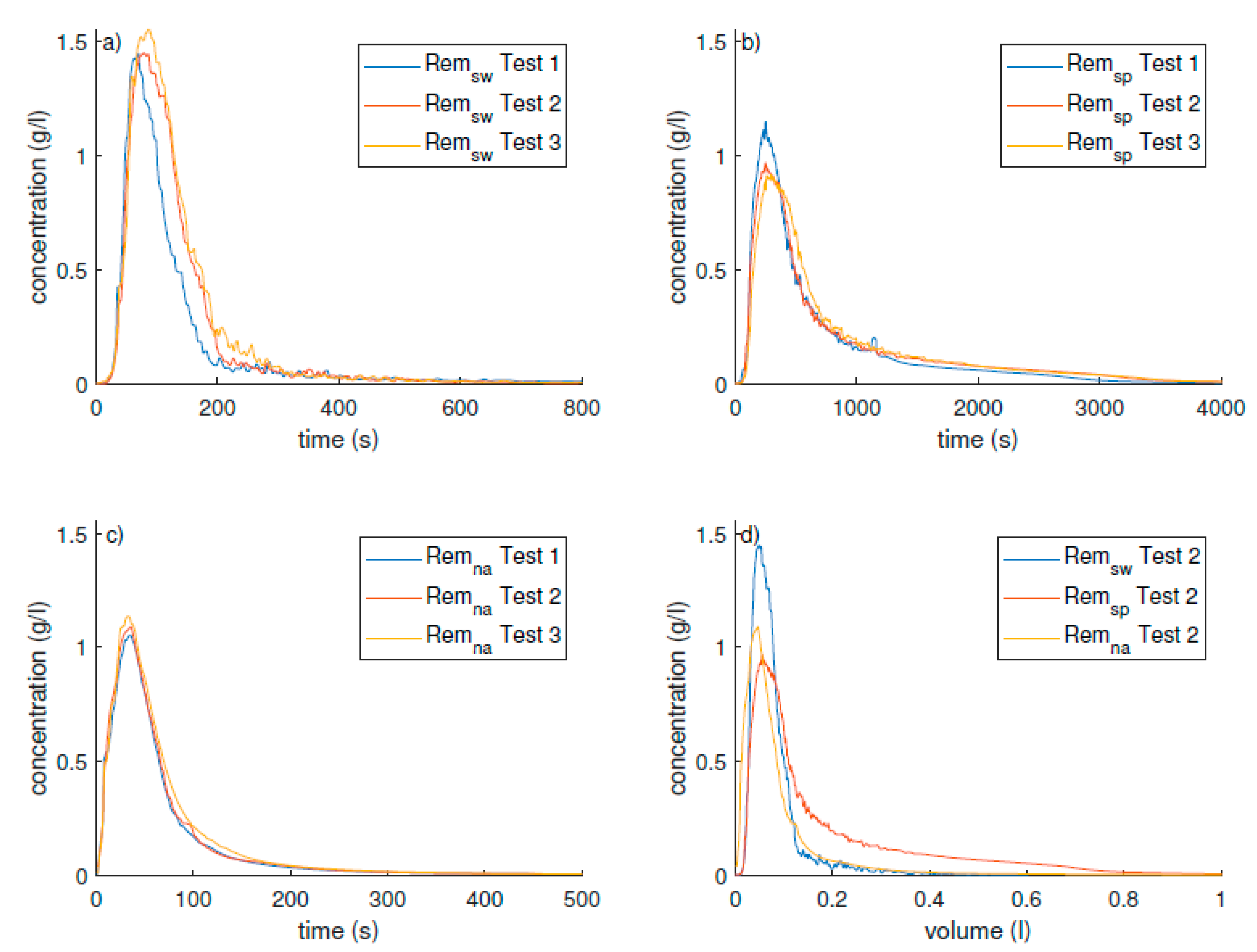
A direct comparison of the BTCs shown in Figure 5 allows to consider all tests as reproducible and representative, as all three tests of each specimen reveal a similar shape and only diverge negligibly. The calculated Reynolds numbers for each experiment are below the considered limit of 30 for the transition from laminar to turbulent flow [45], so that the laminar flow can be considered and the cubic law can be applied for the calculation of an equivalent hydraulic aperture. The flow velocities, one equivalent value for the calculation of the Reynolds number, correlate with the calculated effective hydraulic apertures achieving higher flow rates in fractures with a larger equivalent hydraulic aperture. However, one needs to keep in mind that the hydraulic gradient for the natural fracture was reduced significantly to assure the sufficient duration of the experiment limited by the measurement frequency of the used instrumentation. A further reduction was not achievable as the smallest gradient over specimen length was already set.

As the dispersion coefficient is the product of velocity and dispersivity, the following discussion of the transport behavior focuses on the dispersivity as independent parameter due to the diverging velocities within the separate fractures. For now, we will stick to the results of the CTRW fit. The sawed specimen, with the smoothest surface, also shows the lowest dispersivity. The lack of substantial surface morphology results in a minimal influence on the tracer path and retardation due to the lack of asperities and resulting tortuosity or curls. This agrees well with the analysis of the BTCs of the sawed specimen, showing the highest concentration peaks, the shortest tailing and the narrowest shape. For the split specimen, the calculated dispersivity is as twice as large and for the natural fracture the dispersivity is another 1.7 times larger. The larger dispersivity of the split specimen compared to the sawed one might be explained by the significantly larger surface roughness and the resulting retardation and more complex flow paths. However, the surface roughness from split and natural specimen is quite comparable, not by itself explaining the larger dispersivity of the natural fracture. Considering the larger Reynolds number as well as the anisotropy with an increased roughness vertical to the flow direction in the natural fracture, a potentially non-linear flow behavior might cause an increased dispersion in the natural fracture causing mixing effects along the flow resulting in larger dispersivities and lower peak concentrations of the tracer, but not further increasing the tailing of the BTCs. However, the fitting parameter β of the TPL in the CTRW was previously used as an indicator for non-Fickian transport processes [24] and linked to contact area and Hurst exponent. However, the obtained parameters by [24] and [25] for β were smaller than 2, which is also given as a limit by [56] for Fickian transport. Our study shows, that for values of β larger than 4, the ADE is a suitable description and differences between fitting parameters of CTRW and ADE are within the range of fitting accuracy. This indicates, that for the sawed and natural fracture, non-Fickian transport, and therefore also nonlinear flow behavior, is negligible despite of the comparably large Reynolds numbers. For the split specimen, however, although β = 3.25, non-Fickian transport seems relevant as the ADE falls short to reproduce the long tailing of the experimentally obtained BTCs. Based on this argumentation, the hypothesis of non-Fickian transport processes causing the comparably large dispersivity of the natural fracture compared to the split specimen is rejected. The strong divergence between the fracture halves and the large anisotropy of almost all roughness measures of the natural fracture seem therefore responsible for the larger dispersivity of the natural fracture compared to the split fracture despite their similar surface roughness.

Surface roughness is known to cause channeling of the flow field. The BTCs of the split specimen exhibited high frequency variations on top of the general decaying trend of the BTCs. Those can be explained through channeling effects as separate channels can cause small concentration peaks as the tracer might be delivered batch wise on those microscopic channels. The flow channels also cause retardation effects due to tortuosity resulting in a longer tailing of the BTCs as observed for the split specimen. The BTCs of the natural fracture, although of similar surface roughness, are significantly smoother. This agrees with previous studies indicating that the influence of surface roughness on channeling decreases with increasing fracture aperture [10,11,12]. In addition, the very high flow velocity and the short duration of the experiment might reduce the differences of the separate flow paths to a degree that they cannot be experimentally resolved. The BTCs of the sawed specimen, although comparably smooth, also exhibit high frequency variations of the concentration signal but to a much smaller degree than that of the split specimen. The intermediate equivalent hydraulic aperture, the existing slight roughness and the anisotropy might cause those variations towards the end of the tailing.

A relationship between β and the Hurst exponent cannot be observed. However, only β values larger than that considered by [24] were obtained in this work and the correlation to the Hurst exponent started to vanish in [24] using numerical models. In general, no simple correlation between any roughness parameter, such as JRC or Hurst exponent, and a transport parameter (neither from ADE or CTRW) has been found in this work. The smoothest fracture surface (small JRC, Z_2s and Hurst exponent) has an intermediate equivalent hydraulic aperture and the smallest dispersivity, but an intermediate β value indicates Fickian transport. The split specimen has a comparably large surface roughness similar to the natural fracture but the dispersivity of the split specimen is almost half of the dispersivity calculated for the natural fracture, which also has an almost twice as large equivalent hydraulic aperture. The split specimen shows non-Fickian transport behavior while the natural fracture does not. Therefore, as anticipated, the contaminant transport process is multi-parameter dependent and therefore influenced by various features of the fracture surface morphology, such as the anisotropic behavior and congruence of the fracture surfaces, as well as by fracture aperture and flow velocity. Nevertheless, further experiments with a larger number of samples are required to verify and generalize the results.

5. Conclusions

Tracer tests have been conducted in three different types of single fractures in sandstone specimens. Additionally, the fracture surfaces have been scanned to analyze the surface morphology of sawed, split and natural fractures. Remlinger sandstone is a homogeneous type, with a small grain size and a surface with a JRC of 4–5 for the sawed and in the range of 12–13 for the split and natural fractures.

• Due to the slight deformation of the specimen halves at the specimen ends, the sawed fracture is not as narrow as the split specimen despite its small roughness amplitudes and well matching specimen halves. The smoothest fracture surface corresponds to the smallest dispersivity of all tested specimens, though slight anisotropy is observed probably caused by the sawing blade. The short tailing of the BTCs, with Reynolds numbers below 10, and good fit using the ADE and β > 5 indicate Fickian transport and linear flow.
• The split specimen has the largest roughness amplitudes with the smallest equivalent hydraulic aperture indicating well matching fracture surfaces without shear displacement. The bumpy BTCs give an indication of channeling effects caused by the large fracture roughness amplitudes. The channeling effects are much more significant here than in the other specimens. Comparably, small values of the CTRW fitting parameter (β ≈ 3.25) and a bad fit of the long tailing using the ADE reveal non-Fickian transport behavior. Previous studies indicated β ≥ 2 as the limit for Fickian transport.
• While the natural and split specimens have similar overall roughness parameters, there are substantial differences as the natural specimen has much smaller roughness amplitudes, is highly anisotropic in most roughness measures and both specimen halves reveal significant differences not observed for the other specimens. Those differences in the surface morphology of the specimen halves explain the largest equivalent hydraulic aperture as well as the largest dispersivity observed in the experiments. Comparably smooth BTCs indicate negligible channeling effects, agreeing with previous findings about the reduced influence of surface roughness on channeling effects with increasing fracture aperture.

The distinct differences between natural fractures and those generated through splitting question the representative nature of artificially generated faults with respect to surface morphology and the related hydrological processes. The shear displacements of split specimens, usually used to model natural fractures more realistically, might influence the local aperture distribution, but differences in surface morphology, such as anisotropy and roughness amplitudes, will persist and influence transport processes. While our work provides first insights into different transport behavior depending on fracture type and morphology, naturally, a larger sample size is required for a systematic study of the link between fracture surface morphology and contaminant transport, as well as to experimentally investigate transport processes in realistic fractures.