Drag Force Modeling of Surface Wave Dissipation by a Vegetation Field

Abstract

In this paper, we explore the use of coastal vegetation as a natural barrier to defend our shoreline from hazards caused by large wind waves, storm surges, and tsunamis. A numerical model based on XBeach is employed to evaluate the wave damping by vegetation. An explicit formula for the required drag coefficient used to help describe the additional force imposed by the vegetation is developed through a series of numerical experiments. Overall, our predictions agree reasonably with available laboratory data in the literature for various incident wave conditions and vegetation configurations. Our analysis suggests that a small unvegetated open space in the middle of a vegetation strip does not have a significant impact on the amount of wave height attenuation at the exit of the vegetated bed.

1. Introduction

Hard structures, such as sea dikes, breakwaters, and seawalls, have been widely built to protect our coastlines from wave attack. This common approach was proven to be quite effective in terms of short term coast protection. However, in the long run possible unfavorable domino effects are also shown due to the imposed forcing factors and the enforced boundary conditions by the building of the protection structures. Some usual disadvantages of hard structures are visual impacts, access restrictions, and reduced sand supply to beach. To achieve a balance between maintaining the shoreline functions and shielding the coast areas from wave impacts, soft engineering strategies have been increasingly recognized as a more environmentally sustainable approach to coastal protection. For instance, the ability of coastal vegetation buffer to reduce wave height and to protect the coast from erosion have been well recognized. By analyzing the pre- and post-tsunami satellite images, Danielsen et al. [1] showed that mangroves and coastal trees along the coast in the Cuddalore District, Tamil Nadu, India significantly reduced the damage caused by the devastating 2004 Indian Ocean Tsunami in the area. They observed that villages shielded by the coastal vegetation suffered only partial damage while those villages open directly to the coast were completely destroyed. In addition, satellite images also suggested that in this area only the first few rows of trees nearest to the shore were damaged during the 2004 tsunami event. In the more recent 2011 Japan Tōhoku Tsunami, the mitigation effects of coastal vegetation were also evident as Ranghieri and Ishiwatari [2] reported that the forested green belts (vegetated buffers) distributed along Japan’s sandy coast reduced the direct impact of the tsunami, delayed the wave inundation extended to the further inland, and protected the buildings by capturing debris drifted by the tsunami waves. They suggested that the effective protective role of the green belt can be generally categorized into the following: (1) The decrease of both tsunami wave energy and its propagation speed due to the dissipation by the wave-vegetation interaction; (2) The blocking of floating wreckage by the coastal trees reduces the direct impact of these obstacles on the built structures; (3) The holding of sand dune by vegetation roots enhances the dune’s ability to mitigate the tsunami wave impact force; (4) The firm-standing trees save the lives of people who are able to climb up or to cling to the trees. In addition to reducing tsunami damage, the protective functions of coastal vegetation (e.g., coconut trees, mangroves, salt marshes, and others) to weaken storm surges and associated coastal damages have also been supported by field data collected from cyclones and hurricanes. For example, to demonstrate the significant lifesaving effect of mangroves Das and Vincent [3] analyzed the number of storm-related deaths in several hundred coastal villages in the Kendrapada District, Orissa State, India during the 1999 super cyclone that struck the Orissa area. The 1999 category 5 cyclonic storm, which is probably one of the greatest cyclonic disasters in the 20th century, claimed nearly 10,000 deaths in total with more than 70% of them drowned by the surge. Based on their statistical analysis, Das and Vincent [3] argued that each hectare of mangrove forest saved 0.0145 lives during the cyclone and if there were no mangroves to shield the coast there would have been 1.72 additional deaths per village within 10 km from the shore in the 1999 event. In terms of the the economic value of coastal vegetation, Costanza et al. [4] studied 34 major hurricanes to strike the mainland U.S. since 1980 and estimated that, in 2008, coastal wetlands in the U.S. provide roughly $23 billion annually in storm protection services. In addition, they specified that coastal wetlands also produce a broad range of cultural ecosystem services and help preserve the natural character of the coastal environment, which hard coastal protection structures, such as vertical levees, are unable to account for.

On the basis of the above evidence, it is clear that, soft as they may seem, coastal green belts can be very effective to serve as a more environmentally sustainable barrier to buffer inland areas from daily waves, storm surges, and tsunamis. In this paper, our goal is to develop a numerical tool that can be used to model wave-vegetation phenomena for large-scale engineering problems. Indeed, many studies have been reported in the literature to evaluate the the effectiveness of such bio-shields. For instance, Massel, Furukawa and Brinkman [5] conducted field studies in both Townsville, Australia and Iriomote Island, Japan and observed that at high tide conditions the measured transmitted wave energy at two stations located 80 meters apart within the mangrove forest decreased roughly from 50% to 20% of the incident wave energy. Möller et al. [6] reported field measurements of wind waves at three locations across a sand flat to a coastal salt marsh on the coast of North Norfolk, England and showed that the wave energy dissipation over the salt marshes is about 2.5 times higher. Many laboratory studies have also been conducted to investigate the dynamics of wave-vegetation interaction. For instance, Luhar, Infantes, and Nepf [7] carried out wave tank experiment for seagrass motion under surface waves and showed that blade flexibility significantly reduced the hydrodynamic drag. Considering regular waves through flexible aquatic vegetation in a 18 m long wave flume, Cavallaro et al. [8] proposed that the wave height reduction by vegetation can be evaluated using a drag coefficient depending only on Reynolds number. We remark that in their experiments the flexibility of leaves has also been taken into consideration. Based on the laboratory experiments conducted in a 24 m long and 0.38 m wide wave tank, Lei and Nepf [9] showed that the scaling laws commonly used to determine empirically the drag coefficient for a single stem can be applied to estimate the wave decay over a meadow. Consequently, they reported an empirical meadow-scale model that can account for wave attenuation by both rigid and flexible parts of individual plants. On the other hand, several analytical and numerical models have been proposed to describe the wave-vegetation problem. In general, these studies can be classified into three types: (1) An ad-hoc quadratic drag force term added in the momentum equations of the existing non-dissipative wavelength-scale equations, such as shallow water equations (Tang et al. [10] ) or Boussinesq equations (Augustin, Irish, and Lynett [11]), to account for the wave energy dissipation caused by presence of the coastal vegetation; (2) Sophisticated numerical models such as Reynolds-averaged Navier-Stokes (RANS) modeling (Wu, Zhang and Ozeren [12]; Maza, Lara and Losada [13]) and large eddy simulation (LES) (Kim and Stoesser [14]; Chakrabarti et al. [15]) aiming at a more direct description and higher resolution of the wave-vegetation interaction; (3) Multiscale modeling that employs mathematical treatment, namely the homogenization technique, to derive a set of effective macro-scale wave motion equations on the wavelength scale with the the effects of the vegetation on the small-scale tree spacing length incorporated in a form similar to the dynamic Darcy’s law (see e.g., Mei et al. [16]; Liu et al. [17]). We note that each type of approach has its own advantages and disadvantages. The drag force models are computationally expedient and require less effort in model formulation as the existing non-dissipative wave-equation models are well-developed. However, this methodology provides only bulk effects of wave damping by vegetation and requires a fitting coefficients, i.e., the drag coefficient. The above-mentioned more advanced numerical models that can resolve more accurately the micro-scale fluid motions between tree spacings, on the other hand, demands massive computations. For example, the LES study of a uniform current over a vegetated water performed by Kim and Stoesser [14] showed that, when the Reynolds number based on the the plant diameter D and the inflow velocity was around 1000, to obtain the numerical results for the current to flow through a domain of $200D$ by $10D$ the required physical simulation time was about 18,400 CPU hours when using a 96-processor Linux cluster. This suggests that the use of this type of numerical models for practical engineering design is currently still unaffordable. Finally, the macro-micro scale coupled approach resolves both the macro-scale wave phenomena and the micro-scale mechanics of wave-vegetation interaction but they are solved separately and not simultaneously. In other words, the multiscale analysis based on the homogenization technique enables a micro-scale-based yet computationally efficient macro theory for modeling wave propagation over a vegetated water. However, the coupling method requires more analytical effort to derive the effective macro equations, which is especially true for nonlinear wave problems.

Our primary goal here is to develop an efficient wave-vegetation numerical model that can be applied to practical large-scale engineering problems. Therefore, we will focus on the propagation and evolution of surface waves with the effects of coastal vegetation incorporated. In particular, the most important feature of the vegetated water to be considered is its ability to dissipate the surface wave energy but not the detailed flow behavior around each individual plant. To meet our needs, the drag force approach discussed above becomes a natural choice. We will adopt the non-hydrostatic depth-integrated wave equations with a quadratic term to represent the wave damping by the vegetation. Inevitably, the model relies on an explicitly determined drag coefficient. In the following sections, we will give the details on the model development and validation, the determination of the drag coefficients, and finally, we will present some scenario studies to show the possible application of our wave-vegetation model.

2. Numerical Model

Many well-developed numerical models implementing the non-hydrostatic depth-integrated wave equations have been reported in the literature. FUNWAVE (Wei et al. [18]), COULWAVE (Lynett, Wu and Liu [19]), XBeach (Roelvink et al. [20]), among others, are some available open source models that have been widely used. Since these existing models have been employed to study many coastal engineering problems with varying degrees of success, it is convenient for us to build the wave-vegetation model upon the existing codes. In this paper, we will adopt the depth-averaged wave model based on XBeach [20] to perform numerical experiments with an emphasis on the explicit calculation of a drag coefficient that can be used to help model the wave interaction with the coastal vegetation. We mention that the version used in this study is 1.23.5527 and the source code has been made available on the website https://oss.deltares.nl/web/xbeach/ by the developer team.

2.1. Model Equations

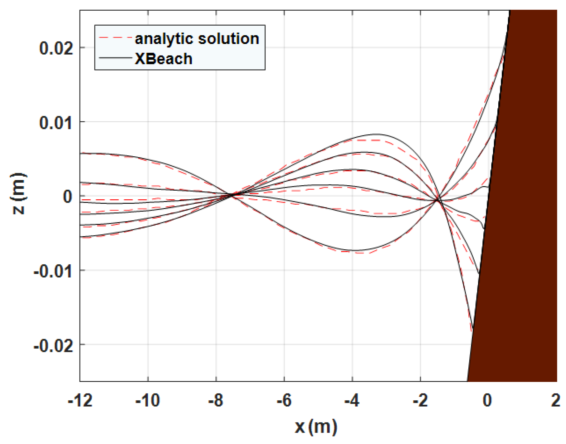
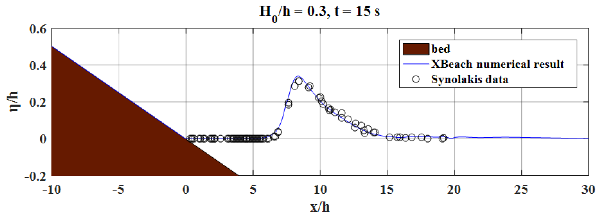
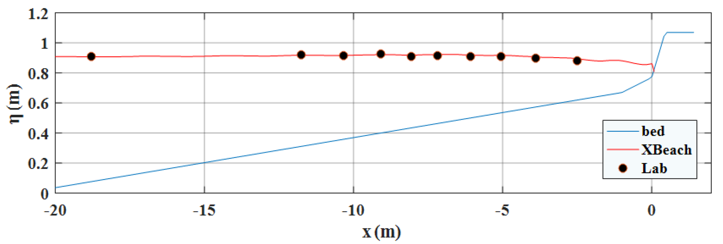
All the numerical experiments presented in this paper were conducted using XBeach [20], which solves the following set of depth-averaged continuity equation

$$\frac{\partial \eta }{\partial t}+\frac{\partial \left(HU\right)}{\partial x}+\frac{\partial \left(HV\right)}{\partial y}=0$$

(1)

and the momentum equations

$$\begin{array}{c}\frac{\partial \left(HU\right)}{\partial t}+\frac{\partial }{\partial x}\left(H{U}^2+\frac{1}{2}g{H}^2+H\overline{p}-\frac{1}{\rho }H{\overline{\tau }}_{xx}\right)+\frac{\partial }{\partial y}\left(HUV-\frac{1}{\rho }H{\overline{\tau }}_{xy}\right)\hfill \\ \hfill =gH\frac{\partial h}{\partial x}-p\frac{\partial h}{\partial x}+\frac{F_{v,x}}{\rho }+\frac{{\tau }_{bx}}{\rho },\end{array}$$

(2)

$$\begin{array}{c}\frac{\partial \left(HV\right)}{\partial t}+\frac{\partial }{\partial x}\left(HVU-\frac{1}{\rho }H{\overline{\tau }}_{yx}\right)+\frac{\partial }{\partial y}\left(H{V}^2+\frac{1}{2}g{H}^2+H\overline{p}-\frac{1}{\rho }H{\overline{\tau }}_{yy}\right)\hfill \\ \hfill =gH\frac{\partial h}{\partial y}-p\frac{\partial h}{\partial y}+\frac{F_{v,y}}{\rho }+\frac{{\tau }_{by}}{\rho },\end{array}$$

(3)

$$\begin{array}{c}\hfill \frac{\partial \left(HW\right)}{\partial t}+\frac{\partial \left(HUW\right)}{\partial x}+\frac{\partial \left(HVW\right)}{\partial y}=-p{|}_{z=-h}^{z=\eta }+\frac{1}{\rho }\frac{\partial \left(H{\overline{\tau }}_{zx}\right)}{\partial x}+\frac{1}{\rho }\frac{\partial \left(H{\overline{\tau }}_{zy}\right)}{\partial y},\end{array}$$

(4)

where $(x,y)$ and z denote the horizontal and vertical directions, respectively, t is time, g the gravitational acceleration, $\rho$ the water density, $\eta$ the free-surface elevation, h the water depth, $H=h+\eta$ the total depth, $(U,V,W)$ the depth-averaged velocity components in $(x,y,z)$ directions, $\tau$ the viscous shear stresses, ${\tau }_b$ the bottom shear stresses modeled by the common quadratic form using, p the dynamic pressure normalized by $\rho$, the overbar denotes the depth-averaged quantities, and finally $F_v$ is the additional force due to the presence of the vegetation. With regard to the boundary conditions, the continuous of normal and tangential stresses are required along the free surface and the kinematic boundary condition is satisfied at the bottom. The model equations are solved by the finite difference method using central difference for the spatial derivatives and the Hansen scheme (the staggered grids in space with explicit scheme on regular time steps) for the coupling between velocity components, $(U,V)$, and free surface elevation, $\eta$. We will not present the detailed numerical discretization or discuss the numerical treatments for specific terms. Interested readers are referred to Smit et al. [21] for details. The main objective here is to investigate the ad-hoc vegetation term, $F_v$, to account for the presence of aquatic vegetation, which results in an additional wave energy dissipation. The analysis will be conducted through a series of numerical experiments and will be presented in Section 3.1. Further application of our new results will also be discussed in Section 3.

2.2. Validation

XBeach has been successfully applied to a study large number of coastal engineering problems such as wave-driven dune erosion [22], gravel beach dynamics [23], dynamic coastal flooding [24], to name a few. However, in order for us to gain a better understanding of the performance of XBeach [20] and its resolution requirement, we briefly carry out some common validations for numerical simulation of wave propagation. We note that the vegetation effect, i.e., the $F_v$ term, has been omitted for the time being. As a first check, we simulate the propagation of a solitary wave on a frictionless flat bottom. Figure 1 shows an example of the comparison between the numerical results and the analytical solution of the solitary wave in a dimensionless manner. In this case, the initial wave nonlinearity is $\epsilon =0.2$, and a fairly dense spatial resolution of 100 grid points per wavelength with Courant number $C=0.1$ are adopted. As can be seen in the figure, the agreement is still satisfactory after a propagation distance of around 30 wavelengths, which suggests the accuracy of the numerical model.

Next, we model the wave runup on a beach and compare the numerical results with the existing analytical solution and experimental data. Both linear progressive waves and solitary waves are examined. Figure 2 shows an exemplary case of our simulations along with the classical analytical solutions by Carrier and Greenspan [25] for a sinusoidal wave propagating on a 1:25 plane beach. Figure 3, on the other hand, demonstrates the comparison with the experiments conducted by Synolakis [26] for a solitary wave of $\epsilon =0.3$ first propagating on a constant depth of 0.1 m and then climbing up a 1:19.85 planer beach. Good agreements are observed for both cases. In Figure 4, we further present the maximum runup heights, R, for solitary waves with nonlinearity from $\epsilon =0.005$ to $\epsilon =0.7$, which covers a wide range of both non-breaking waves and breaking waves. In our simulations, we also turned on the bottom friction with a Chézy type friction coefficient, $C_f=75$. We note that the bottom friction term, i.e., ${\tau }_b$ in the momentum Equations (2) and (3), is mainly to account for the wave breaking. The calculations again are reasonably close to the measurements by Synolakis [26].

Finally, we perform an additional test on the propagation and runup of random waves by reproducing the laboratory tests conducted by Løvås and Tørum [27]. In their experiments, a composite beach with a constant depth region being connected continuously to a 1:30 slope, a 1:10 slope, and finally a steeper 1:1.5 slope was employed, and the wavemaker motion signal was based on the JONSWAP spectrum. Figure 5 shows the realization of one example with peak frequency 2.5 s, significant wave height 0.14 m and constant depth of 0.77 m. Compared to the measured free-surface elevation at several wave gauges, the difference is genuinely acceptable.

All the above suggests that the numerical treatment for the moving boundary and the breaking mechanism perform fairly well. This gives us the confident to perform the numerical experiments on wave-vegetation interaction built upon XBeach [20].

3. Results and Discussion

In this section, we will first discuss the use of a drag force model to account for the additional wave energy dissipation by vegetation. The required drag coefficient will be determined through a series of numerical experiments using XBeach. A new formula for the drag coefficient will be proposed and its applicability will be examined using additional laboratory measurements. Afterward, we will discuss the effect of total width of the vegetation patch, $L_v$, on the wave damping efficiency of the vegetated bed.

3.1. Numerical Experiments for Drag Coefficient

We now proceed to evaluate the effectiveness of using an additional force term, i.e., $F_v$ in the momentum Equations (2) and (3), to model the additional wave dissipation by vegetation. In general, the wave force acting on a small structure can be described by the well-known Morison equation [28], which states that the inline force is obtained by the sum of two force components, namely inertial force and drag force. This parametrized equation requires two empirical hydrodynamic coefficients, the so-called inertia coefficient, $C_M$, and the drag coefficient, $C_D$. Our goal here is therefore to provide an explicit estimation of the coefficients, which is achieved by conducting a series of numerical experiments with the help of the available laboratory measurements in the literature, namely the data collected by Huang et al. [29], Koftis et al. [30], Dubi and Tørum [31], Anderson et al. [32], and Sánchez-González, Sánchez-Rojas and Memos [33]. In other words, we will perform XBeach simulations to mimic the measurements of these five existing experimental studies so that the desired hydrodynamic coefficients can be obtained. The typical laboratory setup in these past studies that we collected is sketched in Figure 6, and the corresponding experimental conditions are listed in

Table 1. Experimental conditions of the laboratory studies used in the present numerical tests on the modeling of wave damping by vegetation.

	Group A ${}^1$	Group B ${}^2$	Group C ${}^3$	Group D ${}^4$	Group E ${}^5$
Model wave ${}^6$	S	J	J	J	J
$H_0$ (m)	0.02, 0.04, 0.05	0.28∼0.35	0.084∼0.187	0.052∼0.193	0.0255∼0.1179
$T_p$ (s)	—	2, 3, 3.5, 4	1.89, 2.21, 2.53, 3.79	1.25, 1.5, 1.75, 2, 2.25	1.25
h (m)	0.15	1.1, 1.3	0.4, 0.6, 0.7, 1	0.305, 0.457, 0.533	0.3, 0.5
Vegetation type ${}^7$	R	F	F	F	F
$h_v$ (m)	0.3	0.55	0.2	0.415	0.1
$D_v$ (m)	0.01	0.01	0.025	0.0064	0.003
$L_v$ (m)	0.545, 1.09, 1.635	9.8	9.3	9.8	9
$N_v$ (# of stem/m${}^2$)	560	180, 360	1200	100, 200, 400	4000
# of cases	7	9	4	32	8

${}^1$ Huang et al. [29]. ${}^2$ Koftis et al. [30]. ${}^3$ Dubi and Tørum [31]. ${}^4$ Anderson et al. [32]. ${}^5$ Sánchez-González, Sánchez-Rojas and Memos [33]. ${}^6$ S: solitary wave; J: JONSWAP spectrum; $H_0$: initial wave height; $T_p$: peak wave period; h: water depth. ${}^7$ R: rigid; F: flexible; $h_v$: steam height; $D_v$: stem diameter; $L_v$: width of the vegetated bed; $N_v$: vegetation density.

. The experiments reported by Huang et al. [29] were conducted in a 32 m long and 0.55 m wide wave flume with 7 wave gauges being adopted to collect free-surface elevation across the model forest. Koftis et al. [30] employed a larger wave flume with 100 m in length and 3 m in width. In addition, 10 resistive wave gauges were used to monitor wave transformation along the model meadow. Measurements reported by Dubi and Tørum [31] was collected by 8 wave gauges in a 33 m long and 1 m wide wave tank. Anderson et al. [32] conducted experiments in two different wave flumes, which were 1.5 m and 3.0 m wide, 63.4 m long, and 1.5 m deep. In their study, water surface oscillations were measured by 18 single wire capacitance-type wave gauges in the 3.0 m flume while 13 gauges were used in the 1.5 m flume. With regard to the experiments by Sánchez-González, Sánchez-Rojas and Memos [33], a relatively wider 46.3 m long and 6.5 m wide wave flume was employed along with 8 gauges equally spaced across the vegetated water. Finally, piston-type wavemakers were all used in these five studies. Overall, 60 cases will be simulated, covering a wide range of wave conditions and the layout of model vegetation. Both submerged and emergent vegetation are considered, with either rigid or flexible plant stems. The density of the vegetated bed ranges from 180 to 4000 stems per meter-square area of the model vegetation. Details of each laboratory experiments can be obtained in the references given in Table 1.

To perform the numerical experiments, we need the expression for $F_v$ appearing in the momentum Equations (2) and (3). We note that if a solid cylinder is considered the relative importance of the inertia term and the drag term in the Morison equation depends on the diameter of the cylinder, D. Dean and Dalrymple [34] suggested that the inertia force dominates when the Keulegan–Carpenter number, $K_C=uT/D$ with u being the water particle velocity and T the wave period, is small. Ozeren, Wren and Wu [35] further showed experimentally that the inertia term becomes negligible when $K_C$ is roughly greater than 20. Reviewing our cases listed in Table 1, we observe from Figure 7 that the corresponding $K_C$ are all greater than 20, suggesting that the drag term dominates. In fact, for the typical wave-vegetation problem $K_C$ is presumably not small since the stem diameter, $D_v$, is usually not too large. Consequently, the additional term used to describe the bulk effect of the vegetation patch on wave propagation can be expressed as

$$F_v=\frac{1}{2}\rho C_D{D}_v{N}_v{h}_v\mathbf{U}\left|\mathbf{U}\right|,$$

(5)

where $N_v$ is the number of plant per meter-square area of the model vegetation, $h_v$ the plant height, and $\mathbf{U}=(U,V)$ the depth-averaged horizontal velocity.

Using (5) to help describe the additional wave damping caused by the presence of vegetation, we are able to simulate numerically the wave-vegetation problem. Figure 8 demonstrates some of our calculations. The wave attenuation is clearly observed, where the wave height can be attenuated as much as 40% across the vegetation patch. By fitting the computed free-surface profiles with the measurements at the available wave gauge, the drag coefficient, $C_D$, has been determined for every case of the overall 60 tests. Collecting all the calibrated $C_D$, we develop an explicit formula for the drag coefficient as

$$C_D=\left[1.0146+{\left(\frac{1.663\times {10}^3}{{\mathrm{Re}}_v}\right)}^{0.7252}\right]{\left(\frac{h_e}{h}\right)}^{1.533},{\mathrm{Re}}_v=\frac{u{D}_v}{\nu },$$

(6)

where $\nu$ is the kinematic viscosity of water, u represents the characteristic water particle velocity and is calculated directly using the incident wave condition [9], $h_e=\min (h_v,h)$. We recall $h=$ water depth, $h_v=$ plant height, and $D_v=$ stem diameter as have been defined previously in (5). The performance of (6) is examined in Figure 9, which plots the predictions by (6) against the numerically calibrated $C_D$. The coefficient of determination is $R^2=0.91$ and the largest derivation is around 25%. In Figure 10 we further examine the sensitivity of $C_D$ by comparing the results obtained by (6) with those carrying 25% difference in the value of $C_D$. In this case, the prediction for $C_D$ works fairly well and even with ±25% difference in $C_D$ the numerical results show less than 10% error in wave height. We believe that the results presented here are reasonable as we adopted a relatively simple drag force model to describe the vegetation effect, i.e., (5) and the experiments considered here indeed cover a wide range of conditions. In Section 3, we will present the application of the numerical model based on the drag force term, (5), with (6) to explicitly pre-determined $C_D$.

3.2. Drag Coefficient Formula

To understand the effectiveness of the drag coefficient Formula (6), we compare our model results with three available laboratory studies in the literature that have not been included in the previous numerical experiments for $C_D$ discussed in Section 3.1.

Table 2. Experimental conditions of the laboratory tests used to examine the effectiveness of the drag coefficient Formula (6).

	Wu ${}^1$	Wu & Cox ${}^2$	WZOW ${}^3$
Model wave ${}^4$	J	J	J
$H_0$ (m)	0.041, 0.033, 0.024, 0.016	0.0342	0.034
$T_p$ (s)	1.6	1.6	1.2
h (m)	0.12	0.12	0.5
Vegetation type ${}^5$	R	R	R, F
$h_v$ (m)	0.14	0.14	0.63, 0.48
$D_v$ (m)	0.005	0.005	0.0094
$L_v$ (m)	1.8	0.9	3.66
$N_v$ (# of stem/m${}^2$)	2100	1618	350, 623, 350
# of cases	4	1	3

${}^1$ Wu [36]. ${}^2$ Wu and Cox [37]. ${}^3$ Wu et al. [12]. ${}^4$ J: JONSWAP spectrum; $H_0$: initial wave height; $T_p$: peak wave period; h: water depth. ${}^5$ R: rigid; F: flexible; $h_v$: steam height; $D_v$: stem diameter; $L_v$: width of the vegetated bed; $N_v$: vegetation density.

summarizes the experimental conditions of these laboratory tests. The comparison between the laboratory measurements and the numerical simulations using (6) for all 8 cases is shown in Figure 11. Visually, the agreement is reasonable, suggesting that the estimation of $C_D$ by the explicit Formula (6) is quite encouraging.

3.3. Width of the Vegetation Patch

In some situations, a single strip of vegetation bed can be cut by the flow and becomes several isolated vegetated patches. Intuitively, this may decrease the wave attenuation by vegetation. To investigate the effect of this type of discontinuity on wave damping, we design a simple numerical experiment by replacing a whole vegetation bed with two smaller patches at both ends and a unvegetated open space in the middle. Our scenario study is presented in Figure 12. The case demonstrated in Figure 11a, which has a unconnected vegetated strip of 1.8 m in width, is used as the baseline to be compared with three designed cases with a central opening of 0.2 m (11%), 0.6 m (33%), and 1.0 m (55%), respectively. Figure 12 shows that, as expected, when the opening is only 0.2 m the wave height at the exit of the whole vegetated bed is barely changed. However, when the open space increases to 55% of the entire vegetated bed, the wave height at the exit increases roughly by 30% (see Figure 12c). As for the case with 33% opening, Figure 12b shows that the exit wave height increases only around 10%, which is nice. This suggests that, as far as the exit wave height is considered, it is unnecessary for the plants to cover the entire width of the designed vegetated strip. In view of the practical engineering design for a green belt protection, this implies that some of the initial tree-planting expenses and the follow-up operation and maintenance costs can potentially be saved.

4. Concluding Remarks

We reported a numerical model based on XBeach to evaluate the effectiveness of wave attenuation by vegetation. The model implemented the non-hydrostatic depth-integrated wave equations with a quadratic drag force term to account for the wave damping by the vegetated bed. The numerically predicted wave height agreed reasonably with the laboratory measurements available in the literature for both emergent vegetation and submerged vegetation. Our simulations showed that the attenuation of wave height at the exit of vegetated bed affected only sightly by the small openings in the middle of the vegetation strip. This suggests the idea of the efficient planning of coastal vegetation planting for the design of such natural-based shore protecting barriers. The present heuristic drag force approach requires an empirically determined drag coefficient, $C_D$. With the help of 60 existing laboratory tests covering various experimental conditions, we successfully developed a simple equation for $C_D$ as a function of Reynolds number through a series of numerical experiments using our model. The new formula for the drag coefficient is attractive since it is easy to use and provides a priori estimation of $C_D$ for the given incident wave conditions and vegetation configurations. Furthermore, it can be applied for waves through either a submerged vegetated bed or surface piercing vegetation. Since the model with the new $C_D$ can reasonably capture the variation of wave height across the vegetated water, which is one of the most pertinent measures of the effectiveness of green belt protection, without resolving small-scale fluid motion surrounding plant stems that requires massive computations, the numerically expedient model has the potential to serve as tool for a scientific assessment of the real-scale engineer design of using such bio-shields for coast protection.

We note that the drag force model that we adopted in this study is a simplistic approach, which provides only an integrated effect of wave damping by vegetation. To make the formula for $C_D$ more robust, we shall consider more explicitly some vegetation properties such as vegetation flexibility and root conditions. Furthermore, our $C_D$ was determined empirically based on measurements obtained in wave tanks of typical size. We expect the formula may still be applicable to large-scale problem since we believe that the experiments we considered covered a wide range of vegetation and wave conditions and the scaling laws have been properly followed in these studies. Of course, the reliability of numerical solutions for engineering-scale problem would require further examination using field data. Finally, all the cases presented here involve only one horizontal dimension (1HD). In principle, the approach introduced here can be applied to 2HD problems, which will be more useful for the practical engineering application. However, to formulate the corresponding equation for $C_D$ a considerable amount of additional experimental data is required. Comparing to the existing of a vast literature on the wave tank experiments, available 2HD laboratory studies on wave-vegetation is still limited. We remark that Liu et al. [17] reported a large-scale wave basin experiment on plane waves through a circular forest. Of course, the two-dimensional scatting is very different from the 1HD problem presented in this paper. We are desired to learn more 2HD experiments on wave-vegetation.

References

1. Danielsen, F.; Sørensen, M.K.; Olwig, M.F.; Selvam, V.; Parish, F.; Burgess, N.D.; Hiraishi, T.; Karunagaran, V.M.; Rasmussen, M.S.; Hansen, L.B.; et al. The Asian Tsunami: A protective role for coastal vegetation. Science 2005, 310, 643. [Google Scholar] [CrossRef] [PubMed] [Green Version]
2. Ranghieri, F.; Ishiwatari, M. Learning from Megadisasters: Lessons from the Great East Japan Earthquake; World Bank: Washington, DC, USA, 2014. [Google Scholar]
3. Das, S.; Vincent, J.R. Mangroves protected villages and reduced death toll during Indian super cyclone. Proc. Natl. Acad. Sci. USA 2009, 106, 7357–7360. [Google Scholar] [CrossRef] [PubMed] [Green Version]
4. Costanza, R.; Peŕez-Maqueo, O.; Martinez, M.L.; Sutton, P.; Anderson, S.J.; Mulder, K. The value of coastal wetlands for hurricane protection. Ambio 2008, 37, 241–248. [Google Scholar] [CrossRef]
5. Massel, S.R.; Furukawa, K.; Brinkman, R.M. Surface wave propagation in mangrove forests. Fluid Dyn. Res. 1999, 24, 219–249. [Google Scholar] [CrossRef]
6. Möller, I.; Spencer, T.; French, J.R.; Leggett, D.J.; Dixon, M. Wave transformation over salt marshes: A field and numerical modelling study from North Norfolk, England. Estuar. Coast. Shelf Sci. 1999, 49, 411–426. [Google Scholar] [CrossRef]
7. Luhar, M.; Infantes, E.; Nepf, H. Seagrass blade motion under waves and its impact on wave decay. J. Geophys. Res. Oceans 2017, 122, 3736–3752. [Google Scholar] [CrossRef] [Green Version]
8. Cavallaro, L.; Viviano, A.; Paratore, G.; Foti, E. Experiments on surface waves interacting with flexible aquatic vegetation. Ocean Sci. J. 2018, 53, 461–474. [Google Scholar] [CrossRef] [Green Version]
9. Lei, J.; Nepf, H. Wave damping by flexible vegetation: Connecting individual blade dynamics to the meadow scale. Coast. Eng. 2019, 147, 138–148. [Google Scholar] [CrossRef]
10. Tang, J.; Causon, D.; Mingham, C.; Qian, L. Numerical study of vegetation damping effects on solitary wave run-up using the nonlinear shallow water equations. Coast. Eng. 2013, 75, 21–28. [Google Scholar] [CrossRef]
11. Augustin, L.N.; Irish, J.L.; Lynett, P. Laboratory and numerical studies of wave damping by emergent and near-emergent wetland vegetation. Coast. Eng. 2009, 56, 332–340. [Google Scholar] [CrossRef]
12. Wu, W.; Zhang, M.; Ozeren, Y. Analysis of Vegetation Effect on Waves Using a Vertical 2D RANS Model. J. Coast. Res. 2013, 29, 383–397. [Google Scholar] [CrossRef]
13. Maza, M.; Lara, J.L.; Losada, I.J. A coupled model of submerged vegetation under oscillatory flow using Navier–Stokes equations. Coast. Eng. 2013, 80, 16–34. [Google Scholar] [CrossRef]
14. Kim, S.J.; Stoesser, T. Closure modeling and direct simulation of vegetation drag in flow through emergent vegetation. Water Resour. Res. 2011, 47, W10511. [Google Scholar] [CrossRef]
15. Chakrabarti, A.; Chen, Q.; Smith, H.D.; Liu, D. Large eddy simulation of unidirectional and wave flows through vegetation. J. Eng. Mech. 2016, 142, 04016048. [Google Scholar] [CrossRef] [Green Version]
16. Mei, C.C.; Chan, I.-C.; Liu, P.L.-F.; Huang, Z.; Zhang, W. Long waves through emergent coastal vegetation. J. Fluid Mech. 2011, 687, 461–491. [Google Scholar] [CrossRef]
17. Liu, P.L.-F.; Chang, C.-W.; Mei, C.C.; Lomonaco, P.; Martin, F.L.; Maza, M. Periodic water waves through an aquatic forest. Coast. Eng. 2015, 96, 100–117. [Google Scholar] [CrossRef]
18. Wei, G.; Kirby, J.T.; Grilli, S.T.; Subramanya, R. A fully nonlinear Boussinesq model for surface waves. Part I. Highly nonlinear unsteady waves. J. Fluid Mech. 1995, 294, 71–92. [Google Scholar] [CrossRef]
19. Lynett, P.; Wu, T.-R.; Liu, P.L.-F. Modeling wave runup with depth-integrated equations. Coast. Eng. 2002, 46, 89–107. [Google Scholar] [CrossRef]
20. Roelvink, D.; Reniers, A.; van Dongeren, A.; van Thiel de Vries, J.; McCall, R.; Lescinski, J. Modelling storm impacts on beaches, dunes and barrier islands. Coast. Eng. 2009, 56, 1133–1152. [Google Scholar] [CrossRef]
21. Smit, P.; Stelling, G.; Roelvink, D.; van Thiel de Vries, J.; McCall, R.; van Dongeren, A.; Zwinkels, C.; Jacobs, R. XBeach: Non-Hydrostatic Model; Delft University of Technology and Deltares: Delft, The Netherlands, 2010. [Google Scholar]
22. Berard, N.A.; Mulligan, R.P.; da Silva, A.M.F.; Dibajnia, M. Evaluation of XBeach performance for the erosion of a laboratory sand dune. Coast. Eng. 2017, 125, 70–80. [Google Scholar] [CrossRef]
23. Jamal, M.H.; Simmonds, D.J.; Magar, V. Modelling gravel beach dynamics with XBeach. Coast. Eng. 2014, 89, 20–29. [Google Scholar] [CrossRef]
24. Gallien, T.W. Validated coastal flood modeling at Imperial Beach, California: Comparing total water level, empirical and numerical overtopping methodologies. Coast. Eng. 2016, 111, 95–104. [Google Scholar] [CrossRef] [Green Version]
25. Carrier, G.F.; Greenspan, H.P. Water waves of finite amplitude on a sloping beach. J. Fluid Mech. 1958, 4, 97–109. [Google Scholar] [CrossRef]
26. Synolakis, C.E. The runup of solitary waves. J. Fluid Mech. 1987, 185, 523–545. [Google Scholar] [CrossRef]
27. Løvås, S.M.; Tørum, A. Effect of the kelp Laminaria hyperborea upon sand dune erosion and water particle velocities. Coast. Eng. 2001, 44, 37–63. [Google Scholar] [CrossRef]
28. Morison, J.; Johnson, J.; Schaaf, S. The force exerted by surface waves on piles. J. Pet. Technol. 1950, 2, 149–154. [Google Scholar] [CrossRef]
29. Huang, Z.; Yao, Y.; Sim, S.Y.; Yao, Y. Interaction of solitary waves with emergent, rigid vegetation. Ocean Eng. 2011, 38, 1080–1088. [Google Scholar] [CrossRef]
30. Koftis, T.; Prinos, P.; Stratigaki, V. Wave damping over artificial Posidonia oceanica meadow: A large-scale experimental study. Coast. Eng. 2013, 73, 71–83. [Google Scholar] [CrossRef]
31. Dubi, A.; Tørum, A. Wave energy dissipation in kelp vegetation. Coast. Eng. Proc. 1996, 2, 2626–2639. [Google Scholar]
32. Anderson, M.E.; Smith, J.M.; Bryant, D.B.; McComas, R.G.W. Laboratory Studies of Wave Attenuation through Artificial and Real Vegetation; ERDC TR-13-11; U.S. Army Engineer Research and Development Center: Vicksburg, MS, USA, 2013. [Google Scholar]
33. Sánchez-González, J.F.; Sánchez-Rojas, V.; Memos, C.D. Wave attenuation due to Posidonia oceanica meadows. J. Hydraul. Res. 2011, 49, 503–514. [Google Scholar] [CrossRef]
34. Dean, R.G.; Dalrymple, R.A. Water Wave Mechanics for Engineers and Scientists; World Scientific Publishing Company: Singapore, 1991. [Google Scholar]
35. Ozeren, Y.; Wren, D.; Wu, W. Experimental investigation of wave attenuation through model and live vegetation. J. Waterw. Port. Coast. 2013, 140, 04014019. [Google Scholar] [CrossRef]
36. Wu, W.-C. Effects of Wave Nonlinearity and Vertical Variation of Vegetation Density on Wave Attenuation. Ph.D. Dissertation, Oregon State University, Corvallis, OR, USA, 2015. [Google Scholar]
37. Wu, W.-C.; Cox, D.T. Effects of vertical variation in vegetation density on wave attenuation. J. Waterw. Port. Coast. 2015, 142, 04015020. [Google Scholar] [CrossRef]
Figure 1. Propagation of a solitary wave on a frictionless flat bottom: snapshots of free-surface profile at various time stamps. Solid: numerical results by XBeach [20]. Dashed: analytical formulation for solitary wave. H 0 and h denote the initial wave height and the water depth, respectively, and L is the wavelength. The initial wave nonlinearity is ε = H 0 / h = 0.2 and the spatial resolution is 100 grids per wavelength.
Water 12 02513 g001
Figure 2. Runup of a liner progress wave on a plane beach with a slope of 1:25: snapshots of free-surface profile at various time stamps. Solid: numerical results by XBeach [20]. Dashed: analytical predictions by Carrier and Greenspan [25]. The incident wave has a period of 10 s and 0.006 m in wave height.
Water 12 02513 g002
Figure 3. Runup of a solitary wave on a beach: snapshot of free-surface profile at t = 15 s. Line: numerical results by XBeach [20]. Symbol: experimental data by Synolakis [26]. The initial wave nonlinearity is 0.3, the constant depth is 0.1 m, and the beach slope is 1:19.85.
Water 12 02513 g003
Figure 4. Dimensionless maximum runup height ( R / h ) of a solitary wave on a 1:19.85 beach as a function of the initial wave nonlinearity ( H 0 / h ) . Symbol: experimental data by Synolakis [26]. Dashed: numerical results by XBeach [20] with zero bottom friction. Solid: XBeach results with additional bottom friction using a Chézy coefficient C f = 75 .
Water 12 02513 g004
Figure 5. Free-surface profile of a random wave generated with JONSWAP spectrum propagating on a composite beach. Symbol: laboratory data by Løvås and Tørum [27]. Line: numerical results by XBeach [20]. In this case, the peak frequency of the incident wave is 2.5 s, the significant wave height is 0.14 m, and the constant depth is 0.77 m. The part of the composite beach shown here has a slope of 1:30, 1:10, and 1:1.5 (from left to right).
Water 12 02513 g005
Figure 6. Typical experimental setup for the laboratory study on wave through a vegetated water with either submerged or emergent vegetation. H 0 : initial wave height; h: constant water depth; h v : vegetation steam height; D v : stem diameter; L v : width of the vegetated bed. A typical wave absorbing beach is usually installed at the end of the wave tank.
Water 12 02513 g006
Figure 7. Keulegan–Carpenter number, K C , for all 60 experimental cases summarized in Table 1 with the dashed line indicating the threshold value K C = 20 . Group A: Huang et al. [29]. Group B: Koftis et al. [30]. Group C: Dubi and Tørum [31]. Group D: Anderson et al. [32]. Group E: Sánchez-González, Sánchez-Rojas and Memos [33]. See Table 1 for the experimental conditions of each group.
Water 12 02513 g007
Figure 8. Examples of the normalized wave height across the model vegetation for the experiments listed in Table 1. (a) Huang et al. [29]. (b) Koftis et al. [30]. (c) Anderson et al. [32]. (d) Dubi and Tørum [31]. (e) Sánchez-González, Sánchez-Rojas and Memos [33]. Symbol: measurements. Line: numerical results. Vertical bars at the bottom are plotted to indicate the location of the vegetation patch and do not reflect the real stem heights.
Water 12 02513 g008
Figure 9. The predicted drag coefficient, C D , by the explicit Formula (6) vs. the numerically calibrated C D for all 60 cases. The coefficient of determination is R 2 = 0.91 . Dashed lines indicate the 25% bounds. See Table 1 for the conditions of each Group.
Water 12 02513 g009
Figure 10. Example of the sensitivity test on the drag coefficient, C D . Symbol: laboratory data. Solid: simulation using C D calculated by (6). Dashed and dotted: simulations with ±25% difference in the value of C D . The maximum differences in wave height for C D = 1.478 and 2.463 are 9.4% and 7.1%, respectively.
Water 12 02513 g010
Figure 11. Normalized wave height across the model vegetation for all 8 cases listed in Table 2. (a) Case 1 of Wu [36]. (b) Wu and Cox [37]. (c) Case 2 of Wu [36]. (d) Case 1 of Wu et al. [12]. (e) Case 3 of Wu [36]. (f) Case 2 of Wu et al. [12]. (g) Case 4 of Wu [36]. (h) Case 3 of Wu et al. [12]. Symbol: measurements. Line: numerical results with the of CD calculated explicitly by (6). Vertical bars at the bottom are plotted to indicate the location of the vegetation patch and do not reflect the real stem heights. See Table 2 for the detailed experimental conditions.
Water 12 02513 g011
Figure 12. Normalized wave height across the model vegetation with different width of unvegetated open space in the middle of the vegetated bed. (a) 0.2 m open space. (b) 0.6 m open space. (c) 1.0 m open space. Symbols in all panels show the same set of laboratory measurements employing a whole 1.8 m wide vegetation bed, which is the identical case illustrated in Figure 11a. Line: numerical results with the of CD calculated explicitly by (6). Vertical bars at the bottom are plotted to indicate the location of the vegetation patch and do not reflect the real stem heights.
Water 12 02513 g012