Abstract
Fluvial geomorphic approaches for reclamation landform design have been applied since 2000, mostly in mined lands, as an alternative to conventional landform design methods. Those approaches aim to reconstruct mature landforms and drainage networks that would develop within a natural catchment, after thousands of years of work performed by geomorphic processes. Some fluvial geomorphic design methods take specific measurements from natural and stable reference areas for initial input values for reclamation design. Valid reference areas can be difficult to find, can be in highly anthropized environments, or may be difficult to access. This paper evaluates the use of remote sensing tools to measure morphometric parameters in upper sections of agricultural land catchments considered for use as reference areas. The ridge to head of channel distance (Xrh) was the parameter of interest. We used land surface profiles developed from LiDAR (Laser Imaging Detection and Ranging) data and planimetric measurements from orthoimages to estimate Xrh. The results obtained by the two methods were encouraging but showed a significant difference. Ground truthing showed that ploughing obliterated between 19.5 and 22.4 m (on average) of the headwater section of first-order channels, reducing the channel length by 15.1 to 32.4%. Using a greater Xrh value than appropriate for near steady-state conditions as a design input for a geomorphic reclamation project would be expected to result in active erosion processes in the constructed reclamation to regain their missing channel length. We recognize the advantages and limitations of remote sensing methods for measuring the morphometric parameters of the landform relief design inputs. We show how these tools may be used to help select and prioritize reference areas, and warn about the use of disturbed landscapes as reference areas to assure the geomorphic stability of the constructed reclamation designs.
1. Introduction
The mining industry is an essential activity in order to support modern living. However, it is often despised because of the significant impact it can have on the land. These concerns are usually reflected by environmental laws [1,2,3,4]. Where mining activity coincides with ecologically sensitive landscapes, it is necessary to ensure the physical and chemical stability of mining wastes during operation and after its closure [1,2,3,4].
In order to comply with those regulations and conditioning factors, mining companies need to design closure plans that take into account the restoration (or reclamation, the term we use in this paper) of the disturbed land. Traditional topographic reconstruction approaches, such as outslope/berm systems, rectilinear slopes, and drainage ditches, aim primarily to maximize the material storage volume with a minimum footprint, convey water away from the disturbed areas, and attain geotechnical stability for the unconsolidated spoils [5,6]. River relocation is also a common practice in mining projects [7]. However, during the last few decades, studies on mine waste erosion have demonstrated that these conventional reclamation practices do not guarantee the long-term stability of the mine wastes and are not self-sustainable [8,9]. Although geotechnically stable, reclamation landforms are usually constructed with little thought about geomorphic principles [10]. In nature, rivers and streams flow downhill, not across slopes, as do the drainage ditches of outslope/berm systems. When a high-intensity storm occurs, conventional drainage ditches fill up, causing water to overflow and erode the mine wastes in an attempt to re-establish the natural drainage density altered by the mining activity. Because of that, the graded landforms usually end up with severe slope erosion that requires maintenance, increasing the cost of the total mine operation, becoming a potential environmental hazard, and possibly delaying the reclamation liability bond release. These problems, and community objections to large monolithic dump structures, have also made it difficult to obtain permits to operate if proposing the traditional landform design methods.
The introduction of geomorphic principles in mine reclamation was not a common regulatory requirement until the late 1970 and early 1980s. The US SMCRA (Surface Mining Control and Reclamation Act) [11] is a pioneer in this regard, describing the need for reclaimed land to complement the drainage pattern of the surrounding terrain. It actually introduced a “catchment approach” in mine reclamation—outlining it as the fundamental unit for planning mine reclamation and guaranteeing hydrological connectivity. This approach was explicitly expressed later by Stiller et al. [12], who asserted that planning for the long-term stability of reclaimed surface mines meant incorporating drainage networks that would integrate into the surrounding landscape. This implies a paradigm shift from the conventional land grading methods. Instead of building linear slopes and artificial drainage that diverts water away from the waste dumps and other disturbed areas with little consideration of proper hydrologic connectivity and function, the catchment approach’s goal is to recreate complex landforms with a functioning drainage pattern similar to those developed on local, mature landscapes.
The underlying geomorphic and fluvial principles introduced by the US SMCRA were the foundation for using modern topographic reconstruction methodologies, such as the GeoFluvTM reclamation method [13,14,15]. GeoFluv is a fluvial-geomorphic land reclamation method that is able to reproduce the complexity of landforms and drainage networks that would develop within a natural, stable catchment. Natural Regrade is a commercialized software [16] that aids the user to efficiently make GeoFluv designs in a CAD (Computer-Aided Design) environment. The method essentially helps the designer approximate steady-state reclamation landforms that would develop on the specific materials, climate, vegetation, and physiographic conditions of the site after thousands of years of work performed by the geomorphic processes. Several morphometric parameters of the landform relief and drainage network must be properly measured and used as design inputs to ensure that the designed landforms function as open, process-response systems with a stable, steady-state configuration. The same fluvial geomorphic processes can occur globally producing similar landforms, but the magnitude of these parameters changes in response to the local conditions; this is why the accurate measurement of localized input values is important to making a site-specific design that will provide the desired, natural hydrologic landform functions for a specified project. The definition of those parameters is not arbitrary, but need to be measured from natural, near steady-state landforms developed on similar earth materials with similar climate and vegetation as the reclamation project. Those landforms are referred to as reference areas and they provide initial input values for the GeoFluv reclamation design. In some areas of the world, satisfactory reference areas can be found readily within a few kilometers around the disturbed mining landscape, but in other areas it can be more difficult because of the effects of centuries of human land disturbances or poor road access. Significant developments in remote sensing technology over the last two decades have led some users of the GeoFluv method to consider if these tools can be used to collect the geomorphic input values without having to visit the reference areas.
The objective of this study is to evaluate the use of remote sensing tools to measure a morphometric parameter from a possible reference area. The ridge to head of channel distance (Xrh) was the parameter of interest. This morphometric parameter can be defined as the convex slope draining to the head of a channel, measured from the head of the channel along the flow line to the divide of the catchment. In this paper, we used both land surface profiles developed from LiDAR (Laser Imaging Detection and Ranging) data and planimetric measurements from orthoimages to estimate and compare the value of Xrh in three catchments affected by the agricultural activity. We will refer to the results obtained by these methods as apparent Xrh (for the orthoimage estimates) and LiDAR convex slope length (for the LiDAR data estimates). In a natural, near steady-state catchment, the LiDAR convex slope length should be equivalent to the apparent Xrh, as they are effectively measuring the same planimetric distance in a channel’s longitudinal profile. Significant deviations between the values obtained using the two measurement methods could indicate signs of instability or disturbances in the channel’s longitudinal profile, or point to inaccuracy in one or both methods.
In this study, we do not intend to do an exhaustive review of the GeoFluv method nor its potentialities in modern geomorphic land reclamation. Here, we will focus in the assessment of the uses and applications of some remote sensing tools to collect input parameters for geomorphic reclamation designs. However, a basic overview of the GeoFluv method will be presented in the methodology so the readers can have an overall idea of the basic notions behind this fluvial-geomorphic reclamation method and understand why measuring accurate input values is important.
With this research, we hope to contribute to the success of future reclamation projects that could make use of the GeoFluv method or other fluvial-geomorphic land reclamation approaches not only in the study area, but also in other regions of the world.
2. Study Area
The three catchments selected for this study are located in the south-eastern margin of the Iberian Pyrite Belt, IPB (southwest Spain), a prolific mining area with more than 150 hm3 total volume of derelict mine wastes affected by water runoff, the leaching of potential toxic elements, and wind erosion that can cause serious environmental damage [17,18]. The IPB, probably the largest known volcanogenic massive sulfide (VMS) ore province in the world, extends from the city of Seville (southwest Spain) to the Portuguese coast, and is approximately 230 km long and 40 km wide [17,18,19] (Figure 1). Its south-eastern margin comprises part of the Guadalquivir Valley, a sedimentary basin composed mostly by Neogene–Quaternary detrital materials (Figure 2) dominated by agricultural land use activity. The selection of this particular area as the study zone has been prompted by the fact that, since 2018, several metallic mines in the IPB are either applying or considering the application of a GeoFluv-based geomorphic reclamation approach. Some examples are the Tharsis, Aguas Teñidas, and Cobre Las Cruces mines in Spain, and the Lousal Mine in Portugal (Figure 1). We used agricultural land catchments in this area to test the use of remote sensing tools to measure the parameter at possible reference areas.
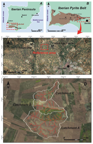
Figure 1.
(A) Location of the Iberian Pyrite Belt (IPB) in the Iberian Peninsula; (B) the IPB and some of its most outstanding metallic mines. The study area is located 18.5 km northwest of Seville (Spain), in the south-eastern margin of the IPB. (C,D) Detailed view of the study area and catchments A, B, and C selected for this study.
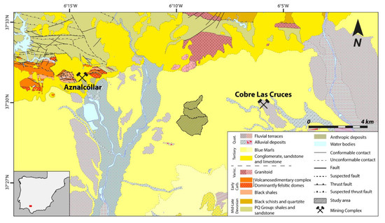
Figure 2.
Study area and geological map of the northern section of the Guadalquivir basin (adapted from IGME, Instituto Geológico y Minero de España, 2008 [20]).
3. Materials and Methods
3.1. The GeoFluv Method
GeoFluvTM is the trademark name for a patented landform design method. It uses algorithms based on fluvial and geomorphic principles to design reclamation landforms that would naturally develop after thousands of years of work performed by geomorphic processes for the specific materials, climate, vegetation, and physiographic conditions at the disturbed site. Natural Regrade is its associated commercialized software that aids the user to make efficient GeoFluv designs in a CAD format [16]. The GeoFluv method is consistent with the “catchment approach”, first sketched out in the US SMCRA [11] and made explicit by Stiller et al. [12], which considers the catchment as the basic planning unit for mine reclamation.
The GeoFluv method began to be applied to large coal mines in New Mexico (United States) in the late 1990s and early 2000s. Since then, it has been successfully applied in numerous mine reclamation projects around the United States [21], Spain [22,23], Australia [24,25], and South America [21]. Its combined use with landscape evolution models (such as SIBERIA) [26] has also been assessed in order to obtain optimal mine rehabilitation outcomes in terms of erosional stability. The method’s ability to provide erosional stability comparable to undisturbed, natural land in the project areas has been quantified by sediment yield research [23,27].
A GeoFluv design uses several input values taken from a suitable, natural reference area for the reclamation design. Here, the word “suitable” refers to geomorphically steady-state landforms (having attained a “mature” fluvial geomorphic state) developed with similar earth materials, climate, and vegetation as the disturbed mine area.
Natural landscapes generally do not maintain a perfect steady state—i.e., in which zero erosion occurs—for more than a very brief period (in the order of weeks, months, a few years at most), as a landform is constantly adjusting to changes in its balance among erosional forces and resistances by geomorphic processes. However, the rates at which the geomorphic processes operate may decrease as they reach a dynamic equilibrium, when no on-site or off-site environmental degradation beyond acceptable natural rates occur [10]. If the input values for the reclamation design are measured from a reference area that is far from reaching a dynamic equilibrium and is eroding at an accelerated rate, then geomorphic processes in the reclamation landscape designed using those inputs will predictably operate at similar rates, with the accelerated erosion and degradation of the reclamation landform.
Conversely, if the reference area is near its steady-state configuration, the designed reclamation landform will experience fewer modifications by geomorphic processes after construction. This property of the fluvial geomorphic reclamation landform offers lower costs because of its long-term stability and self-maintaining performance [28,29,30]. This is why it is important to correctly measure the geomorphic design input values.
The GeoFluv method is applicable for relatively minor to extreme land disturbances to restore steady-state geomorphic conditions. Livestock trampling streambanks is an example of a relatively minor disturbance and a large surface mine is an example of a more extreme disturbance. The GeoFluv method can be used to practically return minor disturbances to their pre-disturbance morphology and function. It may be impractical to return major disturbances to their pre-disturbance morphology, but we can design a different morphology that is appropriate for the post-disturbance land and that will provide the hydrologic functions that support a steady-state landform for the reclamation base. For example, at the end of ore extraction a large surface mine may have made a great pile of waste rock and a large pit, features that were not part of the pre-mine landscape, but through geomorphic-based reclamation they can become part of a new, hydrologically functional reclamation landscape—such as a hill with ephemeral stream channels and a connected pond or lake, for example—that is consistent with local geomorphic processes.
3.2. Measurement of the Ridge to Head of Channel Distance (Xrh)
During October 2019, we conducted field work on agricultural areas near the city of Seville (southwest Spain) (Figure 3). We located catchments whose landforms were well-developed and clearly visible, as can be seen in Figure 4. The tilled, marl-derived soil in the fields was an earth material similar to the broken overburden of the local mine wastes. The catchments were in a similar climatic zone, and the crops would be similar to the post-reclamation vegetation, so the site met the basic reference area criteria. We used these sites to test the remote sensing tools’ applicability for measuring an input parameter from these possible reference areas for a geomorphic reclamation project.
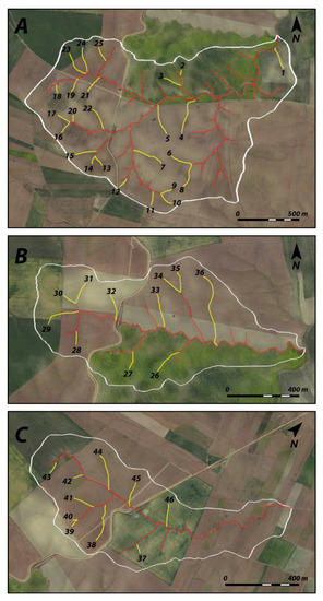
Figure 3.
Selected catchments within agricultural areas located 18.5 km northwest of Seville; (A–C) catchments A, B, and C, respectively. The measured 46 first-order channels are represented in yellow.
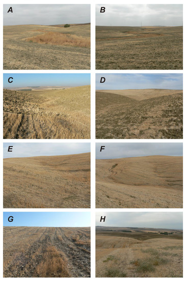
Figure 4.
Field pictures of the studied areas. (A,B) View of the low section of catchment A and B, respectively. (C,D) Views of the mid-section of catchment A. (E,F) Headwater reaches in catchment A. (G) Upstream view from the head of the channel to the water divide (channel 44, catchment C). (H) Downstream view from the water divide of catchment A.
Three small catchments (A, B, and C in Figure 3) were selected 18.5 km northwest of Seville (Figure 3 and Figure 4). The three catchments are developed in late Neogene marls and Quaternary detritic materials of the Guadalquivir fluvial basin, similar to those that form the mine spoils of some of the IPB mines. The surface areas for catchments A, B, and C are 1.98, 0.75, and 0.56 km2, respectively, and support ephemeral streams (discharge only during runoff-generating storm events). Drainage density values for catchments A, B, and C are 4.57, 5.54, and 5.79 km/km2, respectively (Table 1). Forty-six first-order ephemeral channels were selected over the three catchments to measure the ridge to head of channel distance (Xrh) using remote sensing tools. First-order channels without a clearly visible channel head (the point at which a defined channel bed begins) were not selected for this study, as they would introduce uncertainty to the results.

Table 1.
Values of the total channel length, catchment area, and drainage density for catchments A, B, and C.
The ridge to head of channel distance (Xrh) is one of several input values that the GeoFluv method uses to design the reclamation landscape. It is the space between a water divide and the start (head) of the first-order channels, measured along the flow line (Figure 5). This morphometric parameter has key importance, as it reflects the amount of headward erosion a channel has undergone on a slope until it reached a steady state.
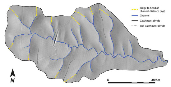
Figure 5.
Schematic view of the ridge to head of channel distance (Xrh, represented with yellow-dashed lines) measured in catchment B. Channels appear represented in blue. The ridge to head of channel distance (Xrh) can be defined as the distance measured from the head of the channel along the flow line to the divide of the catchment.
A similar parameter to the ridge to head of channel distance was first reported by Horton [31]. Horton observed that, for a slope to start eroding, the available eroding force must exceed the resistance of the soil to erosion. As the eroding force increases downslope from the water divide, there will be a certain point on the slope where this force becomes equal to the resistance of the soil. Horton called this the critical distance, Xc. If this point is considered the starting point of concentrated water erosion, no rill or gully erosion should occur from the water divide around the valley until that critical distance downslope is reached, and therefore a “belt of no erosion”, as defined by Horton [31], will develop. We have observed that this behavior is consistent around the catchment divide, with slight variations in Xc, except that the channel forms along one line where the resisting forces are lower and/or the erosive forces are greater than elsewhere around the catchment. For example, because a first-order catchment is relatively small, its earth material (providing resisting forces) is often relatively homogenous, so channel development occurs at the point in the catchment that has a greater upslope area to collect runoff, or has a steeper slope, or that has a combination of these factors (providing erosive forces). The convex slope length is shorter along this line, which we define as the ridge to head of channel distance, Xrh, as compared to the rest of the catchment.
The evolution of the channel profile is conditioned by erosional processes in ephemeral catchments developed in unconsolidated materials with no structural controls. In the upper sections of those catchments, surficial water will run through a sheet flow regime until it reaches a point where the water flow concentrates and has enough energy to start eroding the land surface. From this point downward, water erosion will change the form of the slope from a convex shape to a predominantly concave profile that will continue to the end (mouth) of the channel [32]. If given enough time, geomorphic and erosion processes will lead to the development of a clear convex-to-concave inflection point that is visible on the slope profile and that defines the start (head) of the ephemeral channel. The section of the slope measured along the flow line from this point up to the top of the catchment will then have a convex shape.
This means that, in approximate steady-state catchments developed on unconsolidated materials, Xrh should be very similar for all channels and, by definition, equivalent to the length of the upper convex section of the channels’ longitudinal profile. If those values noticeably differ, it could evidence that the catchment is still adjusting into a steady-state configuration or that it has been disturbed after reaching a steady-state stage. It could also indicate that the site earth materials are not homogenous, unconsolidated materials, but that underlying consolidated rock formations are resisting erosion and the site is not an optimal reference area. This can be recognized in the field—for example, as a ‘”headcut”, where the upper end of the channel abruptly terminates as a vertical wall in the convex slope in unconsolidated material; or a vertical wall of resistant consolidated rock; or, less frequently, as sediment aggraded on the slope at the head of the channel. When these conditions are present, using input parameters collected from those catchments in a geomorphic reclamation project would not be advised.
We estimated and compared the ridge to head of channel distance (Xrh) and the LiDAR convex slope length in the 46 first-order channels. Convex slope lengths may vary at different positions within a catchment. Because channels form where the erosional forces exceed the resisting forces by the greatest factor, the upper convex profile of the slope is expected to be shorter there than elsewhere in a given catchment. In this paper, we only assess the length of the upper convex section of the 46 channels’ longitudinal profile, measured from the divide of the catchments in the direction towards the head of the channel along the flow line. We will not discuss the convex slope lengths in other areas of the catchment, such as the valley walls.
Measurements of the ridge to head of channel distance (Xrh) were performed using GIS processing software (QGIS). High-precision LiDAR point cloud data (0.5 points/m2 density; accuracy and precision of RMSEz ≤ 0.20 m) was acquired from the CNIG (Geographic Information National Center, Government of Spain [33]). The LiDAR data used in this study were captured in 2014, the most recent LiDAR survey available for the study area. We used these data to create a Digital Elevation Model (DEM) of the study zone. A 2 m cell size was chosen in order to ensure that each cell of the DEM had at least one individual x, y, and z value. The DEM was then introduced in the GIS processing software and superimposed with orthoimages of the study zone acquired from the PNOA (Aerial Orthophotography National Plan, Government of Spain [34]). The general technical specifications of the photogrammetric survey are a GSD (Ground Sample Distance, resolution of the image) of 0.45 m/pixel, and RMSEx,y ≤ 1 m [34]. The orthoimages used in this study were captured in 2016.
Ideally, the LiDAR data and orthoimages should be captured during the same year to allow a better comparison of the results obtained from the two methodologies. If that is not possible, the closest data available in time must be used. In our study zone, no orthoimages were available for 2014. The next photogrammetric survey available dated from 2016. Therefore, the orthoimages captured in 2016 were used to minimize as much as possible the time difference between the LiDAR and the photogrammetric surveys. When analyzing the results obtained using the two methodologies, the two-year difference between the LiDAR data and the orthoimages must be taken into account, as deviations between results may be due to changes in the channel morphometry that occurred during that time.
Using the orthoimages as a visual reference, a shapefile containing the planimetric view of the channels’ flow lines (from the channel mouth to the top of the catchment) was created. Finally, the shapefile was combined with the DEM, using the terrain profile tool in QGIS, to obtain the longitudinal profile for each of the 46 channels.
The apparent Xrh (planimetric distance measured with orthoimages) was measured from the highest elevation point of the profile (either the external divide of the catchment or an internal divide) to the visible start (head) of the channel, as seen in the orthoimages. Visible changes in vegetation or clear channel incisions on the slope were used as criteria to establish the head of the channel. This measurement relies heavily on the resolution of the orthoimages and the absence of potential visual obstacles that could obscure the identification of the channels’ head, such as dense vegetation. Therefore, it is best used in areas with low or scarce vegetation cover and available high-resolution photogrammetric surveys. The LiDAR convex slope length was estimated by measuring the distance from the highest point of the slope profile to the convex-to-concave inflection point in each of the 46 channels’ longitudinal profile (Figure 6). Similarly to the orthoimages, the results obtained using this method are expected to be more accurate as the precision and point density of the LiDAR data increase. Higher data precision will be reflected in smoother channel profiles with less local irregularities that could lead to misinterpretations of the convex-to-concave inflection point of the channel’s longitudinal profile (Figure 6).
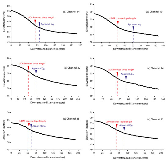
Figure 6.
Graphical representation of the longitudinal slope profile for channels 14, 19, 22, 24, 28, and 41. The position on the channels’ slope profiles of the LiDAR (Laser Imaging Detection and Ranging) convex slope length and the apparent Xrh is represented with a red and blue mark, respectively. In steady-state conditions, the value of both measurements should coincide. The difference, at the studied landscape, is due to the effect of ploughing, which buries part of the head of the channels. In some cases, as seen in channel 22, small local concavities or irregularities in the DEM (Digital Elevation Model) can lead to misinterpretations of the convex-to-concave inflection point of the channels’ profile. These anomalies should decrease as the precision and point density of the LiDAR data increases.
4. Results
Table 2 shows the obtained values for the apparent Xrh and the LiDAR convex slope length for each of the 46 measured channels. Mean values are also given for catchments A, B, and C.
Table 2.
Measured values of the apparent Xrh (ridge to head of channel distance) and LiDAR convex slope length, in meters. The deviation between those values is also shown for each channel, in meters. App. Xrh = Apparent Xrh; L.C. = LiDAR convex slope length; Dev. = Deviation between the Xrh and L.C. values.
In catchment A, 25 first-order channels were measured. The apparent Xrh ranges from a maximum value of 117.3 m to a minimum value of 48 m, with a mean value of 80.9 m. This parameter shows a considerable variation and no clear tendency, with 48% of the measured values within a range of ±12.1 m from the mean value of the catchment. The ±12.1 m range is about 15% of the average apparent Xrh value of the catchment (80.9 m). The 15% range represents an arbitrary limit value used in this study in order to help evaluate the deviation of measurements from the mean value. On the other hand, the measured values for the LiDAR convex slope length range from 129.9 to 46.6 m, with a mean value of 63.3 m. Although the deviation from the maximum and minimum values appears to be higher than that of the apparent Xrh, this parameter has a more homogeneous and consistent distribution, with 68% of the measured channels within a range of ±9.5 m (15% of the average convex length value for catchment A) from the mean value.
Catchment B consists of 11 first order-channels. The mean values for both the apparent Xrh and LiDAR convex slope length are similar to the mean values obtained in catchment A, being 82.6 and 60.8 m, respectively. However, the individual values for each parameter show less variation than those obtained for catchment A. The apparent Xrh values range from 111.2 and 58.5 m, with 63.6% of the measured values within a ±12.4 m range (15% of average apparent Xrh value) from the mean value of the catchment, while the values of the LiDAR convex slope length range from 73 to 51.2 m. In this case, 72.7% of the values are within a ±9.1 m range (15% of the average convex length) from the mean value obtained for catchment B.
Similar to the other two catchments, catchment C presents a mean apparent Xrh of 83.9 m. In this catchment, we measured 10 first-order channels and obtained individual values ranging between 101.2 and 62 m. Fifty percent of those values are within a range of ±12.6 m (15% of the average apparent Xrh) from the mean value. The channels in catchment C show a smaller variation in the LiDAR convex slope length than those in catchments A and B, with up to 90% of them within a ±9.2-m range (15% of the average convex length) from the mean value of the catchment. The average value for the catchment is 61.5 m, similar to those of catchments A and B, but the individual values are constrained within a smaller range from 69.8 to 50.1 m.
Figure 7 shows the distribution of the measured values for both parameters in catchments A, B, and C.
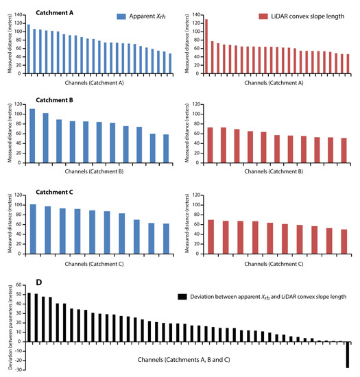
Figure 7.
(A–C) apparent Xrh and LiDAR convex slope length for each of the 46 measured first-order channels. Results are organized in catchments, and ordered from the highest to lowest value measured in each catchment; (D) deviation between the measured values of the apparent Xrh and the LiDAR convex slope length, ordered from highest to lowest value.
The apparent Xrh appears to be greater than the LiDAR convex slope length in 45 out of the 46 measured channels. The deviation between those parameters varies from one channel to another, from a maximum deviation of 51.9 m in channel 7 to a minimum of 0.8 m in channel 15 (Table 1 and Figure 7). Channel 4 is the only one with a shorter apparent Xrh than the LiDAR convex slope length. In Figure 7, this appears reflected as a negative value. Overall, the difference between the two parameters is fairly consistent for the three catchments, with mean values of 19.5, 21.8, and 22.4 m corresponding to catchments A, B, and C, respectively.
5. Discussion
The relationship between the two measurements can be seen in Figure 8. The central dashed line represents agreement between the two measurement methods, where Xrh equals the LiDAR convex slope length. The values plotted above this line represent channels where Xrh is smaller than the LiDAR convex slope length, while the values plotted under the line depict channels with higher values of Xrh than the LiDAR convex slope length.
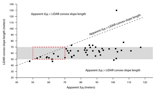
Figure 8.
Relationship between the apparent Xrh and the LiDAR convex slope length. The agreement between the two measurement methods appears represented as a dotted line. Eighty-three percent of the channels appear plotted in the grey area, representative of LiDAR convex slope length values between 50 and 70 m. Channels with apparent Xrh values within a similar range than their LiDAR convex slope length values (50 to 70 m) would be expected to appear plotted inside the red polygon.
As seen in Figure 6, 45 out of the 46 channels measured appear plotted below the line of agreement between the two measurement methods. Looking at the LiDAR convex slope length of those channels, we can see that for the most part it takes values between 50 to 70 m (82.6% of the measured channels). If those channels were near a steady-state configuration, we would expect the apparent Xrh values (measured with orthoimages) to be within a similar range, between 50 and 70 m, as both methodologies are effectively measuring the same morphometric parameter of the landform relief. However, this only occurs in a small percentage of the measured channels (19.6% of the channels). In fact, what we observe is that the apparent Xrh has a greater distribution in the upper end of the spectrum, between 70 and 120 m (78.2% of the channels) (Figure 8). These discrepancies in the results could point to changes or disturbances in the channels’ longitudinal profile that required field examination to be confirmed. Upon visual inspection of those channels in the field, it was possible to observe small channel incisions or gullies on the headwaters section of the channels’ profile, located upstream from the channel’s head (Figure 9). These incisions or gullies occur in the length between the red and blue markers in Figure 6.
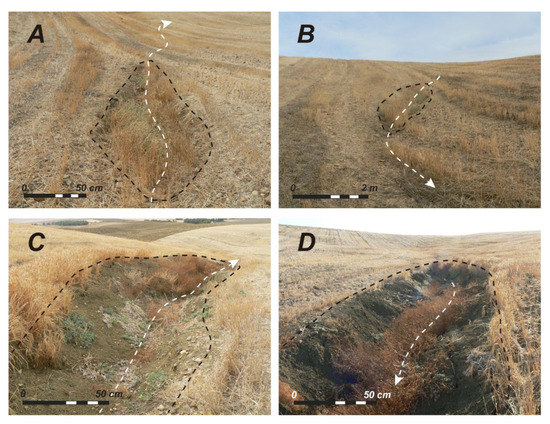
Figure 9.
Small channel incisions (inside black dashed polygons) of roughly 1 m width and 0.5 m depth, developed at the headwaters section of some channels. (A,B) Downstream and upstream views, respectively, of the channel incision developed in channel 6. (C,D) Downstream and upstream views, respectively, of the channel incision developed in channel 13. This incision develops as the channel is trying to re-establish its longitudinal profile that was obliterated by agricultural tillage. The direction of flow in each picture is represented with the white-dashed arrows.
The analysis in Figure 8 and the field observations shown in Figure 9 indicate that agricultural disturbances have modified these channels’ headwater reaches. Intensive ploughing smoothed the landscape. The mid to low sections of drainage networks developed in those areas are usually not obliterated by ploughing because the stream section depth prevents the farming equipment going through it. However, in the headwater reaches of catchments where the stream depth is not too great, agricultural machinery can traverse and obliterate these shallower channel reaches. This shortens the channels’ apparent total length (increases the apparent Xrh), while maintaining the overall convex-concave shape of the slope profile. This disturbance is not a one-time occurrence that immediately preceded the field visit. Instead, repeated annual ploughing consistently obliterates any channel reach or sign of headward erosion that the plough can traverse, maintaining the apparent head of the channels at the greater distance from the water divide throughout the years, and conceivably extending it over time as more sediment moves downslope towards the channel. This prevents the channels from fully developing their longitudinal profiles (Figure 10). The difference in the measured parameters beyond the line of agreement between the two measurement methods reflects this disturbance. Active erosion processes in the upper sections of the catchments will appear as a consequence of the channels trying to regain their lost channel length. These field observations reinforce the idea that the apparent Xrh measured from the orthoimages are, in fact, not the real steady-state values, but Xrh values that have been disrupted by agriculture.
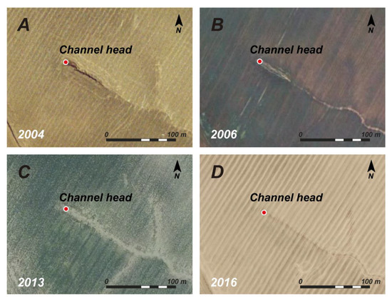
Figure 10.
(A–D) orthoimages of channel 17 (catchment A) captured in 2004, 2006, 2013, and 2016, respectively. The channel’s head appears at almost the same location in all four orthoimages. The channel’s cross section has become filled and the topography flattened in this section throughout the years due to the effect of repeated annual ploughing.
This is an important aspect to consider when identifying reference areas anywhere that land has been ploughed during agriculture or reshaped for other uses. In those areas, if ploughing or grading removed some of the channels’ headwater lengths, an erroneously longer apparent Xrh will usually be measured when identifying the channel head location from orthoimages. The comparison and analysis of results obtained with different remote sensing tools can help identify if this deviation is present and assess the validity of a catchment for obtaining input parameters for a geomorphic reclamation project. In catchments A, B, and C, the mean apparent Xrh are 80.9, 82.6, and 83.9 m, respectively. However, these apparent Xrh values are the product of agricultural activity. Under undisturbed, steady-state conditions, the real Xrh values should more closely resemble those obtained for the LiDAR convex slope length (mean values of 63.3, 60.8, and 61.5 m for catchments A, B, and C, respectively). The difference between the two values (19.5, 21.8, and 22.4 m) represents the length of the channel section obliterated by ploughing. In terms of the percentage of missing channel, this means an average 15.1%, 13.7%, and 32.4% of the total length of first-order channels for catchments A, B, and C, respectively (Table 3).
Table 3.
Length of the 46 measured first-order channels, in meters. The section of the channels obliterated by agricultural activity is represented as missing channel length, in meters and percentages. Mean M.C.L. (%) = average value of the total missing channel length for each catchment (in percentage).
If the input parameters collected from those catchments were to be used as reference areas in a geomorphic reclamation project, we would expect the final reclamation design to experience active erosion processes in order to adjust to its approximate steady-state conditions by eroding headwards to add the missing channel length. This would compromise the overall success of the design and potentially increase the post-reclamation site maintenance costs. The significance of this missing channel length will depend on the characteristics of the reclamation project. In lower gradient projects, the eroded valleys may be very shallow and not present a significant problem, whereas in projects developed on steeper terrain, the same valley length could produce a much greater and problematic amount of erosional adjustment. It is also worth noting that, although agricultural activity has a significant impact in the length of first-order channels, it has a lesser influence on the overall drainage density value of the catchment. As an example, in catchments A, B, and C, the missing channel length only represents a reduction of 5.2%, 5.7%, and 6.9% in the drainage density values, respectively (Table 4).
Table 4.
Effect of agricultural activity on the drainage density values of catchments A, B, and C. Expected steady-state condition values have been obtained by adding the total missing channel length of each catchment to the agricultural disturbed values (the values measured in this study). Total channel length is expressed in km, and the drainage density in km/km2.
The effect in the drainage density may be reduced as the catchment area increases because bigger catchments may have a larger number of high order channels unaffected by agricultural activity. In those cases, the headwaters channel section obliterated by ploughing will be comparatively smaller in relation to the total channel length of the catchment, therefore reducing the impact on drainage density values.
Considerations on Remote Sensing Tools
Remote sensing and LiDAR technology have been proven to be invaluable tools in geomorphology since their introduction. The availability of highly accurate and cost-effective elevation data that those methodologies provide has transformed, and will continue to transform, how geomorphologists study landscape form and evolution [35]. Detailed topographic information is essential in a great variety of research fields, from the morphometric analysis of river basins to erosion assessment studies.
However, even though LiDAR data and high-resolution aerial orthoimages can be extremely useful for mapping and modelling, they still require field verification and ground truthing. In this study, both methodologies have been proved to be able to adequately identify and measure the morphometric parameter of the headwater section of the catchments. These methodological procedures have the advantage of allowing a greater number of sites to be evaluated in a given period, saving both time and economic resources. Nevertheless, field visits to the reference area are still recommended to confirm the validity of estimated measurements using remote sensing data. A potential GeoFluv user that only measured the apparent Xrh in catchments A, B, and C without visiting the reference area would not be aware of ongoing adjustments in the channel network, as active signs of erosion are not easily seen in orthoimages.
This study suggests that these tools can support two tasks: they can be used to measure preliminary Xrh values and those values can be compared to provide an indication of the degree of development to a steady-state condition. As seen in Figure 8, the comparison of remote sensing methodologies can help to recognize discrepancies in the results and identify which channels (and catchments) are more valid for the collection of input parameters. This can be used as a scanning tool when several reference areas are being considered in a reclamation project, narrowing down the most suitable areas and preventing unnecessary field visits.
If a thorough remote sensing analysis indicates that a proposed reference area is likely stable, then it may be appropriate to make a conceptual fluvial geomorphic design using the input values obtained this way. However, this study supports the practice of only using field-verified input values to make an actual constructible design to assure the desired fluvial-geomorphic functionality in the reclamation design.
6. Conclusions
The analysis of the ridge to head of channel distance (Xrh) in three catchments using high-precision LiDAR data and orthoimages showed inconsistency in the values obtained using the two remote sensing methods. In natural, undisturbed conditions, the apparent Xrh value measured with orthoimages should be equivalent to the LiDAR convex slope length. In the three catchments, however, the apparent Xrh has been found to be 19.5 to 22.4 m greater (on average) than the LiDAR convex slope length of the channel erosional profile. The discrepancy between the two measurement methods was resolved by ground-truthing that indicated that agricultural activity had modified the ridge to head of channel distance (Xrh).
Although agricultural activity did not affect the general morphology of the channels in these catchments, it had a strong influence on the headwater section of their longitudinal profiles, obliterating the first meters of the channels where the stream section depth is not too profound. The deviation found between the values obtained using the two remote sensing methodologies corresponds to this disturbance in the headwater section of the first-order channels. The comparison of the results obtained with LiDAR data and orthoimages allowed for the quantification of the effect of ploughing and tillage, which has been found to reduce first-order channel’s length by 15.1% to 32.4%. Those findings provide useful information for geomorphic reclamation projects, as deviations from expected parameter values can indicate that a proposed reference area has been disturbed, as in this case, or has not attained a stable configuration for a suitable reference area and could compromise the success of the reclamation design.
The reference areas to be used in a geomorphic reclamation project should have natural, steady-state landforms developed with similar earth materials, climate, and vegetation as the disturbed reclamation area. Remote sensing technologies can help users identify these areas and obtain preliminary measurements for use as design inputs while reducing the time and expense associated with making field visits to each prospective area. Designers may be able to measure and evaluate a greater number of possible reference areas by using these remote sensing tools. That ability can help to avoid the use of input values collected from less-than-optimal reference areas, such as those developed in agricultural or otherwise disturbed landscapes.
In conclusion, LiDAR data and orthoimages proved to be useful methodologies to estimate the preliminary input values to be used in geomorphic reclamation projects. However, limitations related to the accuracy and precision of data need to be taken into account when using a single methodology alone. Local irregularities in the DEMs derived from LiDAR data can lead to the misinterpretation of the landform relief, and small features of the landscape can be difficult to identify with orthoimages. The combined use of both methodologies, supported by ground truthing, can reduce false results and also may reveal something unseen in a single method.
Author Contributions
R.S.-D., N.B., and J.F.M.-D. contributed to the conceptualization of the study; R.S.-D. contributed to the acquisition and treatment of data; R.S.-D., N.B., and J.F.M.-D. contributed to the analysis of data; R.S.-D., N.B., and J.F.M.-D. wrote the original draft manuscript; and N.B. and J.F.M.-D. provided ongoing reviews to paper drafts. All the authors have read and agreed to the published version of the manuscript.
Funding
This research was supported by the Madrid Autonomous Region Government project REMEDINAL TE-CM S2018/EMT-4338. The co-author R.S.-D. was supported by the Tatiana Pérez de Guzmán el Bueno Foundation predoctoral scholarship.
Acknowledgments
The authors want to thank Javier Cañal, Adrián González, and Fernando Pérez-Langa for their help and assistance during field work in Seville, and Ignacio Zapico for the acquisition and treatment of the LiDAR point cloud data.
Conflicts of Interest
The authors declare no conflict of interest. The funders had no role in the design of the study; in the collection, analysis, or interpretation of data; in the writing of the manuscript; or in the decision to publish the results.
References
- Howard, E.J.; Loch, R.J.; Vacher, C.A. Evolution of landform design concepts. Trans. Inst. Min. Metall. Min. Technol. 2011, 120, 112–117. [Google Scholar] [CrossRef]
- Minister of Public Works and Government Services of Canada. The Minerals and Metals Policy of the Government of Canada. In Partnerships for Sustainable Development, Catalogue No. M37-37/1996E; Minister of Public Works and Government Services: Ottawa, ON, Canada, 1996. [Google Scholar]
- BOE. Real Decreto 975/2009, de 12 de Junio, Sobre Gestión de los Residuos de las Industrias Extractivas y de Protección y Rehabilitación del Espacio Afectado por Actividades Mineras; BOE núm. 143 de 13 junio de 2009 (BOE-A-2009-984); Ministerio de la Presidencia: Madrid, Spain, 2009; pp. 49948–49993.
- Ministerio de Minería. Ley 20551, Regula el Cierre de Faenas e Instalaciones Mineras; Biblioteca del Congreso Nacional de Chile: Valparaíso, Chile, 2011.
- Feng, Y.; Wang, J.; Bai, Z.; Reading, L. Effect of surface coal mining and land reclamation on soil properties: A review. Earth-Sci. Rev. 2019, 191, 12–25. [Google Scholar] [CrossRef]
- Ramani, R.V. Surface mining technology: Progress and prospects. Procedia Eng. 2012, 46, 9–21. [Google Scholar] [CrossRef]
- Flatley, A.; Rutherfurd, I.D.; Hardie, R. River Channel Relocation: Problems and Prospects. Water 2018, 10, 1360. [Google Scholar] [CrossRef]
- Martín-Duque, J.F.; Sanz, M.A.; Bodoque, J.M.; Lucía, A.; Martín-Moreno, C. Restoring earth surface processes through landform design. A 13-year monitoring of a geomorphic reclamation model for quarries on slopes. Earth Surf. Process. Landf. 2010, 35, 531–548. [Google Scholar] [CrossRef]
- Martín-Duque, J.F.; Zapico, I.; Oyarzun, R.; López García, J.A.; Cubas, P. A descriptive and quantitative approach regarding erosion and development of landforms on abandoned mine tailings: New insights and environmental implications from SE Spain. Geomorphology 2015, 239, 1–15. [Google Scholar] [CrossRef]
- Toy, T.J.; Chuse, W.R. Topographic reconstruction: A geomorphic approach. Ecol. Eng. 2005, 24, 29–35. [Google Scholar] [CrossRef]
- SMCRA. Surface Mining Control and Reclamation Act. In Public Law, 95–87, Statutes at Large, 91 Stat. 445. Federal Law; Department of Interior: Washington, DC, USA, 1977. [Google Scholar]
- Stiller, D.M.; Zimpfer, G.L.; Bishop, M. Application of geomorphic principles to surface mine reclamation in the semiarid West. J. Soil Water Conserv. 1980, 274–277. [Google Scholar]
- Bugosh, N. Fluvial Geomorphic Principles Applied to Mined Land Reclamation. In Proceedings of the January OSM Alternatives to Gradient Terraces Workshop; Office of Surface Mining: Farmington, NM, USA, 2000. [Google Scholar]
- Bugosh, N. Innovative Reclamation Techniques at San Juan Coal Company (or why we are doing our reclamation differently). In July Rocky Mountain Coal Mining Institute National Meeting, Copper Mountain, Colorado, 3–7 November, 2003; Rocky Mountain Coal Mining Institute: Lakewood, CO, USA, 2003. [Google Scholar]
- Bugosh, N.; Eckels, R. Restoring erosional features in the desert. Coal Age 2006, 111, 30–32. [Google Scholar]
- Carlson Software. The Carlson Software Website. Available online: http://www.carlsonsw.com/ (accessed on 24 June 2020).
- Fernández-Caliani, J.C.; Barba-Brioso, C.; González, I.; Galán, E. Heavy metal pollution in soils around the abandoned mine sites of the Iberian Pyrite Belt (southwest Spain). Water Air Soil Pollut. 2009, 200, 211–226. [Google Scholar] [CrossRef]
- Yesares, L.; Sáez, R.; Nieto, J.M.; Ruiz de Almodóvar, G.; Gómez, C.; Escobar, J.M. The Las Cruces deposit, Iberian Pyrite Belt, Spain. Ore Geol. Rev. 2015, 66, 25–46. [Google Scholar] [CrossRef]
- Olías, M.; Nieto, J.M.; Pérez-López, R.; Cánovas, C.R.; Macías, F.; Sarmiento, A.M.; Galván, L. Controls on acid mine water composition from the Iberian Pyrite Belt (SW Spain). Catena 2016, 137, 12–23. [Google Scholar] [CrossRef]
- Instituto Geológico y Minero de España, GEODE–Zona Z2600 (Cuenca del Guadalquivir y Cuencas Béticas Postorogénicas, Subbético, Cuenca de Gibraltar). Available online: http://info.igme.es/cartografiadigital/geologica/geodezona.aspx?intranet=false&Id=Z2600 (accessed on 24 June 2020).
- Bugosh, N.; Martín-Duque, J.F.; Eckels, R. The GeoFluv method for mining reclamation: Why and how it is applicable to closure plans in Chile. In Proceedings of the First International Congress on Planning for Closure of Mining Operations; Wiertz, J., Priscu, D., Eds.; Gecamin: Santiago de Chile, Chile, 2016. [Google Scholar]
- Martín-Duque, J.F.; Bugosh, N. Examples of geomorphic reclamation on mined lands of Spain. From pioneering cases to the use of the GeoFluvTM method. In Proceedings of the 2014 OSM National Technical Forum, Advances in Geomorphic Reclamation at Coal Mines, Albuquerque, NM, USA, 20–22 May 2014; Office of Surface Mining, Reclamation and Reinforcement (OSM), Department of Interior: Washington, DC, USA, 2014. [Google Scholar]
- Zapico, I.; Martín-Duque, J.F.; Bugosh, N.; Laronne, J.B.; Ortega, A.; Molina, A.; Martín-Moreno, C.; Nicolau, J.M.; Sánchez Castillo, L. Geomorphic reclamation for reestablishment of landform stability at a watershed scale in mined sites: The Alto Tajo Natural Park, Spain. Ecol. Eng. 2018, 111, 100–116. [Google Scholar] [CrossRef]
- Waygood, C. Adaptative landform design for closure. In Mine Closure 2014; Weiersbye, I., Ed.; University of Witwatersrand: Johanesburg, South Africa, 2014. [Google Scholar]
- Kelder, I.; Waygood, C. Integrating the use of natural analogues and erosion modelling. In Landform Design for Closure, Proceeding of the Mine Closure 2016, Australian Centre for Geomechanics, Perth, Australia, 15–17 March; Fourie, A., Tibbett, M., Eds.; Australian Centre for Geomechanics: Perth, Australia, 2016. [Google Scholar]
- Hancock, G.R.; Martín-Duque, J.F.; Willgoose, G.R. Geomorphic design and modelling at catchment scale for best mine rehabilitation—The Drayton mine example (New South Wales, Australia). Environ. Model. Softw. 2019, 114, 140–151. [Google Scholar] [CrossRef]
- Bugosh, N.; Epp, E.G. Evaluating Sediment Production from Native and Fluvial Geomorphic-Reclamation Watersheds at La Plata Mine. Catena 2019, 174, 383–398. [Google Scholar] [CrossRef]
- Robson, M.; Spotts, R.; Wade, R.; Erickson, W. A case history: Limestone quarry reclamation using fluvial geomorphic design techniques. In Revitalizing the Environment: Proven Solutions and Innovative Approaches, Proceedings of the 2009 National Meeting of the American Society of Mining and Reclamation, Billings, MT, USA, 30 May–5 June 2009; Barnhisel, R.I., Ed.; ASMR: Lexington, IN, USA, 2009. [Google Scholar]
- Hause, D. The Squiggly Ditch—The Third Time Around. In Proceedings of the Mid-Continent Region Natural Stream Design Workshop, Mount Vernon, VA, USA, 17–19 May 2011; Office of Surface Mining Reclamation and Enforcement: Washington, DC, USA, 2011. [Google Scholar]
- Hutson, H.J.; Thomas, R.W. Advancements in geomorphic mine reclamation design approach, Wyoming abandoned mine land, Lionkol Coal Mining District, Sweetwater County, Wyoming. J. Am. Soc. Min. Reclam. 2014, 6, 51–83. [Google Scholar] [CrossRef]
- Horton, R.E. Erosional development of streams and their drainage basins; hydrophysical approach to quantitative morphology. Bull. Geol. Soc. Am. 1945, 56, 275–370. [Google Scholar] [CrossRef]
- Dunne, T.; Leopold, L.B. Water in Environmental Planning; WH Freeman and Co.: New York, NY, USA, 1978. [Google Scholar]
- Centro Nacional de Información Geográfica (CNIG). Gobierno de España. Available online: http://centrodedescargas.cnig.es/CentroDescargas/index.jsp (accessed on 24 June 2020).
- Plan Nacional de Ortofotografía Aérea. Available online: https://pnoa.ign.es/ (accessed on 24 June 2020).
- Roering, J.J.; Mackey, B.H.; Marshal, J.A.; Sweeney, K.E.; Deligne, N.I.; Booth, A.M.; Handwerger, A.L.; Cerovski-Dariiau, C. ‘You are HERE’: Connecting the dots with airborne lidar for geomorphic fieldwork. Geomorphology 2013, 200, 172–183. [Google Scholar] [CrossRef]
© 2020 by the authors. Licensee MDPI, Basel, Switzerland. This article is an open access article distributed under the terms and conditions of the Creative Commons Attribution (CC BY) license (http://creativecommons.org/licenses/by/4.0/).