Analysis of the Relative Importance of Model Parameters in Watersheds with Different Hydrological Regimes

Abstract

Depending on the purpose of the study, aggregated hydrological models are preferred over distributed models because they provide acceptable results in terms of precision and are easy to run, especially in data scarcity scenarios. To obtain acceptable results in terms of hydrological process representativeness, it is necessary to understand and assess the models. In this study, the relative importance of the parameters of the Hydrologiska Byråns Vattenbalansavdelning (HBV) model is analyzed using sensitivity analysis to detect if the simulated processes represent the predominant hydrological processes at watershed scale. As a case study, four watersheds with different hydrological regimes (glacial and pluvial) and therefore different dominant processes are analyzed. The results show that in the case of the rivers with a glacial regime, the model performance depends highly on the snow module parameters, while in the case of the rivers with a pluvial regime, the model is sensitive to the soil and evapotranspiration modules. The results are directly related to the hydrological regime, which indicates that the HBV model, complemented by sensitivity analysis, is capable of both detecting and representing hydrological processes at watershed scale.

1. Introduction

There are various hydrological models that differ in complexity and utility [1]. Hydrological models represent the processes of a watershed in a simplified manner and can be characterized as aggregated or distributed models. Distributed models consider the spatial variability of hydrometeorological, topographical, geological, soil-type and land-use variables, among others. However, their application is limited by their complexity and calculation time and the amount of information needed. Meanwhile, aggregated models represent hydrological processes via space-averaged information, considering the watershed as a unit; that is, the parameters that represent phenomena or processes do not vary spatially in the study area. These models are simpler than distributed models and require a smaller quantity of computer resources and data than distributed models.

In many cases, aggregated models are preferred over distributed models as they provide acceptable results in terms of precision [2] with lower requirements of information [3]. This study analyzes the simplified, ten-parameter version of the Hydrologiska Byråns Vattenbalansavdelning (HBV) model [4]. The HBV model was originally developed for application in Scandinavia and since its introduction it has been used in various hydrological regimes and in more than 80 countries [5] including Switzerland [6], the United States [7], New Zealand [8], Turkey, Zimbabwe, Tanzania and Bolivia [9].

An acceptable hydrological model in terms of an objective function does not necessarily ensure the hydrological representation of the processes that occur in a watershed [10]. To ensure acceptable results in terms of representativeness of time series and hydrological processes, it is necessary to understand and assess the models using tools such as sensitivity analysis [11]. Sensitivity analysis is recognized as an essential tool for the development and assessment of environmental models [12] as it allows the study of model response behavior, helps internal processes simulated by the model to be understood and allows the impact of input data variation on model outputs to be characterized [13,14]. The three main purposes of sensitivity analysis are: classification of factors in terms of their relative sensitivity (ranking), determination of the factors that influence the uncertainty of the results (screening) and determination of value ranges that produce significant results (mapping) [15]. Studies that facilitate the selection of the most suitable analysis method are presented by Devak and Dhanya [16] and Sarrazin et al. [14]. The former authors present a critical review of sensitivity analysis and sampling methods in hydrological modeling, while Sarrazin et al. [14] focus on the selection of a suitable sample size through convergence analysis. In this study, regional sensitivity analysis (RSA) and the Monte Carlo sampling method are used. According to Wagener and Kollat [17] and Sarrazin et al. [14], RSA allows factor mapping and ranking; therefore, it can detect the parameters that most influence model performance. In addition, the Monte Carlo sampling method is considered easy to implement and suitable for hydrological modeling [16].

In conceptual models, the parameters are estimated via calibration as they cannot be measured directly [18]. In some cases, to decrease the calculation time and/or increase the precision of the model results, the values of the least-influential parameters are eliminated or set via automatic calibration algorithms. However, these mathematical methods can focus on the estimation of parameters that generate a good fit in terms of one or more objective functions without regard for the representativeness of the hydrological processes of the system [19,20]. Meanwhile, Abebe et al. [7], Zelelew and Alfredsen [21], Pianosi and Wagener [22] and Yaghoubi et al. [23] have shown that process identification can be performed using sensitivity analysis; however, an objective approach to identifying and ranking processes for characterization and the understanding of basins has not yet been developed.

The objective of this study is to analyze the relative importance of the parameters of the simplified version of the HBV hydrological model developed by Aghakouchak and Habib [4] through a regional sensitivity analysis (RSA) [24] in order to detect, rank and validate the parameters that represent the predominant hydrological processes at watershed scale. For the analysis, as a case study, four watersheds with different hydrological regimes are analyzed: two watersheds with a pluvial regime (Iñaque and Cruces rivers, Chile) and two watersheds with a glacial regime (Grey and Paine rivers, Chile).

2. Study Area

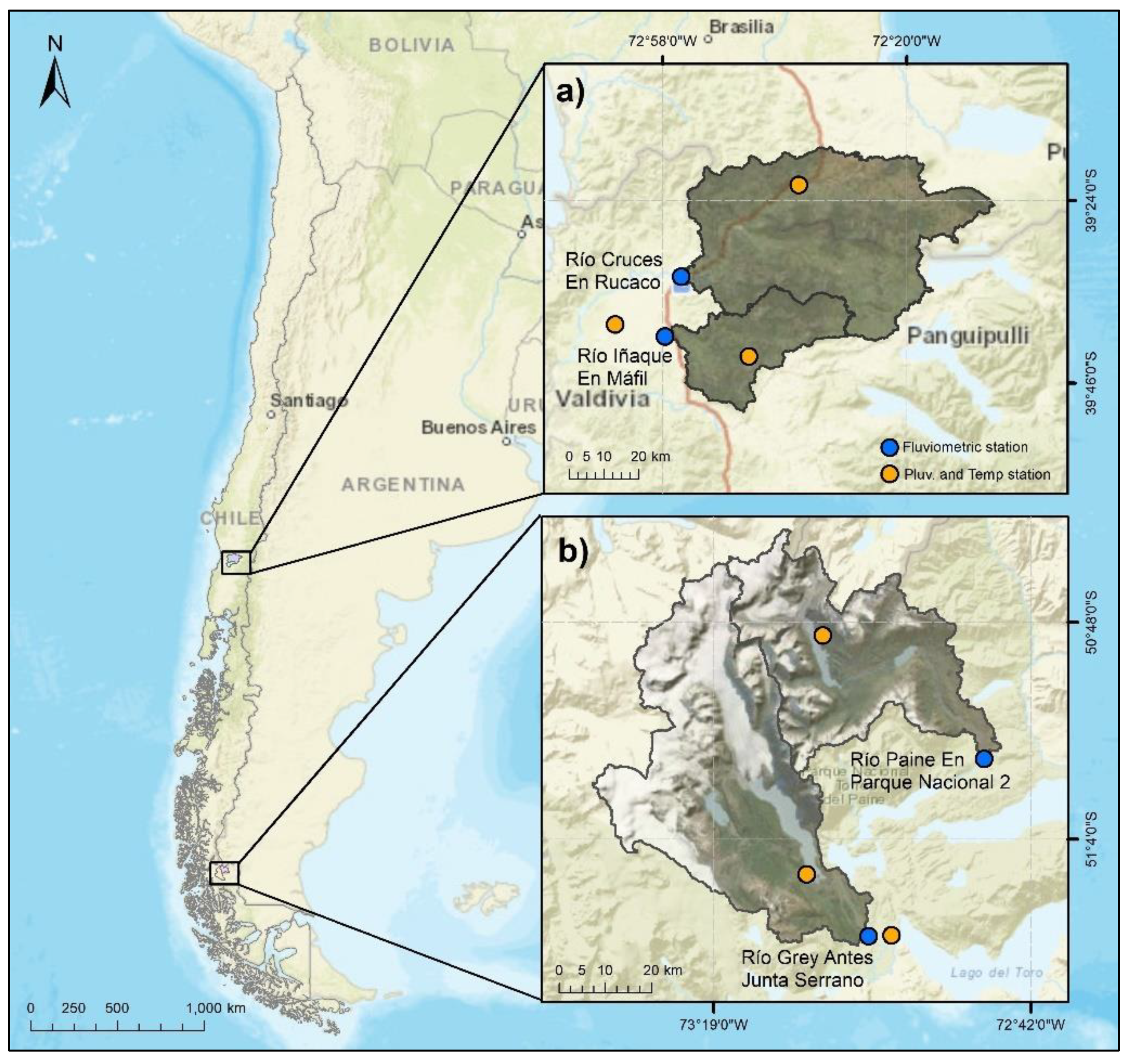
To detect the influence of different predominant hydrological processes, four watersheds with different hydrological regimes—the Iñaque, Cruces, Grey and Paine river watersheds, all located in Chile—were chosen as case studies. Each presented a simple, climate-regulated hydrological regime with variability associated with precipitation and snow and glacier melt. To validate the main process findings, two watersheds with pluvial regime and two watersheds with glacial regime were chosen.

2.1. Iñaque and Cruces Rivers

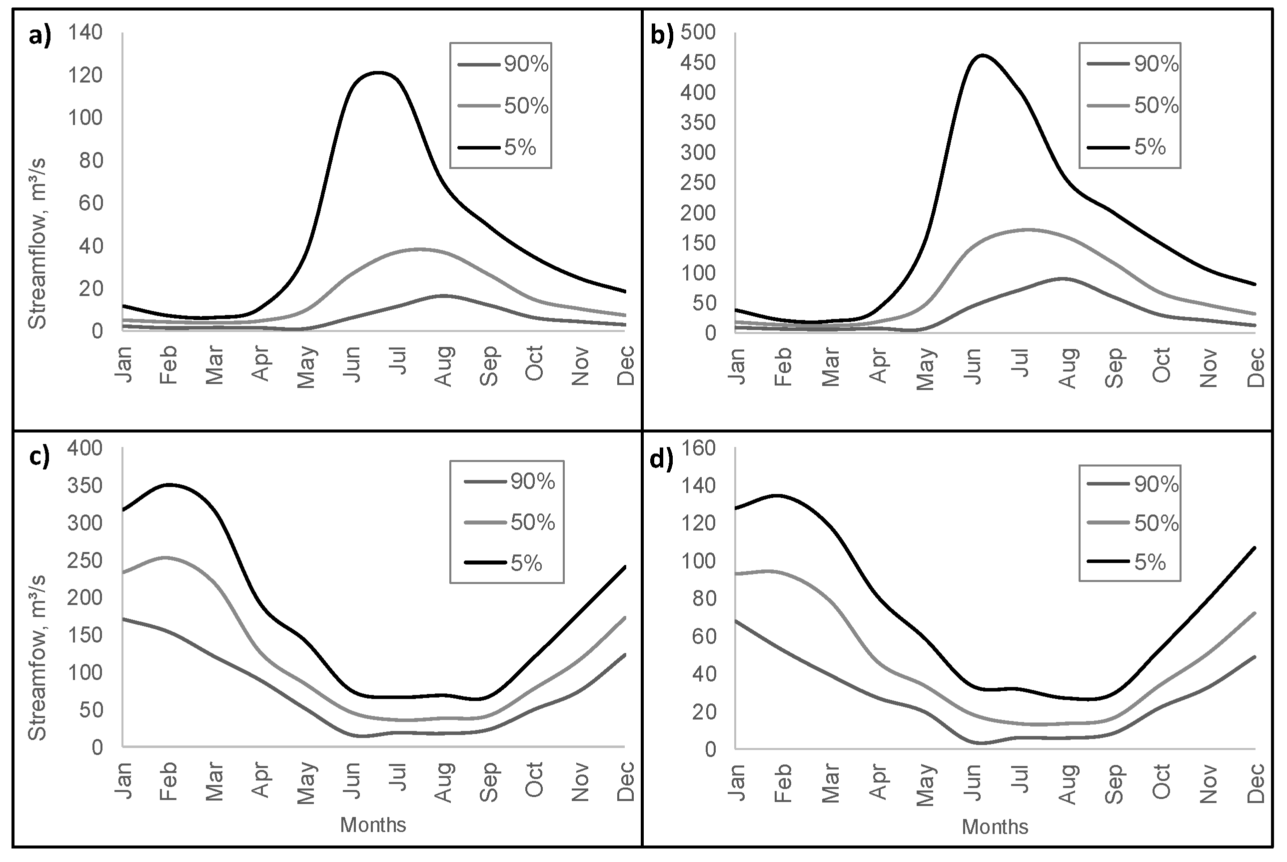
The Iñaque and Cruces river watersheds (Figure 1a) are located in the south of Chile and are monitored at the Río Iñaque En Mafil (536 km²) and Río Cruces En Rucaco streamflow station (1804 km²), respectively. Both watersheds present a rainy temperate climate with mean monthly temperatures between 6 °C and 17 °C and annual precipitation up to 1800 mm. The watersheds present a pluvial regime (Figure 2a,b), with maximum streamflows in winter (June to September). The predominant geology of the watersheds is metamorphic rock of the Paleozoic–Triassic era and sedimentary rocks of the Pleistocene–Holocene era [25].

2.2. Grey and Paine Rivers

The Grey and Paine river watersheds (Figure 1b), monitored at the Río Grey Antes Junta Serrano (918 km²) and Río Paine En Parque Nacional 2 station (583 km²), respectively, are located in the austral zone of Chile and are characterized by a tundra climate. The mean monthly temperature varies between −4 °C and 5 °C and annual precipitation can reach 1200 mm. The watersheds present runoff mainly associated with snow and glacier melt (Grey, Dickson, Cubo and Frías glaciers), exhibiting a glacial regime (Figure 2c,d). Low-permeability geological formations composed of sedimentary-volcanic sequences of the Tertiary Period stand out [26].

2.3. Data

Mean daily precipitation, mean daily temperature and monthly evapotranspiration time series representative of each watershed were required to implement the hydrological model. In this study, data from an eleven-year period (2006–2016 for Iñaque and Cruces and 2001–2011 for Grey and Paine watersheds), obtained from the online records published by the General Water Directorate (DGA, for its initials in Spanish) and Weather Service of Chile (DMC, for its initials in Spanish), were used. Based on mean monthly temperature records, monthly potential evapotranspiration (PET) was estimated using the Thornthwaite method [27].

The Thornthwaite method estimates monthly values of PET as a function of mean monthly temperature and an annual thermal index (I). According to the basin location (i.e., latitude) and number of days per month, a correction to account for the number of daylight hours and days per month is performed.

To determine the mean precipitation and temperature in the watershed, the inverse weighted distance (IWD) method was used. In addition, to compare the simulated streamflows with observations and thus apply the sensitivity analysis to identify predominant hydrological processes, streamflow records from stations controlled by the DGA from the 2006–2016 period were used.

3. HBV Hydrological Model

The HBV model [28] is a lumped snow–rainwater balance model that can be used as a lumped or semi-distributed model. In this study, the simplified version of the model presented by Aghakouchak and Habib [4] was used. This version simulated daily discharges based on daily precipitation, temperature and potential evapotranspiration time series [29].

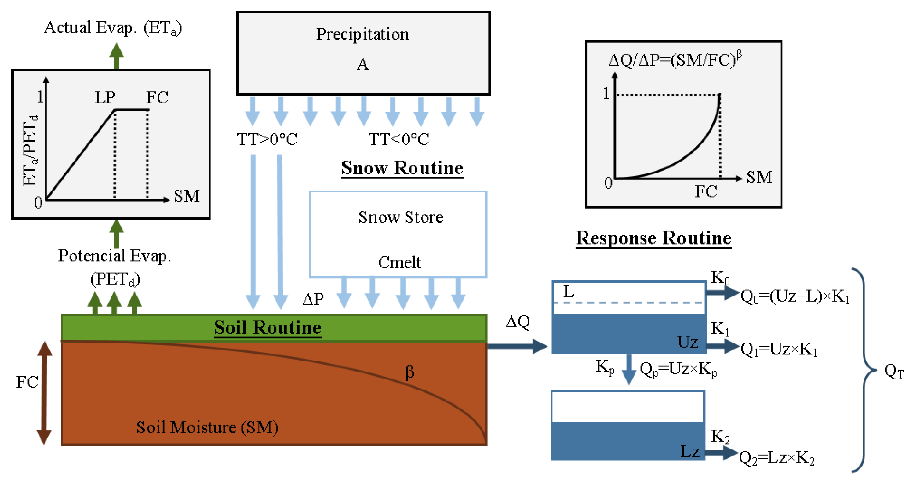
The model consisted of three main modules (see conceptual diagram in Figure 3): a snow module, an effective precipitation and soil moisture module and a response module [29]. The first module controlled snow accumulation and melting. Precipitation accumulates as snow when the temperature is below a threshold value (TT); otherwise, the model considered precipitation rain and began the snowmelt subroutine. The contribution of snowmelt to runoff was estimated through the simple degree-day method [28] depending on the difference between the actual and the threshold temperatures.

The second module determined the contribution of precipitation to infiltration and surface runoff. First, it calculated daily potential evapotranspiration (PET_d) by reducing the monthly value based on a correction factor (C), the mean daily temperature and the long-term temperature and the potential evapotranspiration averages [29]. The permanent wilting point (PWP) is a fraction (LP) of field capacity (FC); when moisture surpassed the PWP value, actual evapotranspiration (ET_a) was equal to the daily potential evapotranspiration. In addition, when soil moisture (SM) was below the PWP, a linear reduction was applied to evapotranspiration (see upper left corner of Figure 3). Subsequently, the model calculated runoff (∆Q), which depended on precipitation (∆P), soil moisture (SM), field capacity (FC) and an empirical coefficient (β), which determined the relative contribution of rain or snowmelt to runoff (see upper right corner of Figure 3).

Finally, the response model estimated the flow based on two reservoirs, one above the other. The upper reservoir represented the flow near the surface, while the lower simulated baseflow (groundwater contribution) and both were connected through a percolation rate (K_p). There were three outlets, two in the upper reservoir (Q₀ and Q₁) and one in the lower (Q₂). When the water level in the upper deposit surpassed a threshold value (L), runoff was generated quickly in its upper part (Q₀). The responses of the other two outputs were relatively slower (Q₁ and Q₂) and recession coefficients K₀, K₁ and K₂ were used to ensure that Q₀ had the quickest response and that the response of Q₂ was slower than that of Q₁. For a more detailed description of the model, consultation of Bergström [29] and Aghakouchak and Habib [4] is recommended.

In the Andes of southern Chile, a precipitation enhancement of up to three times the precipitation recorded in the lower areas may occur. Therefore, the model also included a precipitation adjustment parameter (A). This parameter allowed the model to achieve a long-term water balance [30] and thereby correct the underestimation of precipitation as a result of the lack of records in the highest parts of each watershed.

Table 1. Model parameters and ranges used for the analysis.

Parameter	Description	Range
Mass balance
A	Precipitation modification parameter	0.8–2.5
Snow module
TT (°C)	Threshold temperature that indicates the initiation of snowmelt (normally 0 °C)	0
Cmelt $\left(\mathrm{mm}°{\mathrm{C}}^{-1}{\mathrm{day}}^{-1}\right)$	Fraction of snow that melts above the threshold temperature (TT) from the beginning of snowmelt.	0.5–7
Moisture module
FC (mm)	Field capacity (storage in the soil layer)	0–2000
$\mathsf{\beta }$	Empirical coefficient that represents the soil moisture variation in the area	0–7
LP	Fraction of field capacity to calculate the permanent wilting point (PWP = LP × FC)	0.3–1
C ($°{\mathrm{C}}^{-1}$)	Correction factor for potential evapotranspiration	0.01–0.3
Response module
L (mm)	Threshold for quick runoff response	0–100
${\mathrm{K}}_0$ (${\mathrm{day}}^{-1}$)	Quick response coefficient (upper reservoir)	0.3–0.6
${\mathrm{K}}_1$ (${\mathrm{day}}^{-1}$)	Slow response coefficient (upper reservoir)	0.1–0.2
${\mathrm{K}}_2$ (${\mathrm{day}}^{-1}$)	Lower reservoir response coefficient	0.01–0.1
${\mathrm{K}}_{\mathrm{p}}$ (${\mathrm{day}}^{-1}$)	Maximum flow coefficient for percolation	0.01–0.1

presents a brief description of the parameters and initial ranges used based on the studies of Aghakouchak and Habib [4] and Kollat et al. [31].

4. Regional Sensitivity Analysis

Unlike local sensitivity analysis (LSA), which explores the variability of the model response by varying the factors around a reference value, global sensitivity analysis (GSA) attempts to assess the entire feasible space of input factors. Therefore, the choice of sample size is a critical step in sampling-based GSA (for example, RSA). If the sample is small, the analysis may not provide robust results. Meanwhile, if it is very large, it could increase the computing cost without improving the precision of the results [14].

Many of the approaches used in GSA are related to the regional sensitivity analysis method developed by Spear and Hornberger [24]. This method begins with a Monte Carlo sampling of N points in the feasible parameter space, generally extracted from a uniform distribution. The parameter sets, generated randomly, can be grouped into “behavioral” (B) and “non-behavioral” (NB) models according to a performance measure. Cumulative distribution functions (CDF) can be derived from both groups and the maximum separation between them (maximum vertical difference, MVD) can be used as an indicator of the sensitivity of the model results to the evaluated parameter; that is, it can be used as an indicator to determine whether the parameter is sensitive [17].

In this study, 15,000 (N) simulations were performed using the Monte Carlo method. The number of simulations was based on studies presented by Muñoz et al. [25] and Sarrazin et al. [14]. The models were then grouped into B and NB categories according to the Nash–Sutcliffe efficiency (NSE) [32]. The NSE was obtained via Equation (1):

$$\mathrm{NSE}=1-\frac{{{\displaystyle \sum }}_{\mathrm{t}=1}^{\mathrm{T}}{\left({\mathrm{Q}}_{\mathrm{s},\mathrm{t}}-{\mathrm{Q}}_{\mathrm{o},\mathrm{t}}\right)}^2}{{{\displaystyle \sum }}_{\mathrm{t}=1}^{\mathrm{T}}{\left({\mathrm{Q}}_{\mathrm{o},\mathrm{t}}-{\overline{\mathrm{Q}}}_{\mathrm{o}}\right)}^2}$$

(1)

where ${\mathrm{Q}}_{\mathrm{s},\mathrm{t}}, {\mathrm{Q}}_{\mathrm{o},\mathrm{t}} \mathrm{and} {\overline{\mathrm{Q}}}_{\mathrm{o}}$ are the simulated streamflow at instant t, the observed streamflow at instant t and the average of the observed streamflows, respectively. Meanwhile, T is the length of the time series. This is one of the most used performance measures in hydrology and is focused on model errors at high streamflows, underestimating model performance during low-flow conditions [33]. NSE values vary between −∞ and 1, with 1 being the optimal value. A model was considered B when the value of the objective function (NSE) was equal to or greater than 0.6, while NSE values below 0.6 were considered NB.

To validate the results, the data series were divided into two six-year periods, one for calibration and analysis (2001–2006 for Paine and Grey and 2006–2011 for the Iñaque and Cruces watersheds) and one for the validation of findings (2006–2011 for Paine and Grey and 2011–2016 for the Iñaque and Cruces watersheds). In addition, according to Seibert and Vis [34], one year of warm-up was sufficient for accommodating the initial values of hydrological models and thus eliminating their influence on the results or period of interest. Therefore, the first year of each simulation was used as a warm-up and the results in that period were discarded from the analysis of this study.

Table 2. Warm-up, calibration and validation periods used for each watershed of the study.

River Basin	Calibration Warm-Up	Calibration Period	Validation Period
Iñaque and Cruces	2006	2007–2011	2012–2016
Grey and Paine	2001	2002–2006	2007–2011

summarizes the warm-up, calibration and validation periods considered.

5. Results and Discussion

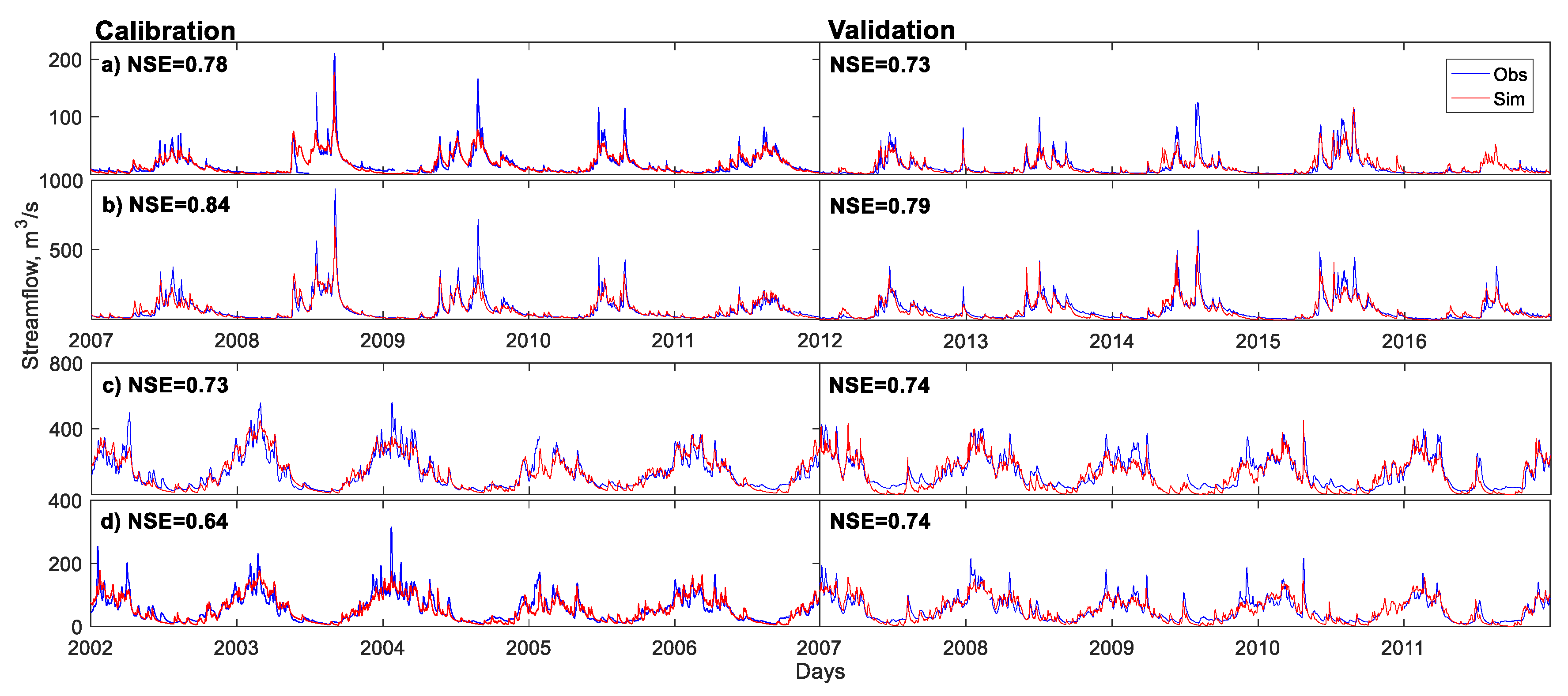
In Figure 4 the best simulation of each period as a function of the NSE value is shown. The values obtained in all watersheds indicated that the model was capable of simulating daily mean streamflows (NSE > 0.64).

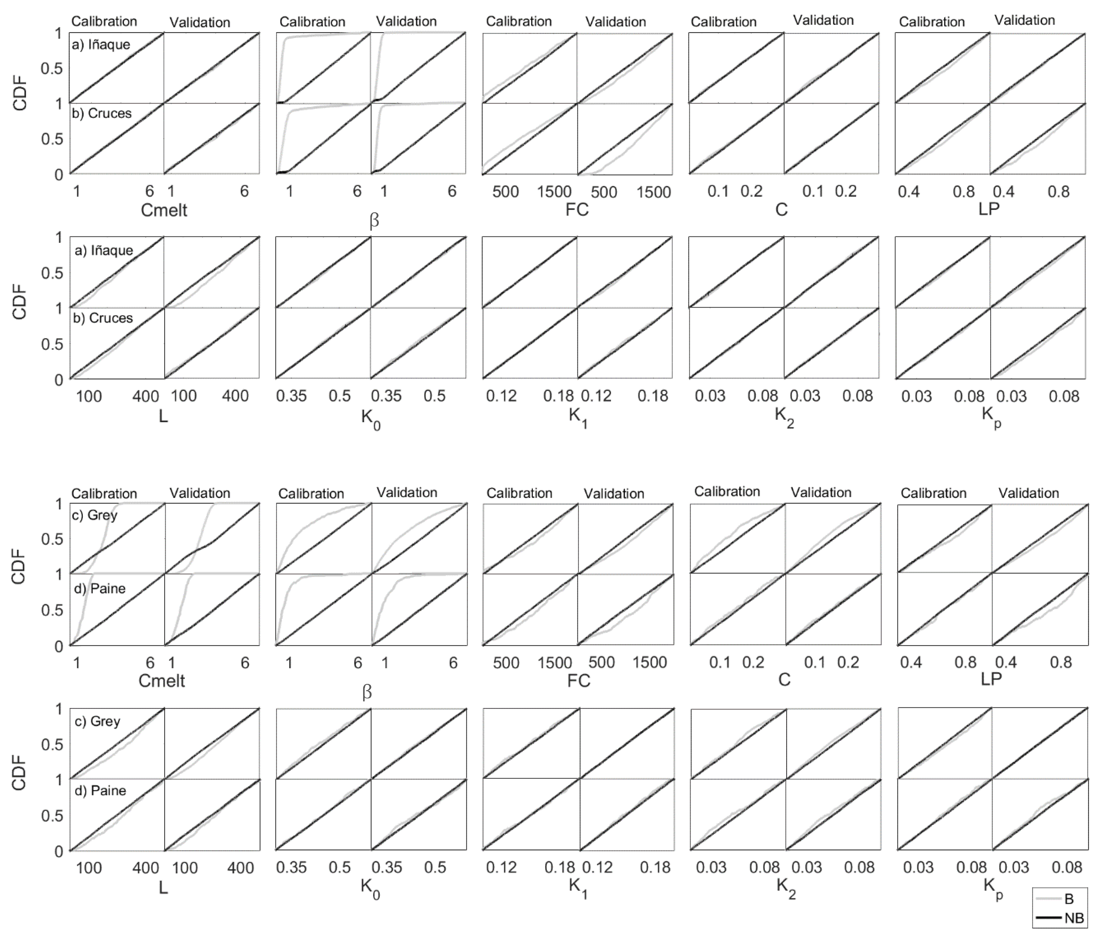
In Figure 5 the cumulative distribution functions of the regional sensitivity analysis are shown. The grey CDFs correspond to the B models, while the black CDFs correspond to the NB models.

The parameters that showed both curves (B and NB) together were not considered influential on model performance. In this case, the MVD was close to zero as the B and NB models proved insensitive to the values of the analyzed parameter. Therefore, the MVD values close to zero suggested insensitivity of the model results to the analyzed parameter. By contrast, the parameters that separated B and NB cumulative distribution functions (i.e., MVD greater than zero) were interpreted as parameters that influenced the quality of the model outputs and thus the values of the objective function. According to the CDFs, the Iñaque and Cruces river results showed that the model was sensitive to parameters $\mathsf{\beta }$, FC and L. Meanwhile, the Grey and Paine rivers results showed that the model was sensitive to parameters Cmelt, $\mathsf{\beta }$ and L.

In the Iñaque and Cruces river results, it was observed that the B models were concentrated among $\mathsf{\beta }$ values between 0.1–1. The Grey and Paine river results showed that the values of the parameter Cmelt that generated B models were in the 1–3 range $\left(\mathrm{mm}°{\mathrm{C}}^{-1}{\mathrm{d}}^{-1}\right)$ and the values of parameter $\mathsf{\beta }$ that did so were concentrated below 1.5. Parameter L values below 300 (mm) generated NB models.

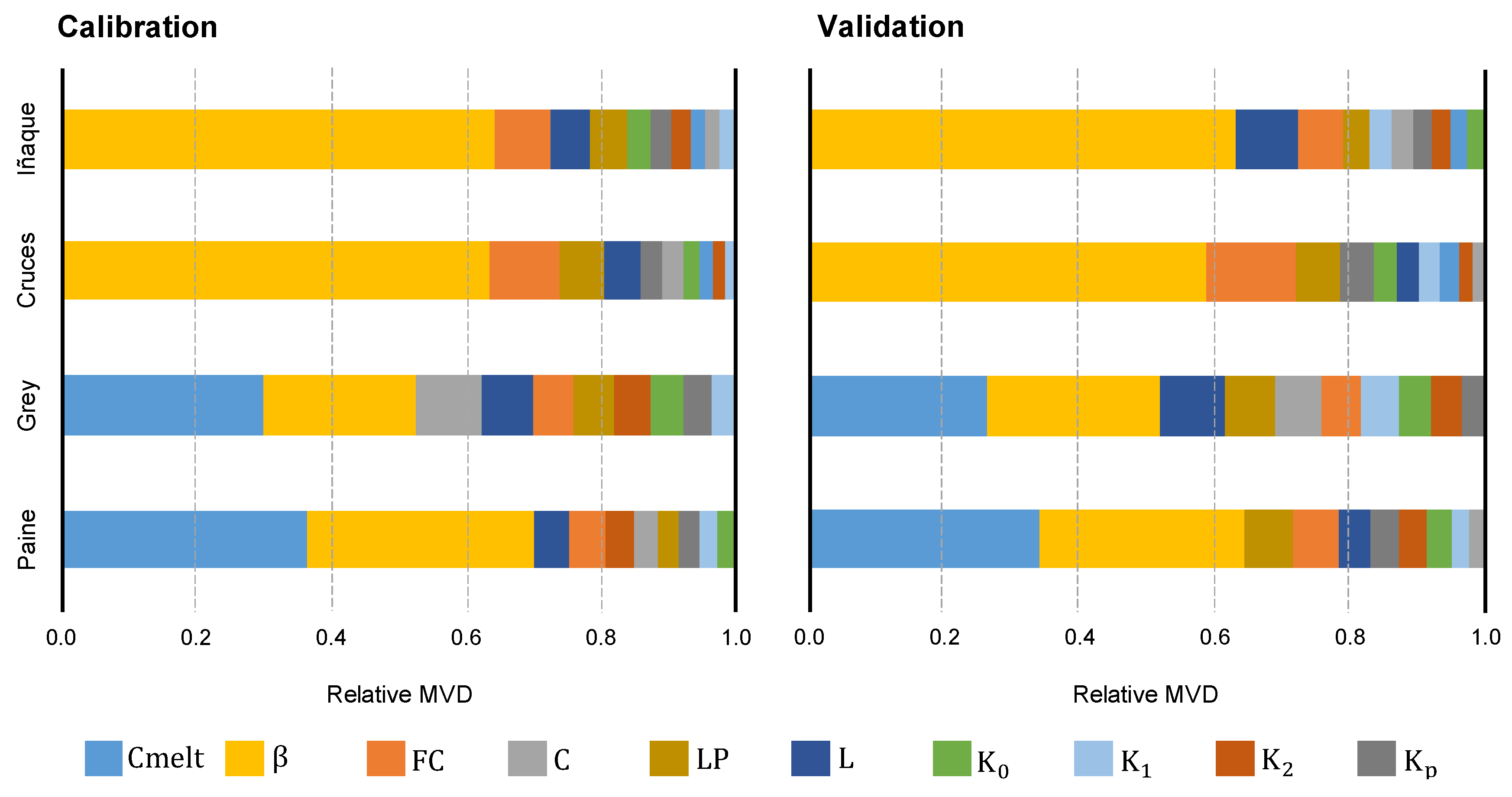
Figure 6 shows a ranking of the HBV model parameters according to the MVD sensitivity index. The relative importance of the MVD of the model parameters is shown from the most important on the left to least important on the right. The most sensitive parameters in the case of the Iñaque and Cruces River watersheds (pluvial regime) were $\mathsf{\beta }$ and FC. $\mathsf{\beta }$ represented soil moisture variation and FC was part of the soil module and represented the maximum soil moisture storage. Meanwhile, the least sensitive were Cmelt, ${\mathrm{K}}_1$ and ${\mathrm{K}}_2$ (recession coefficients). The validation stage allowed us to reach the same conclusion, with a slight change in the relative importance of L for the Iñaque River; however, L was also directly related to soil moisture storage as it defined the water threshold for a quick response. Therefore, the results also showed that the main processes for the Iñaque and Cruces basins were those related to the soil routine.

In the case of the Grey and Paine river watersheds (glacial regime), it was observed that the model was more sensitive to the parameters Cmelt and $\mathsf{\beta }$. The first was part of the snow module and the second was the soil module. Cmelt was the fraction of snow that melted and suggested that the dominant processes in the Grey and Paine basins were those related to snow accumulation and melt. $\mathsf{\beta }$, on the other hand, was related to the surface runoff process. Therefore, soil moisture and surface runoff processes were of secondary importance in glacial basins such as the Grey and Paine watersheds. The same results could be found in the calibration and validation periods in the four basins, suggesting that the utilized approach was adequate for the purposes of process ranking and identification.

The main input to the Grey and Paine rivers is melt from the Grey Glacier and Dickson, Cubo and Frías glaciers, respectively. This was represented in the sensitivity of the model to the Cmelt parameter, which controlled the snow input (in this case, glacial) to total runoff. Snow accumulation partially or completely impedes infiltration; therefore, processes related to soil moisture and runoff were of secondary importance. In the cases of the Iñaque and Cruces river watersheds, the main input is pluvial; therefore, soil moisture and evapotranspiration were the processes (present in the model) that took on the greatest importance in the model. As it had no snow input, the model was not sensitive to the parameter Cmelt.

In both cases (pluvial and glacial regimes), the model presented a high sensitivity to the $\mathsf{\beta }$, as in other studies (for example, Abebe et al. [7] and Zelelew and Alfredsen [21]) but in the case of the glacial watershed, $\mathsf{\beta }$ took slightly lower values than in the pluvial watershed. Braun and Renner [6] applied the HBV model in watersheds with different hydrological regimes and stated that the greatest differences were observed in $\mathsf{\beta }$. In addition, they concluded that it was possible to apply the model in watersheds with different characteristics but, like Bergström [35], stated that the physical interpretations of the model parameters were vague. More recently, Pianosi and Wagener [22] performed a time-varying sensitivity analysis (PAWN method) of parameter groups in the HBV model applied in a snow-affected, wet and arid watershed. The results showed that the model did detect certain characteristics of each watershed (as a function of the sensitivity of the model to the parameters); in the first (snow), it presented greater sensitivity to the snow module parameters and in the others to the response module (wet) and soil module (arid).

6. Conclusions

The HBV model was implemented in two watersheds with a pluvial regime and another two watersheds with a glacial regime and an RSA was used to analyze the relative importance of the model parameters.

In accordance with the results of the study, the regional sensitivity analysis allowed the relative importance of the HBV model parameters to be detected, generating a ranking that enabled the identification of the predominant hydrological processes in watersheds with different hydrological regimes. In the watersheds with a glacial regime (Grey and Paine rivers), the parameters with the greatest influence were those that represented the snowmelt process (Cmelt), while in the watersheds with the pluvial regime (Iñaque and Cruces rivers), soil moisture variation ($\mathsf{\beta }$) stood out. In both cases, the model parameters that presented the greatest sensitivity were directly related to the hydrological regime of each watershed and its predominant hydrological processes. The main input to the Grey and Paine river watersheds is from the Grey, Dickson, Cubo and Frías glaciers and the main input to the Iñaque and Cruces river watersheds is pluvial. In addition, the best simulation values according to the NSE confirmed that it is possible to use the simplified version of the HBV model in watersheds with different hydrological regimes.