A User-Friendly Software Package to Develop Storm Water Management Model (SWMM) Inputs and Suggest Low Impact Development Scenarios
Abstract
1. Introduction
2. Materials and Methods
2.1. Study Area Description and Stormwater Sampling
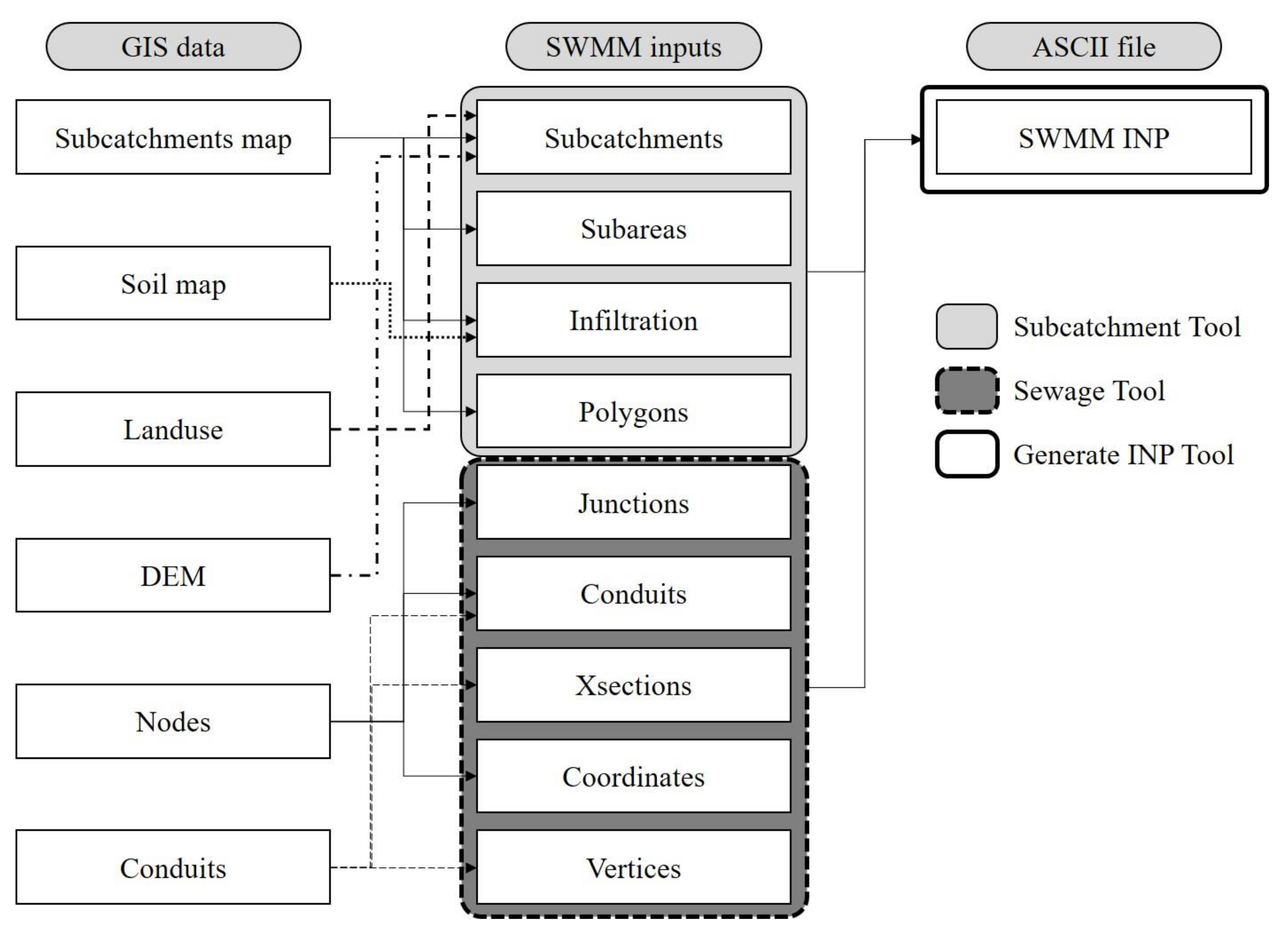
2.2. SWMM Model Description and Input Preparation Using Geographical Information System (GIS) Data
2.3. Optimizing Approach for LIDs
3. Results and Discussion
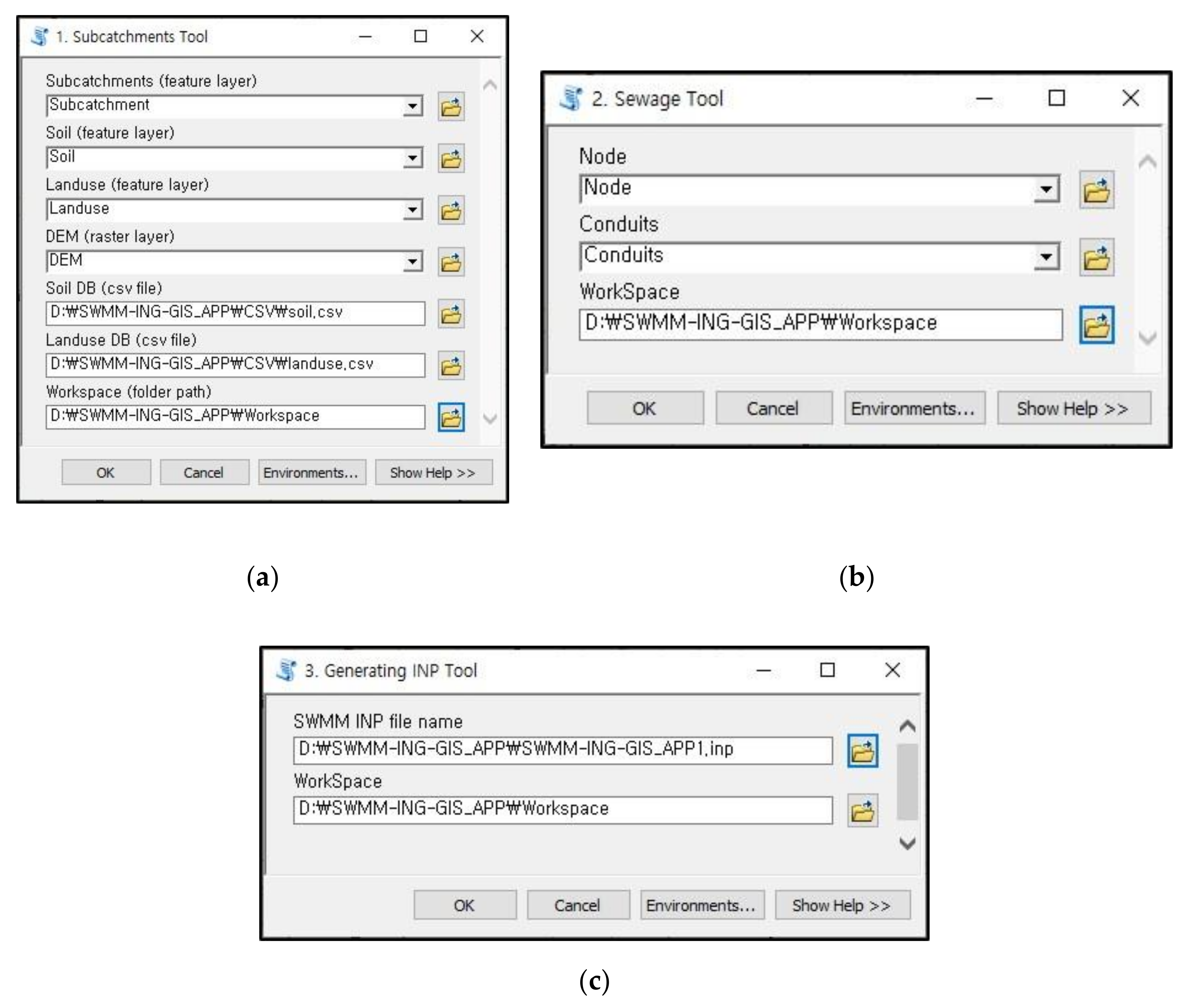
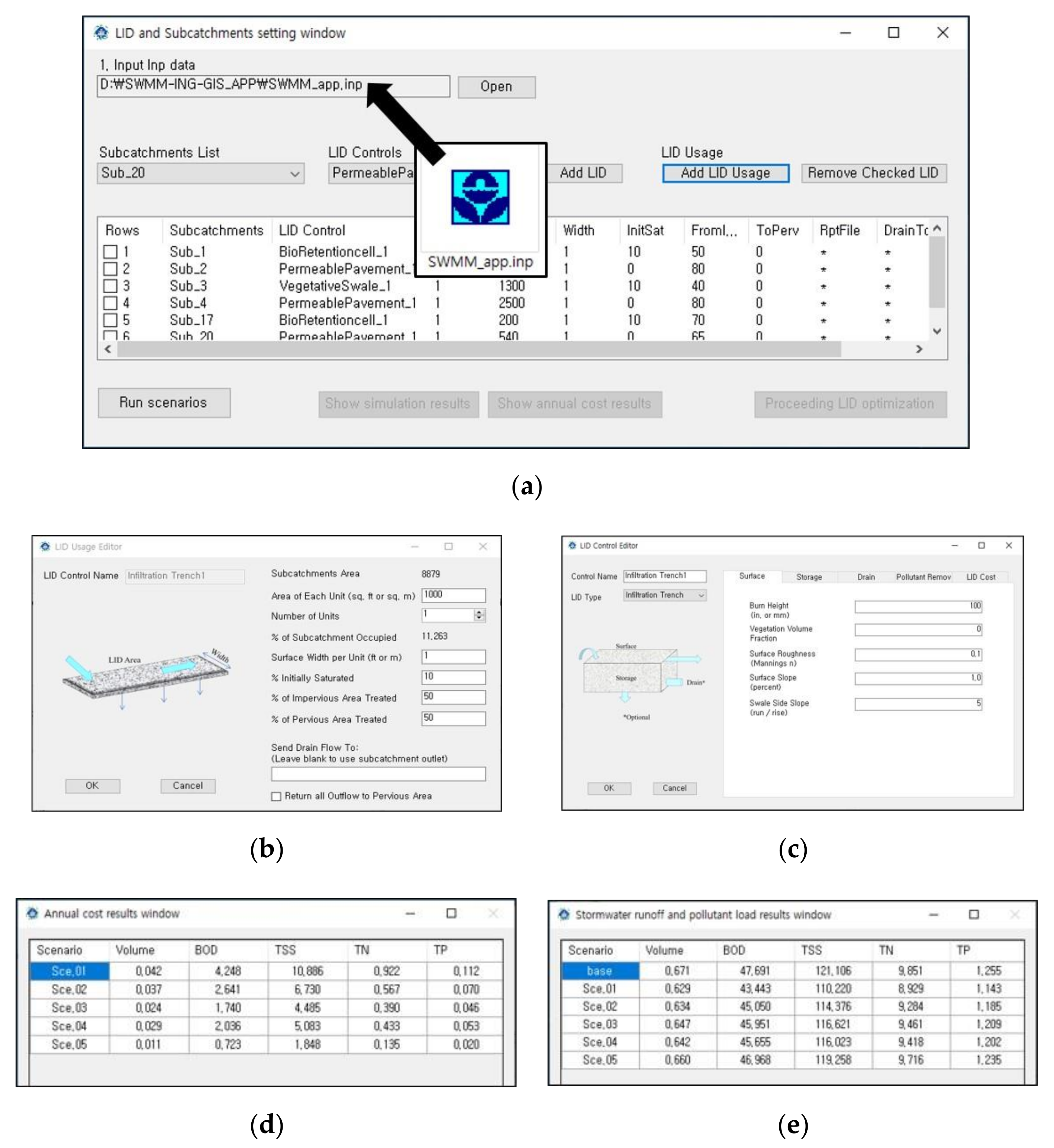
3.1. Interfaces of User-Friendly Software Package for SWMM Model
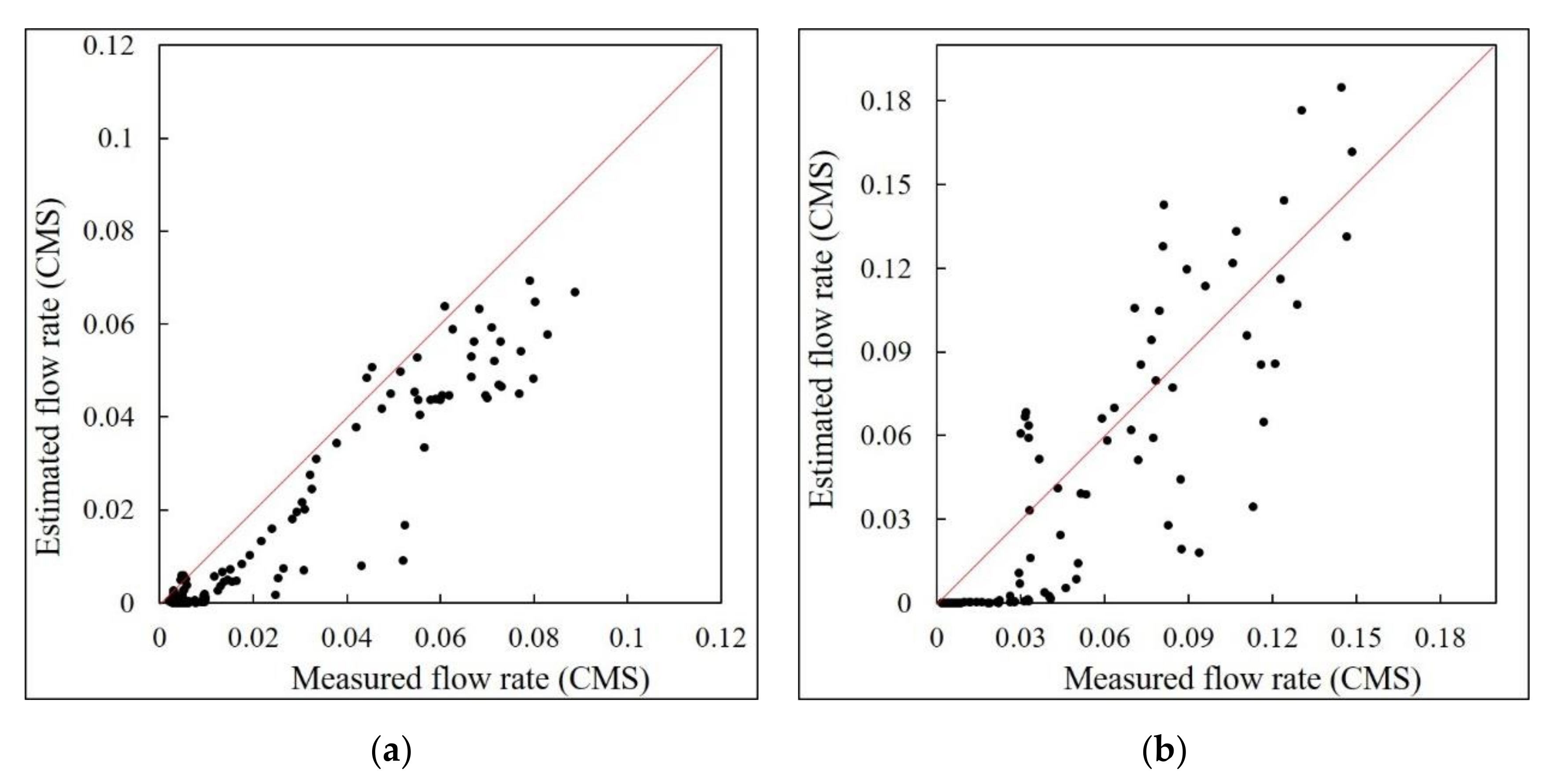
3.2. Calibration and Validation of SWMM Model
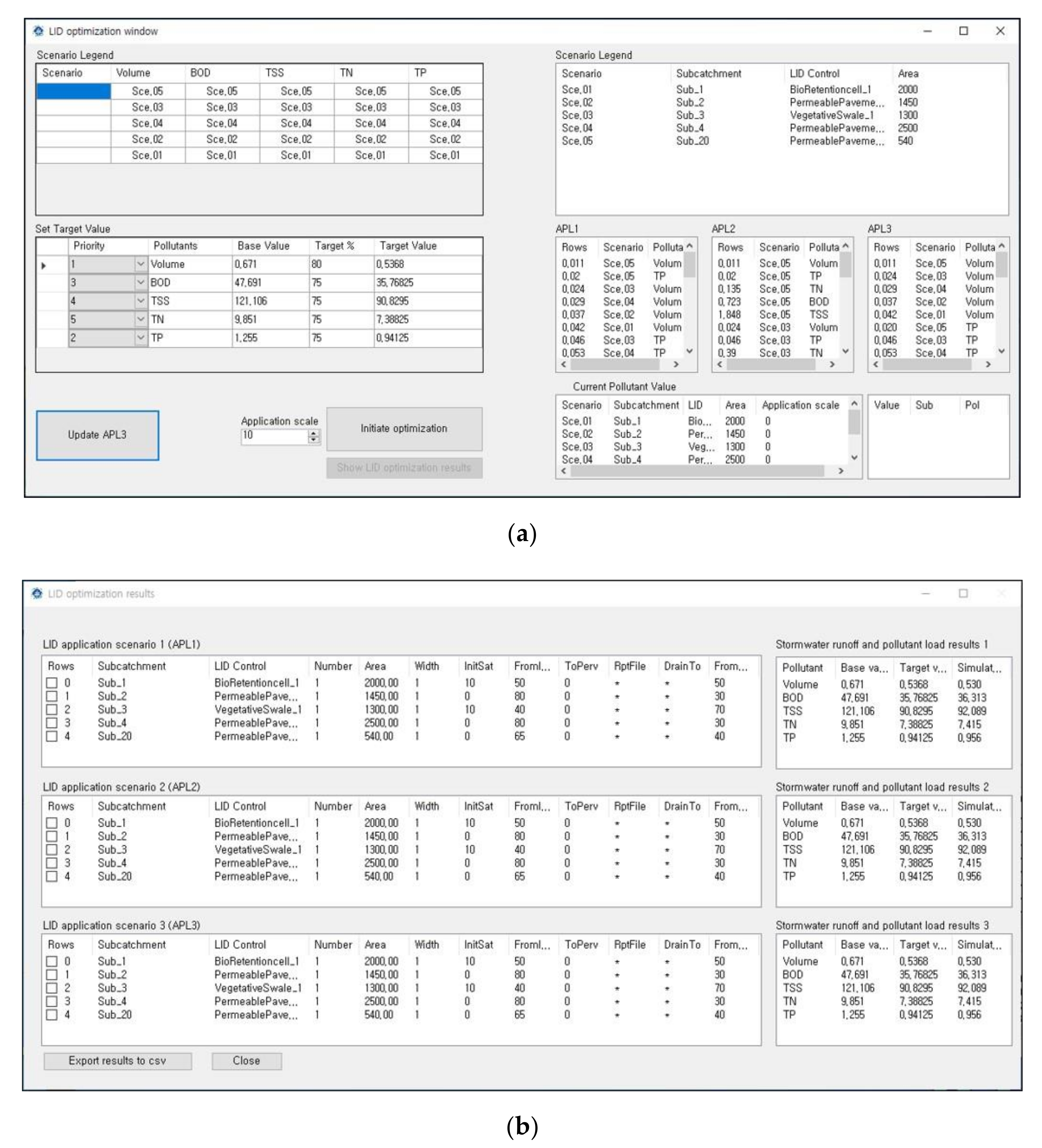
3.3. Development of Cost-Effective LID Scenarios
4. Conclusions
- It provides user convenience by applying a graphical user interface.
- The existing input data of the SWMM model can be used.
- Optimization of LID method for stormwater runoff and multiple NPS pollution is possible.
- Placement based on the size of the applied LID practice and the target area is possible.
- Annual costs, including establishment cost, maintenance cost, interest rate, and life cycle, are considered.
- Because the optimization process is not complicated, users will have a clear understanding of the approach.
Author Contributions
Funding
Acknowledgments
Conflicts of Interest
References
- Shuster, W.D.; Bonta, J.; Thurston, H.; Warnemuende, E.; Smith, D.R. Impacts of impervious surface on watershed hydrology: A review. Urban Water J. 2005, 2, 263–275. [Google Scholar] [CrossRef]
- Dietz, M.E. Low impact development practices: A review of current research and recommendations for future directions. Water Air Soil Pollut. 2007, 186, 351–363. [Google Scholar] [CrossRef]
- Ahiablame, L.M.; Engel, B.; Chaubey, I. Effectiveness of low impact development practices: Literature review and suggestions for future research. Water Air Soil Pollut. 2012, 223, 4253–4273. [Google Scholar] [CrossRef]
- Ahiablame, L.M.; Engel, B.; Chaubey, I. Effectiveness of low impact development practices in two urbanized watersheds: Retrofitting with rain barrel/cistern and porous pavement. J. Environ. Manag. 2013, 119, 151–161. [Google Scholar] [CrossRef]
- Line, D.E.; Brown, R.A.; Hunt, W.F.; ASCE, M.; Lord, W.G. Effectiveness of LID for commercial development in North Carolina. J. Environ. Eng. 2012, 138, 680–688. [Google Scholar] [CrossRef]
- Liu, Y.; Bralts, V.F.; Engel, B.A. Evaluating the effectiveness of management practices on hydrology and water quality at watershed scale with a rainfall-runoff model. Sci. Total Environ. 2015, 511, 298–308. [Google Scholar] [CrossRef]
- Kirkpatrick, S.; Gelatt, C.D.; Vecchi, M.P. Optimization by simulated annealing. Science 1983, 220, 671–680. [Google Scholar] [CrossRef]
- Baek, S.S.; Choi, D.H.; Jung, J.W.; Lee, H.J.; Lee, H.; Yoon, K.S.; Cho, K.H. Optimizing low impact development (LID) for stormwater runoff treatment in urban area, Korea: Experimental and modeling approach. Water Res. 2015, 86, 122–131. [Google Scholar] [CrossRef]
- Chen, C.F.; Sheng, M.Y.; Chang, C.L.; Kang, S.F.; Lin, J.Y. Application of the SUSTAIN model to a watershed-scale case for water quality management. Water 2014, 6, 3575–3589. [Google Scholar] [CrossRef]
- Huang, C.L.; Hsu, N.S.; Liu, H.J.; Huang, Y.H. Optimization of low impact development layout designs for megacity flood mitigation. J. Hydrol. 2018, 564, 542–558. [Google Scholar] [CrossRef]
- Kaini, P.; Artita, K.; Nicklow, J.W. Optimizing structural best management practices using SWAT and genetic algorithm to improve water quality goals. Water Resour. Manag. 2012, 26, 1827–1845. [Google Scholar] [CrossRef]
- Lee, J.G.; Selvakumar, A.; Alvi, K.; Riverson, J.; Zhen, J.Z.; Shoemaker, L.; Lai, F. A watershed-scale design optimization model for stormwater best management practices. Environ. Model. Softw. 2012, 37, 6–18. [Google Scholar] [CrossRef]
- Liu, Y.; Cibin, R.; Bralts, V.F.; Chaubey, I.; Bowling, L.C.; Engel, B.A. Optimal selection and placement of BMPs and LID practices with a rainfall-runoff model. Environ. Model. Softw. 2016, 80, 281–296. [Google Scholar] [CrossRef]
- Park, Y.S.; Engel, B.A.; Harbor, J. A web-based model to estimate the impact of best management practices. WATER 2014, 6, 455–471. [Google Scholar] [CrossRef]
- Seo, M.; Jaber, F.; Srinivasan, R.; Jeong, J. Evaluating the impact of low impact development (LID) practices on water quantity and quality under different development designs using SWAT. Water 2017, 9, 193. [Google Scholar] [CrossRef]
- Zhang, G.; Hamlett, J.M.; Reed, P.; Tang, Y. Multi-objective optimization of low impact development designs in an urbanizing watershed. Open J. Optim. 2013, 2, 95–108. [Google Scholar] [CrossRef]
- Rossman, L.A. Modeling Low Impact Development Alternatives with SWMM. J. Water Manag. Model. 2010, 6062, 167–182. [Google Scholar] [CrossRef]
- Holland, J.H. Adaptation in Natural and Artificial Systems; MIT Press: Cambridge, MA, USA, 1975. [Google Scholar]
- Vrugt, J.A.; Robinson, B.A. Improved evolutionary optimization from genetically adaptive multi-method search. Proc. Nat. Acad. Sci. USA 2007, 104, 708–711. [Google Scholar] [CrossRef]
- Tetra Tech, Inc. User’s Guide Spreadsheet Tool for the Estimation of Pollutant Load (STEPL) Version 4.1; Tetra Tech, Inc.: Fairfax, VA, USA, 2011. [Google Scholar]
- Arabi, M.; Govindaraju, R.S.; Hantush, M.M. Cost-effective allocation of watershed management practices using a genetic algorithm. Water Resour. Res. 2006, 42, W10429. [Google Scholar] [CrossRef]
- Deb, K.; Pratap, A.; Agarwal, S.; Meyarivan, T. A fast and elitist multiobjective genetic algorithm: NSGAII. IEEE Trans. Evolutionary Computation 2002, 6, 182–197. [Google Scholar] [CrossRef]
- Barco, J.; Wong, K.M.; Stenstorm, M.K. Automatic calibration of the U.S. EPA SWMM model for a large urban catchment. J. Hydro. Eng. 2008, 134, 466–474. [Google Scholar] [CrossRef]
- Choi, K.; Ball, J.E. Parameter estimation for urban runoff modelling. Urban Water 2002, 4, 31–41. [Google Scholar] [CrossRef]
- Chow, M.F.; Yusop, Z.; Toriman, M.E. Modelling runoff quantity and quality in tropical urban catchment using Storm Water Management Model. Int. J. Environ. Sci. Technol. 2012, 9, 737–748. [Google Scholar] [CrossRef]
- Borris, M.; Viklander, M.; Gustafsson, A.M.; Marsalek, J. Modelling the effects of changes in rainfall event characteristics on TSS loads in urban runoff. Hydrol. Process 2014, 28, 1787–1796. [Google Scholar] [CrossRef]
- Temprano, J.; Arango, Ó.; Cagiao, J.; Suárez, J.; Tejero, I. Stormwater quality calibration by SWMM: A case study in Northern Spain. Water SA 2006, 32, 55–63. [Google Scholar] [CrossRef]
- Zare, S.O.; Saghafian, B.; Shamsai, A. Multi-objective optimization for combined quality-quantity urban runoff control. Hydrol. Earth Syst. Sci. 2012, 16, 4531–4542. [Google Scholar] [CrossRef]
- Goncalves, M.L.R.; Zischg, J.; Rau, S.; Sitzmann, M.; Rauch, W. Modeling the effects of introducing low impact development in a tropical city: A case study from Joinville, Brazil. Sustainability 2018, 10, 728. [Google Scholar] [CrossRef]
- Vaillancourt, C.; Duchesne, S.; Pelletier, G. Hydrologic performance of permeable pavement as an adaptive measure in urban area: Case studies near Montreal, Canada. J. Hydro. Eng. 2019, 24, 05019020. [Google Scholar] [CrossRef]
- Baek, S.S.; Ligaray, M.; Pyo, J.; Park, J.P.; Kang, J.H.; Pachepsky, Y.; Chun, J.A.; Cho, K.H. A novel water quality module of the SWMNM model for assessing low impact development (LID) in urban watersheds. J. Hydrol. 2020, 586, 124886. [Google Scholar] [CrossRef]
- U.S. EPA. Storm Water Management Model User’s Manual Version 5.1; United States Environmental Protection Agency: Cincinnati, OH, USA, 2015. [Google Scholar]
- ESRI. ArcGIS for Desktop; Version 10.3; Environmental Systems Research Institute: Redlands, CA, USA, 2015; Available online: http://www.esri.com/ (accessed on 1 July 2020).
- Engel, B.; Storm, D.; White, M.; Arnold, J.; Arabi, M. A hydrologic/water quality model application protocol. J. Am. Water Resour. Assoc. 2007, 43, 1223–1236. [Google Scholar] [CrossRef]
- Moriasi, D.N.; Gitau, M.W.; Pai, N.; Daggupati, P. Hydrologic and water quality models: Performance measures and evaluation criteria. Am. Soc. Agric. Biol. Eng. 2015, 58, 1763–1785. [Google Scholar] [CrossRef]
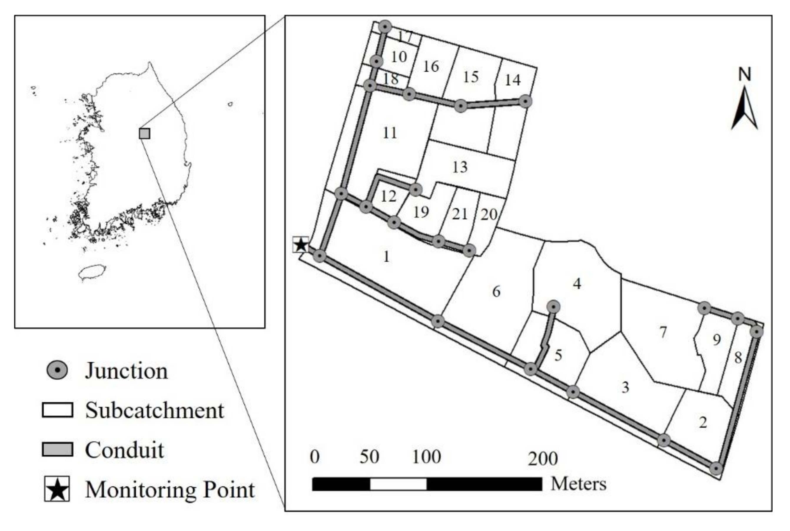
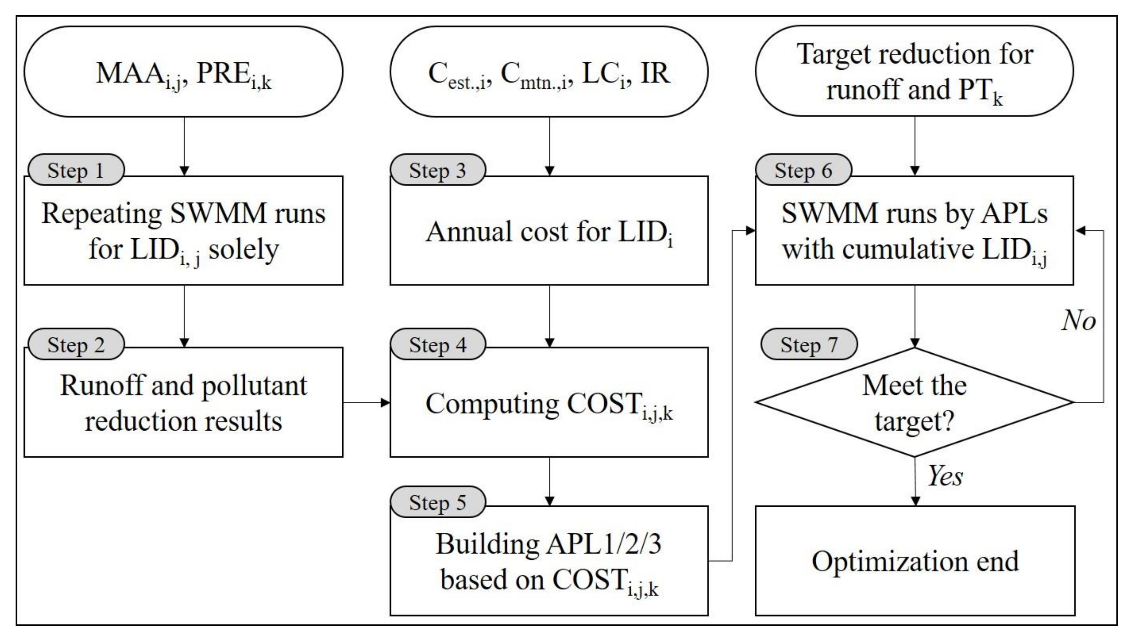
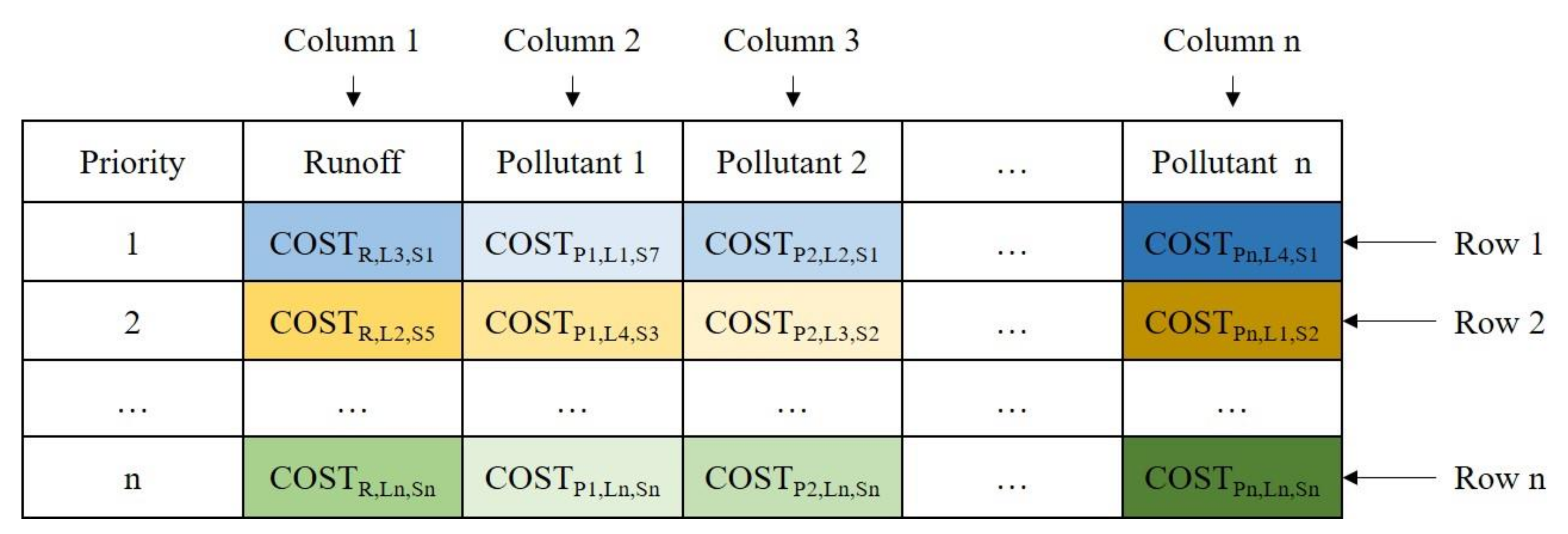
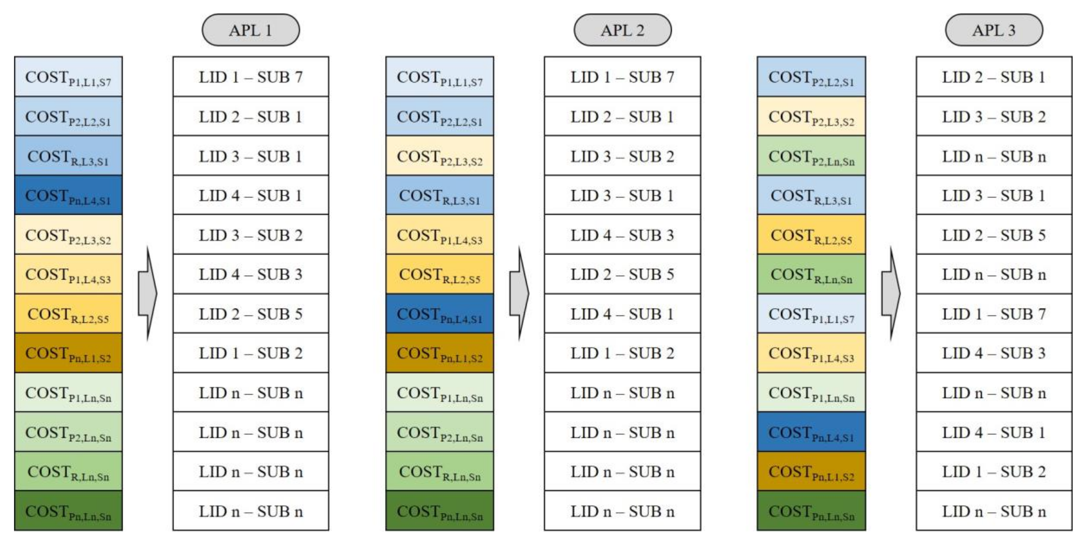
| Sub-catchment | Area (ha) | Slope (%) | Soil | ||
|---|---|---|---|---|---|
| Total | Pervious | Impervious | |||
| 1 | 0.8879 | 0.0883 | 0.7996 | 2.86 | Silt loam |
| 2 | 0.3493 | 0.0069 | 0.3424 | 4.90 | Loam |
| 3 | 0.5236 | 0.1400 | 0.3836 | 20.44 | Loam |
| 4 | 0.5385 | 0.2780 | 0.2605 | 26.88 | Loam |
| 5 | 0.3464 | 0.0568 | 0.2896 | 15.64 | Loam |
| 6 | 0.6601 | 0.0635 | 0.5966 | 4.32 | Silt loam |
| 7 | 0.5075 | 0.0651 | 0.4424 | 9.04 | Loam |
| 8 | 0.1751 | 0.0000 | 0.1751 | 6.80 | Loam |
| 9 | 0.1813 | 0.0000 | 0.1813 | 7.71 | Loam |
| 10 | 0.1241 | 0.0071 | 0.1170 | 3.09 | Silt loam |
| 11 | 0.6302 | 0.0000 | 0.6302 | 3.34 | Silt loam |
| 12 | 0.1275 | 0.0046 | 0.1229 | 3.60 | Silt loam |
| 13 | 0.2980 | 0.0526 | 0.2454 | 3.65 | Silt loam |
| 14 | 0.2443 | 0.0207 | 0.2236 | 3.51 | Loam |
| 15 | 0.3872 | 0.0911 | 0.2961 | 3.53 | Silt loam |
| 16 | 0.1776 | 0.0413 | 0.1363 | 3.20 | Silt loam |
| 17 | 0.0428 | 0.0000 | 0.0428 | 2.91 | Silt loam |
| 18 | 0.0787 | 0.0143 | 0.0644 | 3.90 | Silt loam |
| 19 | 0.1708 | 0.0389 | 0.1319 | 3.45 | Silt loam |
| 20 | 0.1074 | 0.0032 | 0.1042 | 3.43 | Silt loam |
| 21 | 0.1342 | 0.0258 | 0.1084 | 3.44 | Silt loam |
| Total | 6.6925 | 0.9982 | 5.6943 | - | - |
| SWMM Input Items | Input Details | GIS Data |
|---|---|---|
| Sub-catchments | Physical characteristics of sub-catchment (imperviousness, width, slope, etc.) | Sub-catchments map, soil map, land use, digital elevation model (DEM) |
| Subarea | Roughness, etc. | Sub-catchments map |
| Infiltration | Suction head, conductivity, initial deficit | Soil map |
| Polygons | Sub-catchment coordinates | Sub-catchments map |
| Junctions | Elevation, initial and maximum water depth, etc. | Sewer network map |
| Conduits | Inlet and outlet nodes, length, roughness, initial and maximum flow | Sewer network map |
| X-sections | Pipe type, pipe size, etc. | Sewer network map |
| Coordinates | Node coordinates | Sewer network map |
| Vertices | Conduit coordinates | Sewer network map |
| Suspended Solid | Total Phosphorus | |||||
|---|---|---|---|---|---|---|
| Measured (kg) | Estimated (kg) | Difference (%) | Measured (kg) | Estimated (kg) | Difference (%) | |
| Calibration | 112.51 | 97.47 | −13.37 | 0.55 | 0.60 | 8.88 |
| Validation | 146.95 | 167.90 | 14.26 | 1.26 | 1.10 | −12.73 |
| LID | Establishment Cost ($/m2) | Maintenance Cost ($/m2) | Life Cycle (Year) | Annual Cost ($/m2/Year) |
|---|---|---|---|---|
| Permeable pavement | 120 | 0.91 | 20 | 14.58 |
| Bioretention cell | 470 | 0.30 | 25 | 50.62 |
| Infiltration trench | 89 | 4.54 | 15 | 16.74 |
| Green roof | 287 | 3.78 | 50 | 52.18 |
| Sub-catchment Number | LID | Sub-catchment Area (m2) | Maximum Applicable Area (MAA) (m2) |
|---|---|---|---|
| 1 | Bioretention cell | 8879 | 1500 |
| 1 | Permeable pavement | 8879 | 4400 |
| 3 | Permeable pavement | 5236 | 2500 |
| 4 | Bioretention cell | 5385 | 1250 |
| 4 | Permeable pavement | 5385 | 2500 |
| 5 | Bioretention cell | 3464 | 900 |
| 6 | Green roof | 6601 | 1500 |
| 6 | Permeable pavement | 6601 | 3000 |
| 7 | Permeable pavement | 5075 | 3500 |
| 8 | Infiltration trench | 1751 | 500 |
| 11 | Green roof | 6302 | 3350 |
| 11 | Permeable pavement | 6302 | 2500 |
| 13 | Infiltration trench | 2980 | 1500 |
| 13 | Permeable pavement | 2980 | 1400 |
| 15 | Permeable pavement | 3872 | 1900 |
| Sub-catchment | LID | LID Area (m2) | Annual Cost ($/Year) |
|---|---|---|---|
| 3 | Permeable pavement | 2500 | 36,250 |
| 4 | Bioretention cell | 1250 | 63,275 |
| 4 | Permeable pavement | 2500 | 36,250 |
| 8 | Infiltration trench | 500 | 8375 |
| 11 | Green roof | 3350 | 175,306 |
| 11 | Permeable pavement | 500 | 7,250 |
| 13 | Infiltration trench | 1500 | 25,125 |
| 13 | Permeable pavement | 1400 | 20,300 |
| 15 | Permeable pavement | 1900 | 27,550 |
| Total | 15,400 | 399,681 |
© 2020 by the authors. Licensee MDPI, Basel, Switzerland. This article is an open access article distributed under the terms and conditions of the Creative Commons Attribution (CC BY) license (http://creativecommons.org/licenses/by/4.0/).
Share and Cite
Lee, H.; Woo, W.; Park, Y.S. A User-Friendly Software Package to Develop Storm Water Management Model (SWMM) Inputs and Suggest Low Impact Development Scenarios. Water 2020, 12, 2344. https://doi.org/10.3390/w12092344
Lee H, Woo W, Park YS. A User-Friendly Software Package to Develop Storm Water Management Model (SWMM) Inputs and Suggest Low Impact Development Scenarios. Water. 2020; 12(9):2344. https://doi.org/10.3390/w12092344
Chicago/Turabian StyleLee, Hanyong, Wonhee Woo, and Youn Shik Park. 2020. "A User-Friendly Software Package to Develop Storm Water Management Model (SWMM) Inputs and Suggest Low Impact Development Scenarios" Water 12, no. 9: 2344. https://doi.org/10.3390/w12092344
APA StyleLee, H., Woo, W., & Park, Y. S. (2020). A User-Friendly Software Package to Develop Storm Water Management Model (SWMM) Inputs and Suggest Low Impact Development Scenarios. Water, 12(9), 2344. https://doi.org/10.3390/w12092344


