An Experimental Investigation of the Hydraulics and Pollutant Dispersion Characteristics of a Model Beaver Dam


Abstract
1. Introduction and Literature Review
1.1. Background
1.2. Previous Work on Beaver Dams and Leaky Barriers
1.3. Pollution Transport Modelling
1.4. Summary
2. Experimental Set-up
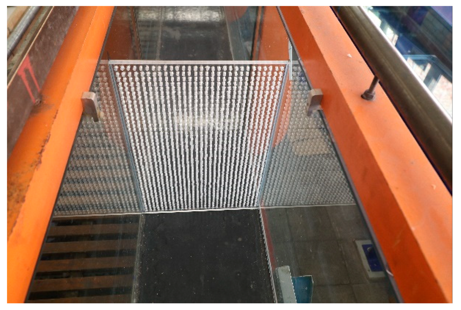
2.1. Physical Model and Discharge Measurements
2.2. Dye Tracing
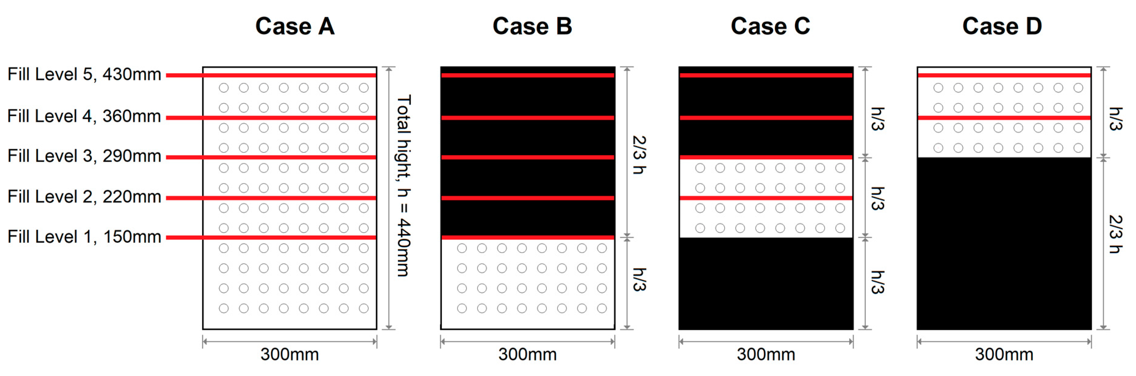
2.3. Test Program
3. Modelling Framework
3.1. Discharge Modelling
3.2. Concentration Profile Modelling
- Travel time, : The difference in centroids between the up- and down-stream distribution (t1 and t2 in Figure 5)
- The Longitudinal Dispersion Coefficient, : A mathematical quantification of how much the solute has spread between the up- and down-stream location
4. Results
4.1. Flow-Depth and Discharge Relationship
4.2. Quantification of Residence Time and Solute Concentration Distribution
5. Discussion
5.1. Model Validation
5.2. Limitations and Further Work
6. Conclusions
- A general relationship exists between flow-depth and discharge for dams with both porous and impermeable sections, provided a breakdown of the relative depths is known and accounted for.
- The residence time of dams with both porous and impermeable sections can be reasonably estimated using the Nominal Residence Time.
- A general relationship exists between flow-depth and the dimensionless Longitudinal Dispersion Coefficient for dams with both porous and impermeable sections, provided a breakdown of the relative depths is known and accounted for.
- The Advection Dispersion Equation can be used to predict a reasonable estimate of the down-stream concentration distribution of solutes for such dams.
Author Contributions
Funding
Acknowledgments
Conflicts of Interest
References
- Jackson, S.; Decker, T. Beavers in Massachusetts; University of Massachusetts–Cooperative Extension Service: Cambridge, MA, USA, 1993. [Google Scholar]
- Johnston, C.A.; Naiman, R.J. Aquatic patch creation in relation to beaver population trends. Ecology 1990, 71, 1617–1621. [Google Scholar] [CrossRef]
- Woo, M.K.; Waddington, J.M. Effects of beaver dams on subarctic wetland hydrology. Arctic 1990, 43, 223–230. [Google Scholar] [CrossRef]
- Pastor, J.; Bonde, J.; Johnston, C.; Naiman, R.J. Markovian analysis of the spatially dependent dynamics of beaver ponds. Lect. Math. Life Sci. 1993, 23, 5–27. [Google Scholar]
- Pollock, M.M.; Heim, M.; Werner, D. Hydrologic and geomorphic effects of beaver dams and their influence on fishes. Am. Fish. Soc. Symp. 2003, 37, 213–233. [Google Scholar]
- Elliott, M. Beavers return to Devon. Water Manag. 2019, 2019, 8–9. [Google Scholar]
- Labrecque-Foy, J.-P.; Morin, H.; Girona, M.M. Dynamics of Territorial Occupation by North American Beavers in Canadian Boreal Forests: A Novel Dendroecological Approach. Forests 2020, 11, 221. [Google Scholar] [CrossRef]
- Neumayer, M.; Teschemacher, S.; Schloemer, S.; Zahner, V.; Rieger, W. Hydraulic modeling of beaver dams and evaluation of their impacts on flood events. Water 2020, 12, 300. [Google Scholar] [CrossRef]
- Grygoruk, M.; Nowak, M. Spatial and Temporal Variability of Channel Retention in a Lowland Temperate Forest Stream Settled by European Beaver (Castor fiber). Forests 2014, 5, 2276–2288. [Google Scholar] [CrossRef]
- Stabler, D.F. Increasing Summer Flow in Small Streams through Management of Riparian Areas and Adjacent Vegetation—A Synthesis; USDA Forest Service General Technical Report; USDA Forest Service: Fort Collins, CO, USA, 1985; pp. 206–210.
- Briggs, M.A.; Wang, C.; Day-Lewis, F.D.; Williams, K.H.; Dong, W.; Lane, J.W. Return flows from beaver ponds enhance floodplain-to-river metals exchange in alluvial mountain catchments. Sci. Total Environ. 2019, 685, 357–369. [Google Scholar] [CrossRef]
- Westbrook, C.J.; Cooper, D.J.; Baker, B.W. Beaver dams and overbank floods influence groundwater-surface water interactions of a Rocky Mountain riparian area. Water Resour. Res. 2006, 42, W06406. [Google Scholar] [CrossRef]
- de Visscher, M.; Nyssen, J.; Pontzeele, J.; Billi, P.; Frankl, A. Spatio-temporal sedimentation patterns in beaver ponds along the Chevral river, Ardennes, Belgium. Hydrol. Process. 2013. [Google Scholar] [CrossRef]
- Butler, D.R.; Malanson, G.P. Sedimentation rates and patterns in beaver ponds in a mountain environment. Geomorphology 1995, 13, 255–269. [Google Scholar] [CrossRef]
- Hering, D.; Gerhard, M.; Kiel, E.; Ehlert, T.; Pottgiesser, T. Review: Study on near-natural conditions of central European mountain streams, with particular reference to debris and beaver dams: Results of the REG meeting 2000. Limmologica 2001, 31, 81–92. [Google Scholar] [CrossRef]
- Klotz, R.L. Reduction of high nitrate concentrations in a central New York state stream impounded by Beaver. Northeast. Nat. 2010, 17, 349–356. [Google Scholar] [CrossRef]
- Kroes, D.E.; Bason, C.W. Sediment-trapping by Beaver ponds in streams of the Mid-Atlantic Piedmont and Coastal Plain, USA. Southeast. Nat. 2015, 14, 577–595. [Google Scholar] [CrossRef]
- Kasahara, T.; Wondzell, S.M. Geomorphic controls on hyporheic exchange flow in mountain streams. Water Resour. Res. 2003, 39, 1005. [Google Scholar] [CrossRef]
- Lautz, L.K.; Siegel, D.I.; Bauer, R.L. Impact of debris dams on hyporheic interaction along a semi-arid stream. Hydrol. Process. 2006, 20, 183–196. [Google Scholar] [CrossRef]
- Wondzell, S.M. Effect of morphology and discharge on hyporheic exchange flows in two small streams in the Cascade Mountains of Oregon, USA. Hydrol. Process. 2006, 20, 267–287. [Google Scholar] [CrossRef]
- Gooseff, M.N.; Hall, R.O.J.; Tank, J.L. Relating transient storage to channel complexity in streams of varying land use in Jackson Hole, Wyoming. Water Resour. Res. 2007, 43, W01417. [Google Scholar] [CrossRef]
- Jin, L.; Siegel, D.I.; Lautz, L.K.; Otz, M.H. Transient storage and downstream solute transport in nested stream reaches affected by beaver dams. Hydrol. Process. 2009, 23, 2438–2449. [Google Scholar] [CrossRef]
- Hester, E.T.; Doyle, M.W. In-stream geomorphic structures as drivers of hyporheic exchange. Water Resour. Res. 2008, 44, W03417. [Google Scholar] [CrossRef]
- Leakey, S.; Hewett, C.J.M.; Glenis, V.; Quinn, P.F. Modelling the Impact of Leaky Barriers with a 1D Godunov-Type Scheme for the Shallow Water Equations. Water 2020, 12, 371. [Google Scholar] [CrossRef]
- Meentemeyer, R.; Butler, D. Hydrogeomorphic effects of beaver dams in Glacier National Park, Montana. Phys. Geogr. 1999, 20, 436–446. [Google Scholar] [CrossRef]
- Elliot, A.H. Settling of fine sediment in a channel with emergent vegetation. J. Hydraul. Eng. 2000, 126, 570–577. [Google Scholar] [CrossRef]
- Braskerud, B.C. The influence of vegetation on sedimentation and resuspension of soil particles in small constructed wetlands. J. Environ. Qual. 2001, 30, 1447–1457. [Google Scholar] [CrossRef] [PubMed]
- Carollo, F.G.; Ferro, V.; Termini, D. Flow velocity measurements in vegetated channels. J. Hydraul. Eng. 2002, 128, 664–673. [Google Scholar] [CrossRef]
- Pollock, M.; Beechie, T.; Jordan, C. Geomorphic changes upstream of beaver dams in Bridge Creek, an incised stream channel in the interior Columbia River basin, eastern Oregon. Earth Surf. Process. 2007, 32, 1174–1185. [Google Scholar] [CrossRef]
- McCullough, M.; Eisenhauer, D.; Dosskey, M.; Admiraal, D. Modeling beaver dam effects on ecohydraulics and sedimentation in an agricultural watershed. In Publications from USDA-ARS/UNL Faculty—Paper 145; American Society of Agricultural and Biological Engineers: St. Joseph Charter Township, MI, USA, 2007; Volume 11. [Google Scholar] [CrossRef]
- Green, K.; Westbrook, C. Changes in riparian area structure, channel hydraulics, and sediment yield following loss of beaver dams. J. Ecosyst. Manag. 2009, 10, 68–79. [Google Scholar]
- Wolman, M.G.; Miller, J.P. Magnitude and frequency of forces in geomorphic processes. J. Geol. 1960, 68, 54–74. [Google Scholar] [CrossRef]
- Daniels, M.D.; Rhoads, B.L. Effect of large woody debris configuration on three-dimensional flow structure in two low-energy meander bends at varying stages. Water Resour. Res. 2004, 40, W11302. [Google Scholar] [CrossRef]
- Rasche, D.; Reinhardt-Imjela, C.; Schulte, A.; Wenzel, R. Hydrodynamic simulation of the effects of stable in-channel large wood on the flood hydrographs of a low mountain range creek, Ore Mountains, Germany. Hydrol. Earth Syst. Sci. 2019, 23, 4349–4365. [Google Scholar] [CrossRef]
- Smith, D.L.; Allen, J.B.; Eslinger, O.; Valeciano, M.; Nestler, J.; Goodwin, R.A. Hydraulic Modeling of Large Roughness Elements with Computational Fluid Dynamics for Improved Realism in Stream Restoration Planning. In Stream restoration in dynamic fluvial systems: Scientific approaches, anaylses, and tools. Geophys. Monogr. Ser. 2011, 194, 115–122. [Google Scholar]
- Addy, S.; Wilkinson, M.E. Representing natural and artificial in-channel large wood in numerical hydraulic and hydrological models. Wires Water 2019, 6, e1389. [Google Scholar] [CrossRef]
- Milledge, D.; Odoni, N.; Allott, R.; Evans, M.; Pilkington, M.; Walker, J. Annex 6. Flood risk modelling. In Restoration of Blanket Bogs; FloodRisk Reductionand Other Ecosystem Benefits; Pilkington, M., Ed.; Moors for the Future Partnership: Edale, UK, 2015. [Google Scholar]
- Metcalfe, P.; Beven, K.; Hankin, B.; Lamb, R. A modelling framework for evaluation of the hydrological impacts of nature-based approaches to flood risk management, with application to in-channel interventions across a 29-km2 scale catchment in the United Kingdom. Hydrol. Process. 2017, 31, 1734–1748. [Google Scholar] [CrossRef]
- Cabaneros, S.; Danieli, F.; Formetta, G.; Gonzalez, R.; Grinfield, M.; Hankin, B.; Hewitt, I.; Johnstone, T.; Kamilova, A.; Kovacs, A.; et al. JBA Trust Challenge: A Risk-Based Analysis of Small Scale, Distributed, “Nature-Based” Flood Risk Management Measures Deployed on River Networks; Technical Report Maths Foresees: Leeds, UK, 2018. [Google Scholar]
- Bencala, K.E.; Mcknight, D.M.; Zellweger, G.W. Characterization of transport in an acidic and metal-rich mountain stream based on a lithium tracer injection and simulations of transient storage. Water Resour. Res. 1990, 26, 989–1000. [Google Scholar] [CrossRef]
- Bencala, K.E.; Walters, R.A. Simulation of Solute Transport in a Mountain Pool-and-Riffle Stream: A Transient Storage Model. Water Resour. Res. 1983, 19, 718–724. [Google Scholar] [CrossRef]
- Jackman, A.; Walters, R.; Kennedy, V. Transport and concentration controls for Chloride, Strontium, potassium and lead in Uvas Creek, a small cobble-bed stream in Santa Clara County, California, USA: 2, Mathematical modeling. J. Hydrol. 1984, 75, 111–141. [Google Scholar] [CrossRef]
- Czernuszenko, W.; Rowinski, P.-M.; Sukhodolov, A. Experimental and numerical validation of the dead-zone model for longitudinal dispersion in rivers. J. Hydraul. Res. 1998, 36, 269–280. [Google Scholar] [CrossRef]
- Singh, S.K. Treatment of stagnant zones in river in advection-dispersion. J. Hydraul. Eng. 2003, 129, 470–473. [Google Scholar] [CrossRef]
- Moghaddam, M.B.; Mazaheri, M.; Vali Samani, J.M. A comprehensive one-dimensional numerical model for solute transport in rivers. Hydrol. Earth Syst. Sci. 2017, 21, 99–116. [Google Scholar] [CrossRef]
- D’Angelo, D.; Webster, J.; Gregory, S.; Meyer, J. Transient storage in Appalachian and Cascade mountain streams as related to hydraulic characteristics. J.N. Am. Benthol. Soc. 1993, 223–235. [Google Scholar] [CrossRef]
- De Angelis, D.; Loreau, M.; Neergaard, D.; Mulholland, P.; Marzolf, E. Modelling nutrient-periphyton dynamics in streams: The importance of transient storage zones. Ecol. Modell. 1985, 80, 149–160. [Google Scholar] [CrossRef]
- Morrice, J.A.; Valett, H.; Dahm, C.N.; Campana, M.E. Alluvial characteristics, groundwater–surface water exchange and hydrological retention in headwater streams. Hydrol. Process. 1997, 11, 253–267. [Google Scholar] [CrossRef]
- Van Mazijk, A.; Veling, E. Tracer experiments in the Rhine Basin: Evaluation of the skewness of observed concentration distributions. J. Hydrol. 2005, 307, 60–78. [Google Scholar] [CrossRef]
- Wörman, A.; Kronnäs, V. Effect of Pond Shape and Vegetation Heterogeneity on Flow and Treatment Performance of Constructed Wetlands. J. Hydrol. 2005, 301, 123–138. [Google Scholar] [CrossRef]
- Jenkins, G.A.; Greenway, M. The hydraulic efficiency of fringing versus banded vegetation in constructed wetlands. Ecol. Eng. 2005, 25, 61–72. [Google Scholar] [CrossRef]
- Min, J.H.; Wise, W.R. Simulating short-circuiting flow in a constructed wetland: The implications of bathymetry and vegetation effects. Hydrol. Process. 2009, 23, 830–841. [Google Scholar] [CrossRef]
- Shilton, A.; Kreegher, S.; Grigg, N. Comparison of Computational Fluid Dynamics Simulation against Tracer Data from a Scale Model and Full-Sized Waste Stabilization Pond. J. Environ. Eng. 2008, 134, 845–850. [Google Scholar] [CrossRef]
- Persson, J.; Somes, N.G.L.; Wong, T.H.F. Hydraulics Efficiency of Constructed Wetlands and Ponds. Water Sci. Technol. 1999, 40, 291–300. [Google Scholar] [CrossRef]
- Hart, J.R.; Tiev, V.; Stovin, V.R.; Lacoursiere, J.O.; Guymer, I. The effects of vegetation on the hydraulic residence time of stormwater ponds. In Proceedings of the 19th IAHR-APD Congress, Hanoi, Vietnam, 21–24 September 2014. [Google Scholar]
- Taylor, G.I. Dispersion of soluble matter in solvent flowing slowly through a tube. Proc. Royal Soc. A 1953, 219, 186–203. [Google Scholar]
- Taylor, G.I. The dispersion of matter in turbulent flow through a pipe. Proc. R. Soc. A 1954, 223, 446–468. [Google Scholar]
- Rutherford, J.C. River Mixing; John Wiley and Sons: New Jersey, NJ, USA, 1994. [Google Scholar]
- Hart, J.R. Longitudinal dispersion in steady and unsteady pipe flow. Ph.D. Thesis, University of Warwick, Coventry, UK, 2013. [Google Scholar]
- Hart, J.R.; Guymer, I.; Sonnenwald, F.; Stovin, V. Residence time distributions for turbulent, critical, and laminar pipe flow. J. Hydraul. Eng. 2016, 142, 9. [Google Scholar] [CrossRef]
- Gotfredsen, E.; Kunoy, J.D.; Mayer, S.; Meyer, K.E. Experimental validation of RANS and DES modelling of pipe flow mixing. Heat Mass Transf. 2020. [Google Scholar] [CrossRef]
- Lauret, P.; Heymes, F.; Forestier, S.; Aprin, L.; Pey, A.; Perrin, M. Forecasting powder dispersion in a complex environment using Artificial Neural Networks. Process. Safety Environ. Prot. 2017, 110, 71–76. [Google Scholar] [CrossRef]
- Yu, H.; The, J. Validation and optimization of SST k-ω turbulence model for pollutant dispersion within a building array. Atmospheric Environ. 2016, 145, 225–238. [Google Scholar] [CrossRef]
- Efthimiou, G.C.; Andronopoulos, S.; Tolias, I.; Venetsanos, A. Prediction of the upper tail of concentration distributions of a continuous point source release in urban environments. Environ. Fluid Mech. 2016, 16, 899–921. [Google Scholar] [CrossRef]
- Puttock, A.; Graham, H.A.; Cunliffe, A.M.; Elliott, M.; Brazier, R.E. Eurasian beaver activity increases water storage, attenuates flow and mitigates diffuse pollution from insensively-managed grasslands. Sci. Total Environ. 2017, 576, 430–443. [Google Scholar] [CrossRef]
- Bollinger, E.K.; Conklin, B. The effects of beaver-created wetlands on surface water quality of lotic habitats in northern Illinois. Trans. Ill. State Acad. Sci. 2012, 105, 93–99. [Google Scholar]


| Fill Level | Measurements | |||
|---|---|---|---|---|
| (Target Depth) | Case A | Case B | Case C | Case D |
| 1 | ×1 Discharge | Not run as same as Case A | Not physically possible | Not physically possible |
| y = 150 mm | ×3 Injections | |||
| 2 | ×1 Discharge | ×1 Discharge | ×1 Discharge | Not physically possible |
| y = 220 mm | ×3 Injections | ×3 Injections | ×3 Injections | |
| 3 | ×2 Discharge | ×1 Discharge | ×1 Discharge | Not physically possible |
| y = 290 mm | ×6 Injections | ×3 Injections | ×3 Injections | |
| 4 | ×1 Discharge | ×1 Discharge | ×1 Discharge | ×1 Discharge |
| y = 360 mm | ×3 Injections | ×3 Injections | ×3 Injections | ×3 Injections |
| 5 | ×3 Discharge | ×2 Discharge | ×1 Discharge | ×1 Discharge |
| y = 430 mm | ×6 Injections | ×6 Injections | ×3 Injections | ×3 Injections |
| Fill Level | Case A | Case B | Case C | Case D | ||||
|---|---|---|---|---|---|---|---|---|
| y(m) | Q(l/s) | y(m) | Q(l/s) | y(m) | Q(l/s) | y(m) | Q(l/s) | |
| 1 | 0.145 | 6.271 | - | - | - | |||
| 0.147 | 5.074 | |||||||
| 2 | 0.224 | 12.473 | 0.22 | 8.511 | 0.210 | 1.825 | - | |
| 3 | 0.286 | 19.208 | 0.285 | 11.352 | 0.287 | 7.050 | - | |
| 0.290 | 19.414 | |||||||
| 4 | 0.351 | 24.862 | 0.365 | 13.954 | 0.368 | 10.631 | 0.355 | 1.758 |
| 5 | 0.422 | 30.445 | 0.430 | 15.947 | 0.420 | 12.403 | 0.426 | 6.379 |
| 0.426 | 33.489 | 0.435 | 16.416 | |||||
| 0.431 | 34.525 | |||||||
| Case | Relationship | R2 |
|---|---|---|
| 1 | Q = (0.0972 y) − 0.0088 | 0.99 |
| 2 | Q = (0.0353 y) + 0.0010 | 1.00 |
| 3 | Q = (0.0501 y) − 0.0081 | 0.98 |
| 4 | Q = (0.0651 y) – 0.0213 | 1.00 |
| 0.00939 | 0.09396 | 0.03656 | −0.00766 | 0.99 |
| −0.4995 | −0.8397 | −0.4572 | 0.3803 | 0.70 |
© 2020 by the authors. Licensee MDPI, Basel, Switzerland. This article is an open access article distributed under the terms and conditions of the Creative Commons Attribution (CC BY) license (http://creativecommons.org/licenses/by/4.0/).
Share and Cite
Hart, J.; Rubinato, M.; Lavers, T. An Experimental Investigation of the Hydraulics and Pollutant Dispersion Characteristics of a Model Beaver Dam. Water 2020, 12, 2320. https://doi.org/10.3390/w12092320
Hart J, Rubinato M, Lavers T. An Experimental Investigation of the Hydraulics and Pollutant Dispersion Characteristics of a Model Beaver Dam. Water. 2020; 12(9):2320. https://doi.org/10.3390/w12092320
Chicago/Turabian StyleHart, James, Matteo Rubinato, and Tom Lavers. 2020. "An Experimental Investigation of the Hydraulics and Pollutant Dispersion Characteristics of a Model Beaver Dam" Water 12, no. 9: 2320. https://doi.org/10.3390/w12092320
APA StyleHart, J., Rubinato, M., & Lavers, T. (2020). An Experimental Investigation of the Hydraulics and Pollutant Dispersion Characteristics of a Model Beaver Dam. Water, 12(9), 2320. https://doi.org/10.3390/w12092320