2. Material and Methods
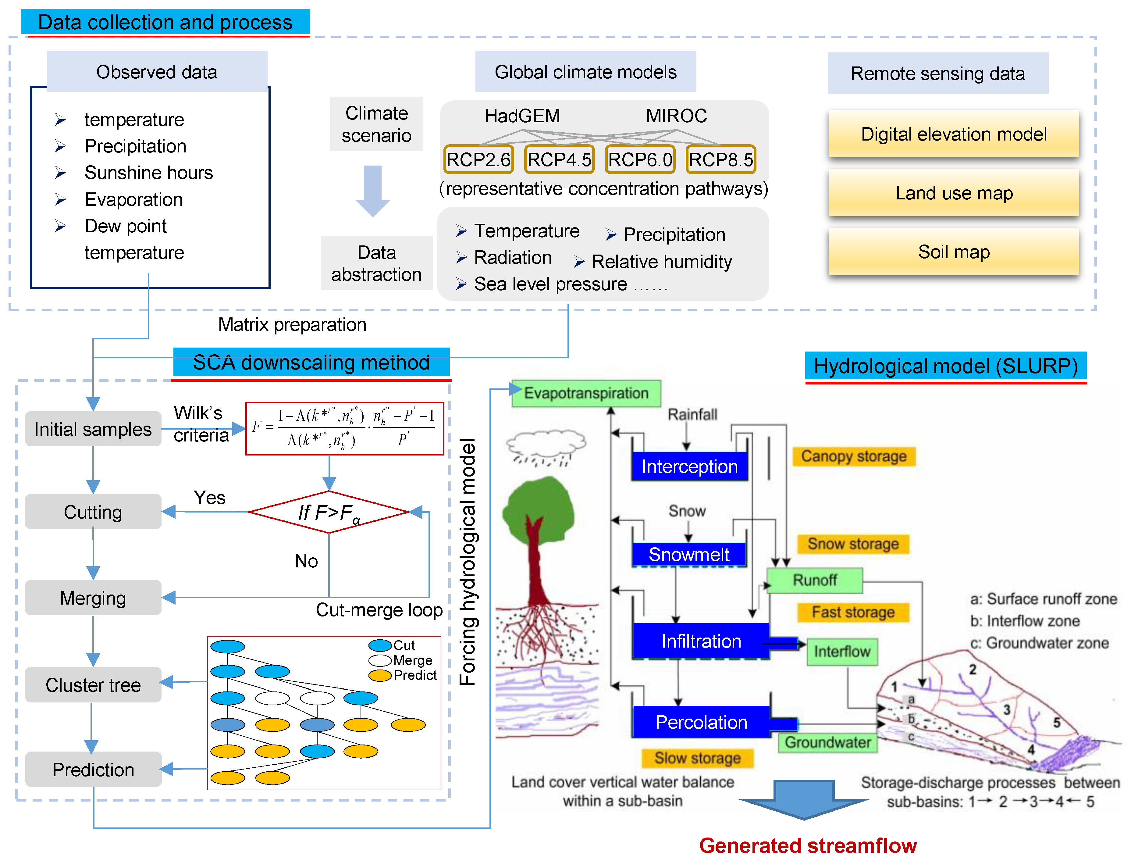
In this study, an ECHMS was developed and applied to Kaidu watershed. The detailed framework of ECHMS is displayed in
Figure 1. In ECHMS, eight climate scenarios (two GCMs and four representative concentration pathways (RCPs)) are set for gaining future climate change data and reflecting the uncertainties in climate models caused by physical mechanisms and human activities. The stepwise cluster analysis technique is applied to downscaling raw GCMs into site-scale, and then the downscaled data (e.g., temperature and precipitation) can represent the possible climate variations of Kaidu watershed. These climate data will be forced into calibrated SLURP model to generate future streamflow. Finally, future streamflow will be assessed to point out the characteristics of Kaidu watershed in the 21st century.
2.1. Problem Statement of Study Area
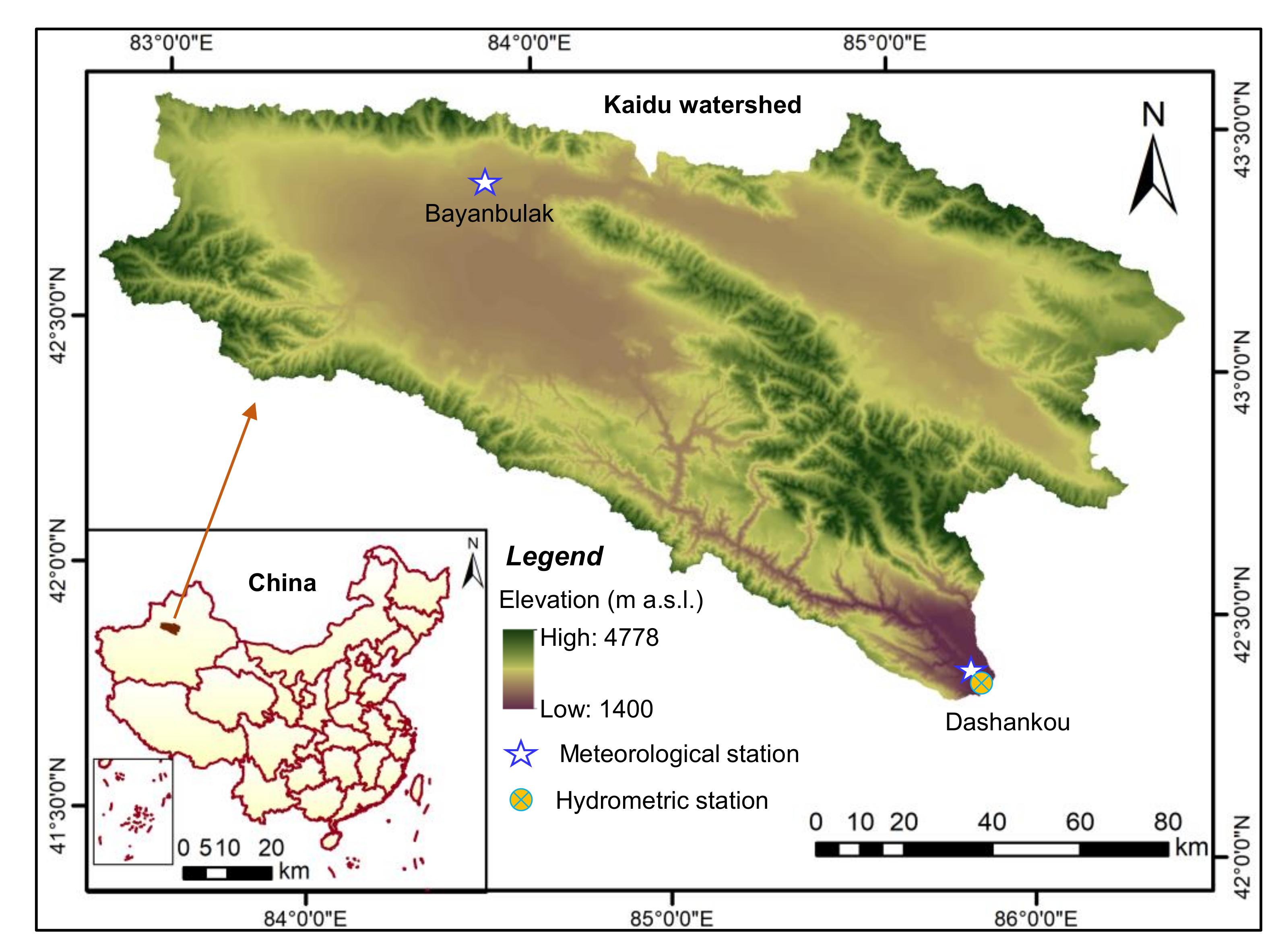
Kaidu watershed is a cold–arid region, located between 42°14′ N–43°21′ N and 82°58′ E–86°05′ E in northwest China (as shown in
Figure 2). The watershed covers an area of 18,827 km
2 with a large contrast in elevation (from 1400 to 4778 m a.s.l.). As recorded in the meteorological station of Bayanbulak (with an elevation of 2487 m a.s.l.), the annual temperature of this basin is −4.5 °C, and the minimum temperature is about −48.1 °C. It has an average annual pan evaporation of 1100 mm and precipitation of 262.6 mm [
24]. Due to the variation in elevation, this basin is characterized with strong gradients in both temperature and precipitation. The annual temperature and precipitation in Dashankou Station (with an elevation of 1400 m a.s.l.) are 7.5 °C and 99.6 mm, respectively. Besides, precipitation also varies with seasons and more than 80% of the annual precipitation occurs from May to September. The gross annual amount of surface water resources of the basin is approximately 3.3 × 10
9 m
3.
Due to climate change and human activities, the annual temperature and precipitation in Kaidu watershed has increased with decadal rates of 0.34 °C and 6.07 mm in the last century. If the increase in precipitation falls short of the temperature increase, evaporation may intensify and thus aggravate drought. Because the climate is an important driver of the hydrological cycle, the warming climate inevitably alters the distributions of water resources. In particular, temperature can directly affect glaciers, the most important source of water resources in Kaidu watershed, and thus can significantly affect the water resources and environmental conditions. Therefore, evaluating the future climate variation is very important for ecological environment and water resource management in Kaidu watershed.
2.2. Data Collection and Analysis
The datasets include (1) the GCMs used for climate projection, (2) the observed meteorological data used for both climate projection and hydrological model running, (3) spatial data for watershed delineation (i.e., DEM (digital elevation model) and land cover), and (4) hydrometric data for streamflow simulation. In detail, the GCMs (with periods of 1985–2000 and 2010–2099) used in this study were HadGEM and MIROC, under RCPs of 2.6, 4.5, 6.0 and 8.5, which were downloaded in the Coupled Model Inter-comparison Project (CMIP5) from the program for Climate Model Diagnosis and Inter-comparison (PCMDI) website (
http://www-pcmdi.llnl.gov). The predictors (including surface temperature, wind speed, surface upwelling longwave radiation, etc.) ranging from 1971–2000 were obtained from the National Centers for Environmental Prediction (NCEP) for SCA calibration and validation [
21]. DEM with resolution of 90 m are obtained from the Geospatial Data Cloud Website (
http://www.gscloud.cn). Land cover types in the year 2000 were prepared by the Resource and Environmental Sciences Data Centre Chinese Academy of Sciences (
http://www.resdc.cn). Meteorological data ranging from 1971–2010 (including daily temperature, precipitation, wind speed, and sunshine hours) were obtained from two stations (i.e., Bayanbulak and Danshankou). Due to the spatial heterogeneity of temperature and precipitation, the temperature input for elevation differences is derived with a lapse rate of 0.75 °C per 100 m, and precipitation is increased by 1% per 100 m based on the data obtained from the monitoring stations [
25]. The streamflow data (from 1971 to 2010) for the watershed were collected from Dashankou hydrometric station.
2.3. Stepwise Cluster Analysis
SCA is an efficient statistical tool that can establish the relationship between the predictors and predictands. It can deal with both continuous and discrete variables, as well as the nonlinear relationships between the variables. It divides the sample sets of predictors (i.e., the data from NCEP) and independent variables (i.e., temperature and precipitation) into different subsets (or sub clusters) through a series of cutting and merging operations [
22]. The processes of SCA for climate downscaling can be divided into the following steps:
(1)
Establishment of cluster principles, the criteria for the cut and merge operation are based on Wilk’s statistic. According to Wilk’s likelihood ratio criterion, if the cutting point is optimal, the value of Wilk’s (
) should be the minimum, where
W and
H are the within and between the groups’ matrix, respectively [
26].
(2) Tests of optimal cutting points Assuming the optimal cutting point of cluster h is , and the relevant value of temperature or precipitation is ., then the F-test can be undertaken. If is satisfied, then cluster h can be cut into two sub-clusters according to the distribution of .
(3) Mergence of clusters. The judging criterion is also based on the F-value of two sub-clusters. In this procedure, only the dependent variable values of observed temperature or precipitation in the two sub-clusters are useful. If is satisfied, clusters e and f can be merged into a new cluster h.
(4)
Prediction. After all the calculations and tests have been completed when all the hypotheses of further cut or mergence are rejected, a cluster tree can be derived for each dependent variable. Then, the predictors derived from the GCMs will be forced into the cluster tree, and the predicted dependent variables (i.e., temperature and precipitation) can be obtained (i.e.,
,
is the mean of dependent variable
i in sub-cluster
) [
14].
2.4. SLURP Hydrological Model
The hydrological model used in this study was SLURP, which is a continuous, spatially distributed basin model to simulate the hydrological cycle from precipitation to runoff [
27]. A watershed is divided into several aggregated simulation areas (ASAs) based on DEM maps through Topographic Parameterization (TOPAZ). SLURP conceptualizes each ASA into four storage tanks (canopy storage, snow storage, fast storage and slow storage), representing canopy interception, snowpack, aerated soil storage and groundwater, respectively [
28]. SLURP conducts a vertical water balance based on each of the land covers in the ASAs at a daily time step. At each time step, the model is applied sequentially to a matrix of ASAs and land covers. Each ASA must contribute runoff to an identifiable stream channel, which is connected to the watershed outlet.
In this study, the Kaidu watershed is divided into 183 ASAs. The weather data of each ASA (i.e., precipitation, temperature, dewpoint temperature, global radiation) is calculated based on local weather station using the Thiessen polygon method. In each ASA, precipitation is intercepted by the canopy or evapotranspiration, and any excess falls to the ground or to a snowpack depending on the air temperature. The evapotranspiration of the rainfall is calculated using the Penman–Monteith method of the Food and Agriculture Organization (FAO) [
29]. If a snowpack exists and the temperature exceeds a critical value, the snowmelt is computed using a simple degree-day method. Rainfall and any snowmelt infiltrate through the soil surface into the fast store depending on the current infiltration rate. If the precipitation factor exceeds the maximum possible infiltration rate, the surface runoff is generated. Runoffs are accumulated from each land cover within an ASA using a time/contributing area relationship for each land cover type [
24,
27,
30]. Manning’s equation is used to compute travel times for each land cover and estimate the velocities for travel both up-stream and down-stream. Then, the combined runoffs route to the next sub-basin in the way of hydrological storage routing
,
Q (m
3/s) is the outflow,
R is the combined runoffs routed into the channel in the sub-basin,
α and
β are the parameters specified to give the degrees of lag and attenuation required.
Before future projection, the model is calibrated and verified using observed data. The calibration of SLURP is conducted during 1971–1995 by an automatic method using the Shuffle Complex Evaluation algorithm developed at the University of Arizona [
31]. Then, the model was validated during the period 1996–2010 using the values of calibrated parameters. Nash–Sutcliffe efficiency (NSE), coefficient of determination (R
2), and the deviation of volume (DV) were used to address the goodness of fit of the performance of the hydrological model. The validated results can be found in Sun et al. [
2], which shows that the model is suitable for future projections. Then, the projected future temperature, precipitation, sunshine hours, and solar radiative are forced into the validated model for streamflow predictions.
3. Results and Discussion
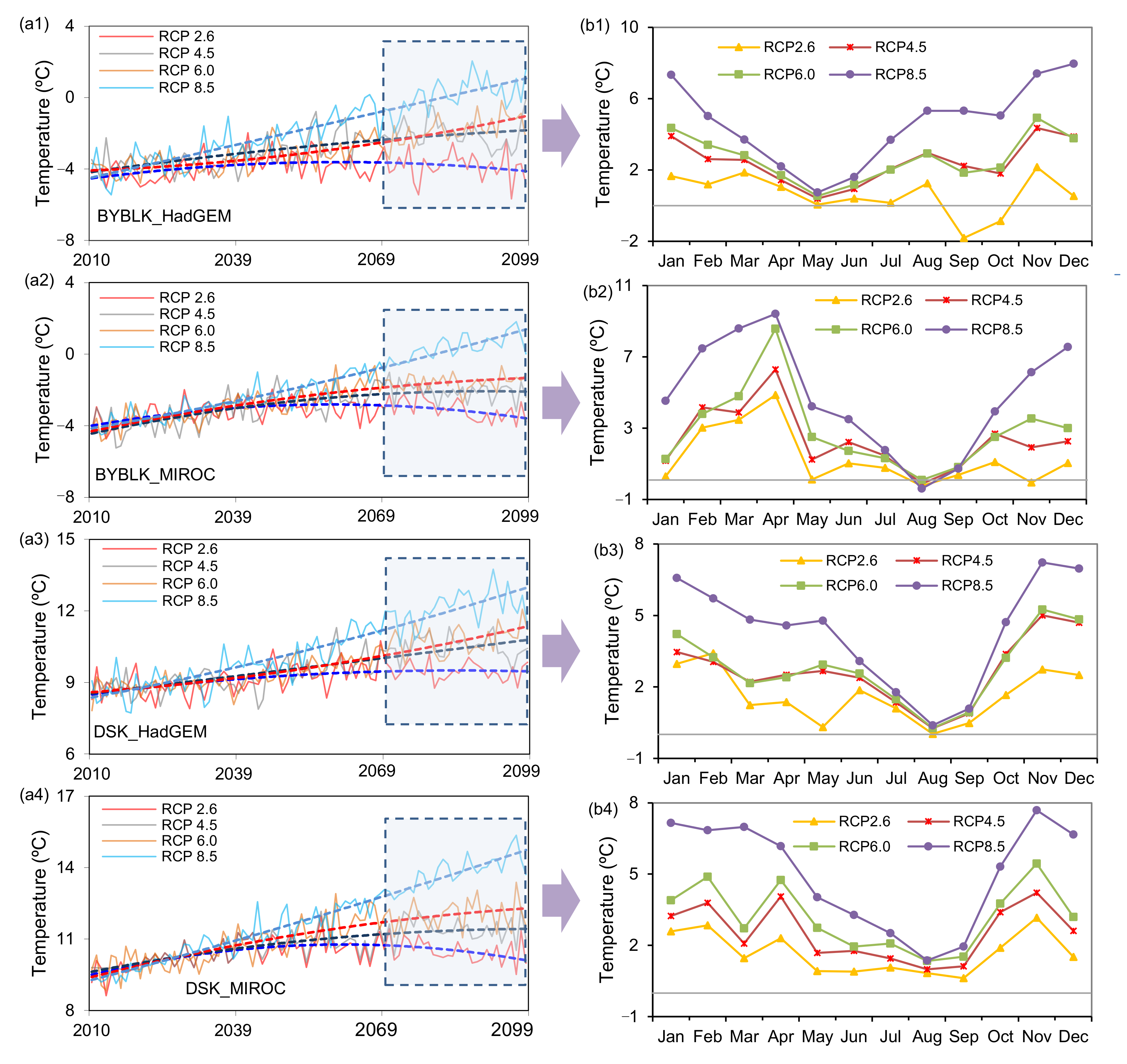
Figure 3 shows the temperature changes from 2010 to 2099. Results show that different climate scenarios would result in various annual/monthly temperature projections. By the end of the 21st century, Dashankou’s temperature would increase by 0.60–0.98 °C (RCP2.6), 2.3–2.8 °C (RCP4.5) and 2.4–3.0 °C (RCP6.0), and 4.6–5.3 °C (RCP8.5); Bayanbulak’s temperature would increase by 0.40–0.42 °C (RCP2.6), 2.3–3.1 °C (RCP4.5) and 1.8–2.9 °C (RCP6.0) and 5.4–5.6 °C (RCP8.5), respectively. The differences in temperature are mainly attributed to the varied physical mechanisms and conditions of climate models and RCPs. From the perspective of RCPs, temperature increment is the largest under RCP 8.5 and the smallest under RCP 2.6. This is due to the fact that RCP8.5 is a non-climate-policy scenario, resulting in severe changes in climate and RCP2.6 represents a rigorous climate policy, mostly to limit greenhouse gas emissions and, accordingly, low climate change impacts. The greenhouse emission scenarios under RCP 4.5 and RCP 6.0 are similar to the current situation, which means that if current industrial activities remain unchanged, future temperature would increase by nearly 3 °C. From the time-scale, temperature difference among the four RCPs is weak in the early 21st century and gradually increases with time. As shown
Figure 3b, the monthly temperature changes in the 2080s reveal that the temperature in July and August (summer) do not change much. In November, December, January, February, March and April, the temperature changes are relatively large. For example, in Dashankou, the temperature increases in December are 4.69 °C (RCP4.5 of HadGEM). The results suggest that the warming in the Kaidu watershed is mainly contributed by the warming in winter and spring, resulting in a smaller temperature difference during the year. As a result, the duration of summer may increase, and the winter may become shorter.
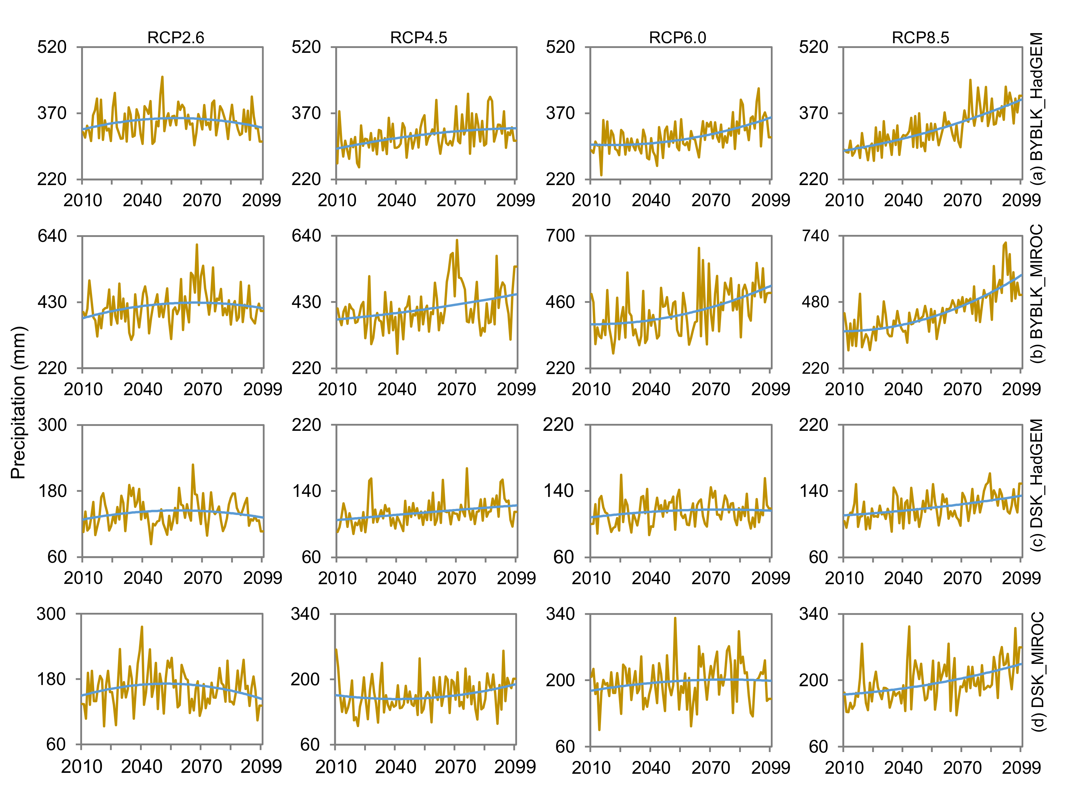
Figure 4 depicts the estimated annual precipitation in all scenarios. The results show that the precipitation shows an overall upward trend. By the end of the 21st century, the decadal precipitation in Bayanbulak increases by approximately 0.8–4.2 mm (RCP2.6), 3.4–5.6 mm (RCP4.5), 7.1–15.5 mm (RCP6.0) and 12.7–24.6 mm (RCP8.5); the precipitation in Dashankou increases by about 0.4–0.8 mm (RCP2.6), 2.2–2.8 mm (RCP4.5), 0.9–2.6 mm (RCP6.0) and 2.5–6.8 mm (RCP8.5). It shows that precipitation variation in Bayanbulak is greater than that in Dashankou. This is because Bayanbulak is located in a cold mountain area at high altitude, which is more sensitive to climate change. Besides, the projected precipitation under MIROC is higher than that under HadGEM. Annual precipitation in most years of the 21st century is about 150–300mm higher than the baseline under MIROC, and 50–150 mm higher than the baseline under HadGEM. This shows that different GCMs have a large amount of predicted precipitation due to the inconsistency of physical mechanisms and initial parameters. Besides, GCM’s ability to predict precipitation is still relatively poor, and there is a large deviation. The seasonal changes of precipitation summarized in
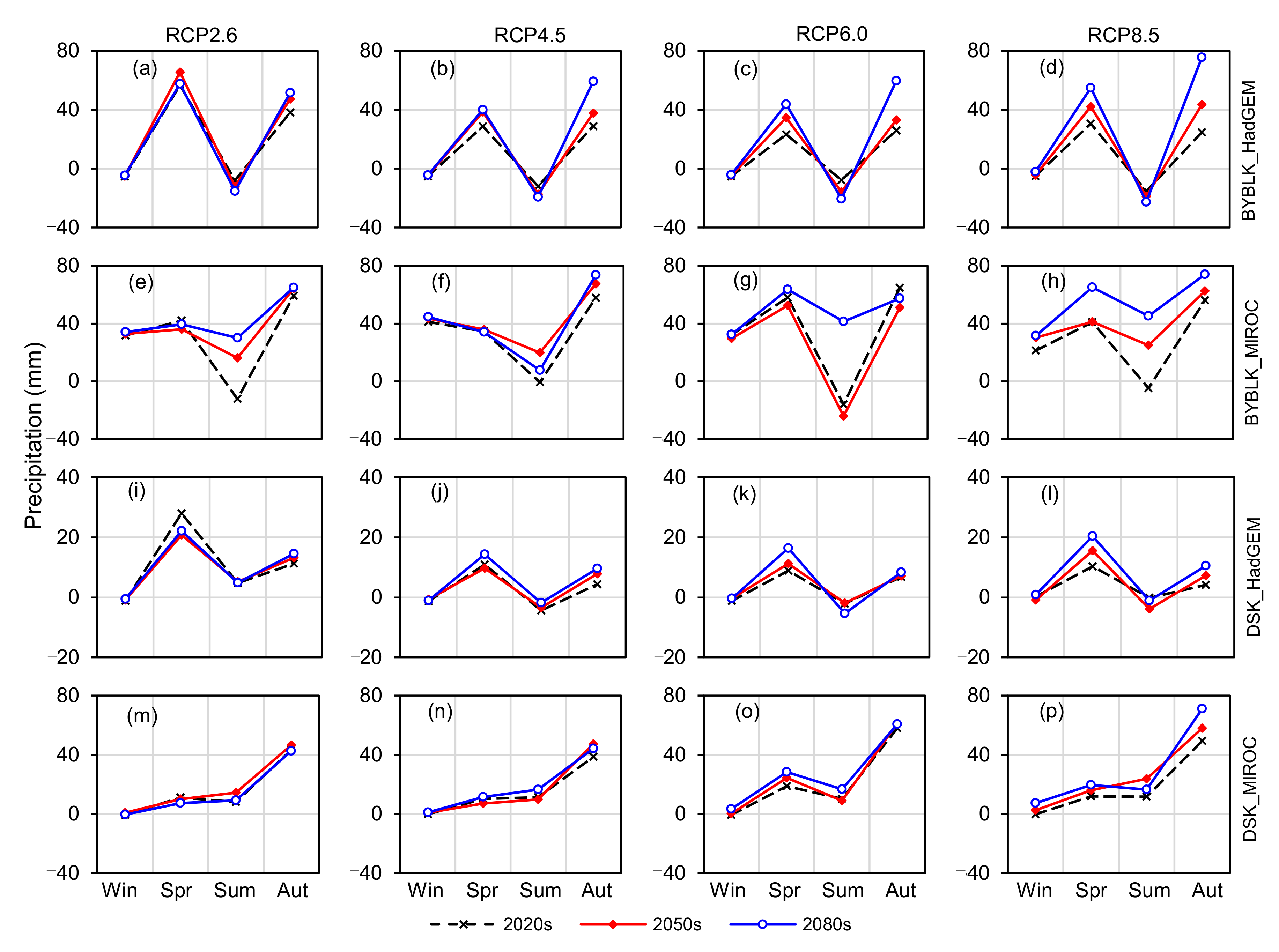
Figure 5 show that precipitation in spring and autumn in both stations would increase. However, the summer and winter precipitations present decreasing trends. This means that in the Kaidu watershed, abundant precipitation in spring and autumn would result in a balanced distribution of rainfall within the year. The decreasing winter precipitation indicate that winter will become more arid, and the possibility of seasonal drought time will increase.
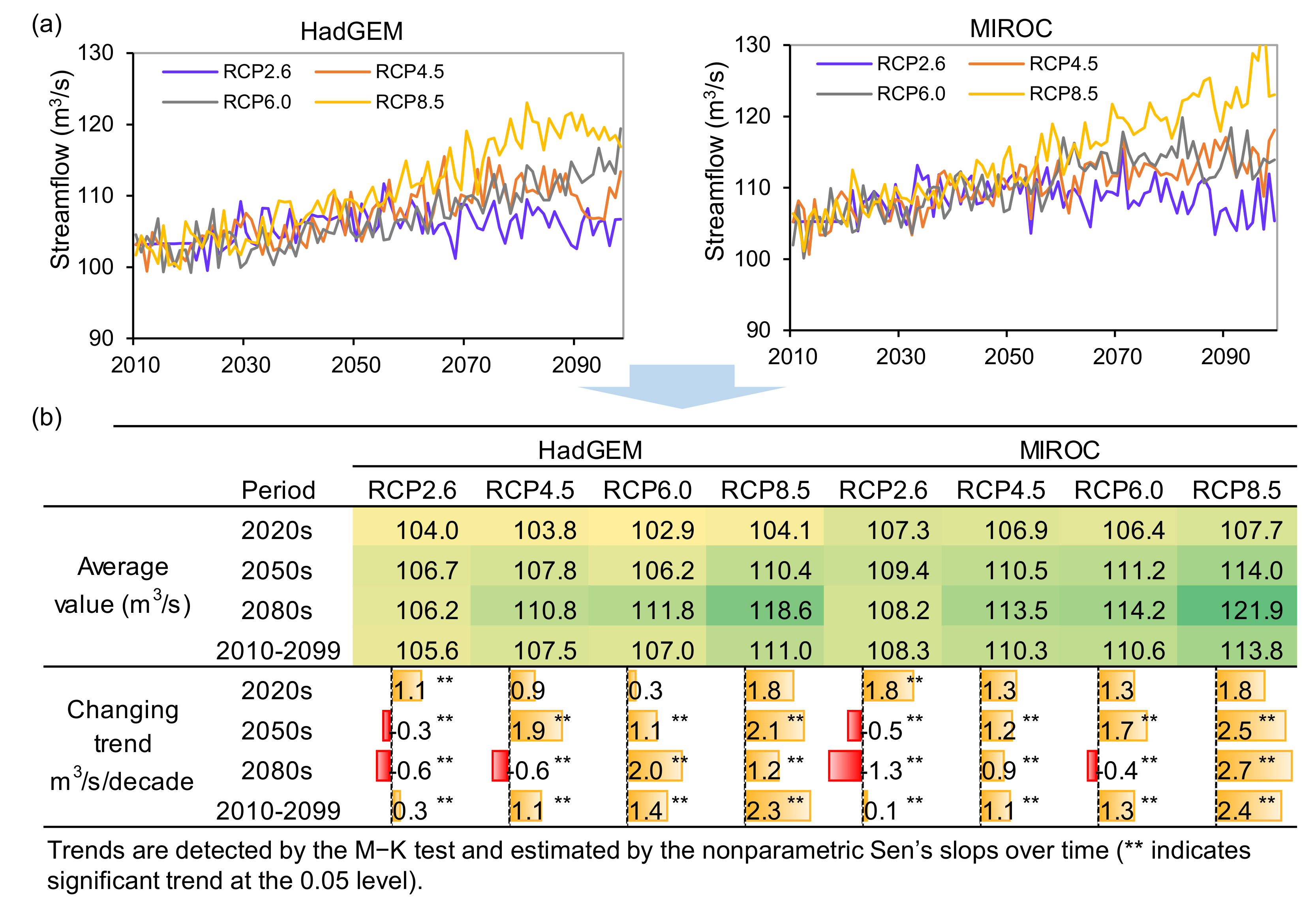
Figure 6 shows the predicted runoff of Kaidu watershed in 2010–2099. There are certain differences in the runoff across the eight scenarios. For example, under the HadGEM model, the average streamflow during the period 2010–2099 under the four RCP scenarios are 105.6 m
3/s (RCP2.6), 107.4 m
3/s (RCP4.5), 107.0 m
3/s (RCP6.0) and 111.1 m
3/s (RCP8.5), respectively. The average annual streamflow in the four RCP scenarios under the MIROC model are 108.3 m
3/s (RCP2.6), 110.3 m
3/s (RCP4.5), 110.6 m
3/s (RCP6.0) and 113.8 m
3/s (RCP8.5). In general, the streamflow in the RCP2.6 scenario is the least, and the streamflow in the MIROC model is higher than that in the HadGEM model, which is consistent with the changing trends of temperature and precipitation. By comparing various scenarios, the possible streamflow range of the Kaidu River in the future can be obtained, avoiding the errors caused by the prediction of a single scenario.
Mann–Kendall (M–K) test was implemented to analyze the changing trend of annual streamflow in Kaidu watershed (as shown in
Figure 6b). The future streamflow has a significant increasing trend during the period 2010–2099. The maximum increasing rate is 2.4 m
3/s per decade under the RCP 8.5 of MIROC, and the minimum increasing rate is 0.1 m
3/s per decade under the RCP 2.6 of MIROC. However, by the middle or end of this century, the increase becomes unobvious, and even shows a downward trend. For example, under the RCP2.6 scenario, the projected streamflow would first remain flattened during the period 2010–2025. This trend may be due to an experiment error by the SCA method. In the downscaling process, SCA may dilute the peak values of climate variables, resulting the projected temperature and precipitation being downscaled into a cluster with similar values. Then, the streamflow would slightly increase before 2050s; after 2050s, a decreasing trend would be observed. Streamflow under RCP4.5 and RCP6.0 have a stabilized trend and then decline slightly after 2080; streamflow under RCP8.5 has an obvious increasing trend before 2090; after that, a slight downward trend would be observed. The increase in streamflow is contributed by increments in precipitation and temperature. Kaidu is a river that is supplied by precipitation and ice and snow streamflow, and the increase in temperature leads to an increase in snowmelt streamflow. The slight decrease in streamflow under RCP4.5 and RCP6.0 around 2080 is caused by precipitation and temperature. In these two scenarios, the precipitation increased slightly, and the temperature shows a steady state and is about 2 °C higher than the current temperature. The increase in temperature also leads to increased evaporation, which caused a slight decrease in the streamflow. The downward trend of streamflow in the RCP8.5 scenario is determined by temperature. This is because the precipitation in this scenario is increased, and the temperature is 4 to 5 °C higher than the baseline. The evaporation is very large, far exceeding the precipitation, which would lead to a decrease in streamflow.
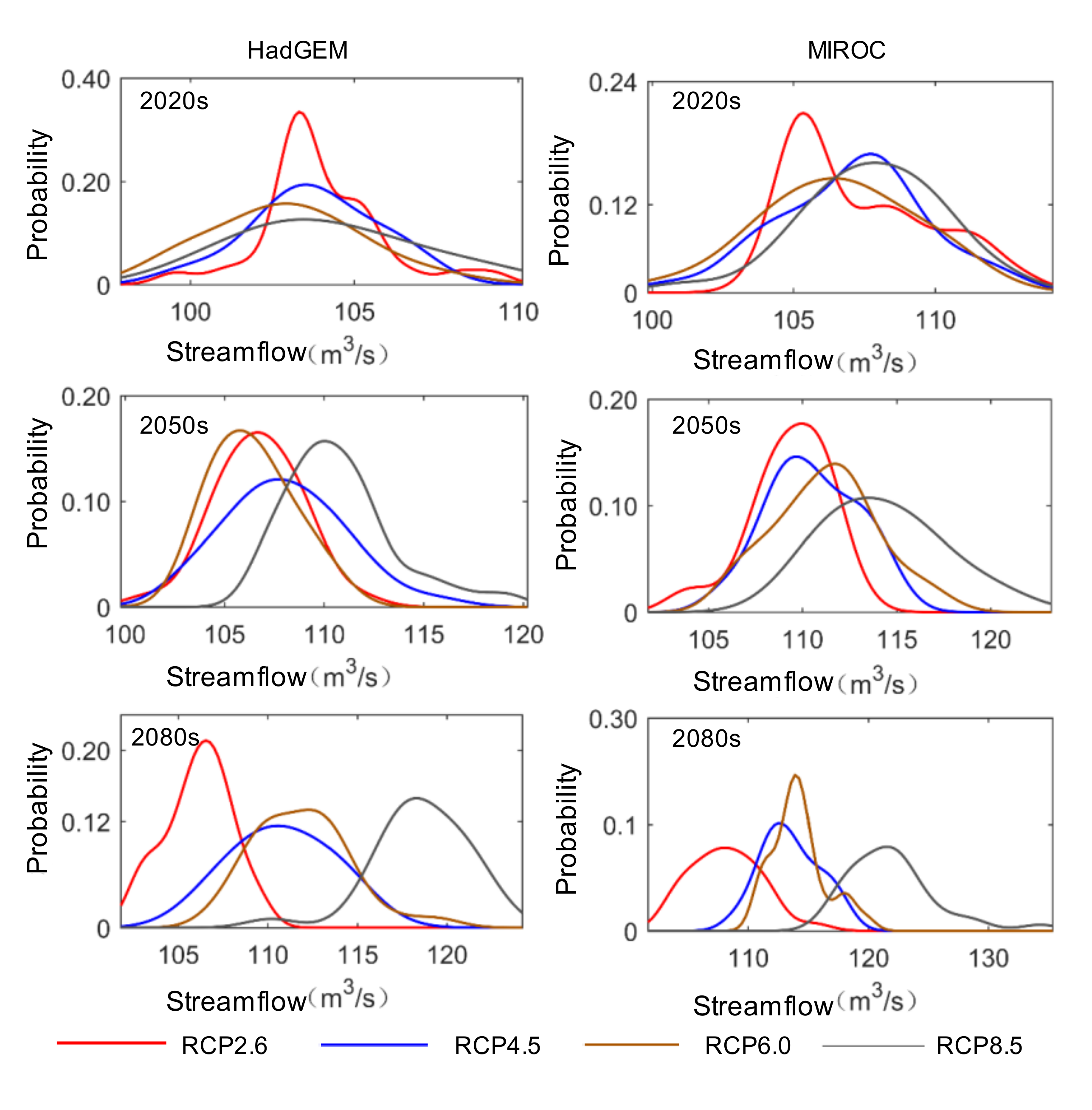
Figure 7 presents the annual streamflow distribution during the 2020s, 2050s and 2080s. Results show that the difference in streamflow among the RCPs in the 2020s is the smallest, followed by the 2050s and 2080s. For example, in the 2020s, the average streamflow under HadGEM is around 103 m
3/s, while in the 2080s, the average streamflow fluctuates between 106.2 and 121.9m
3/s. Such deviation is similar with those of temperature and precipitation. These results suggest that uncertainty in different climate scenarios exists, and it would be amplified along with time.
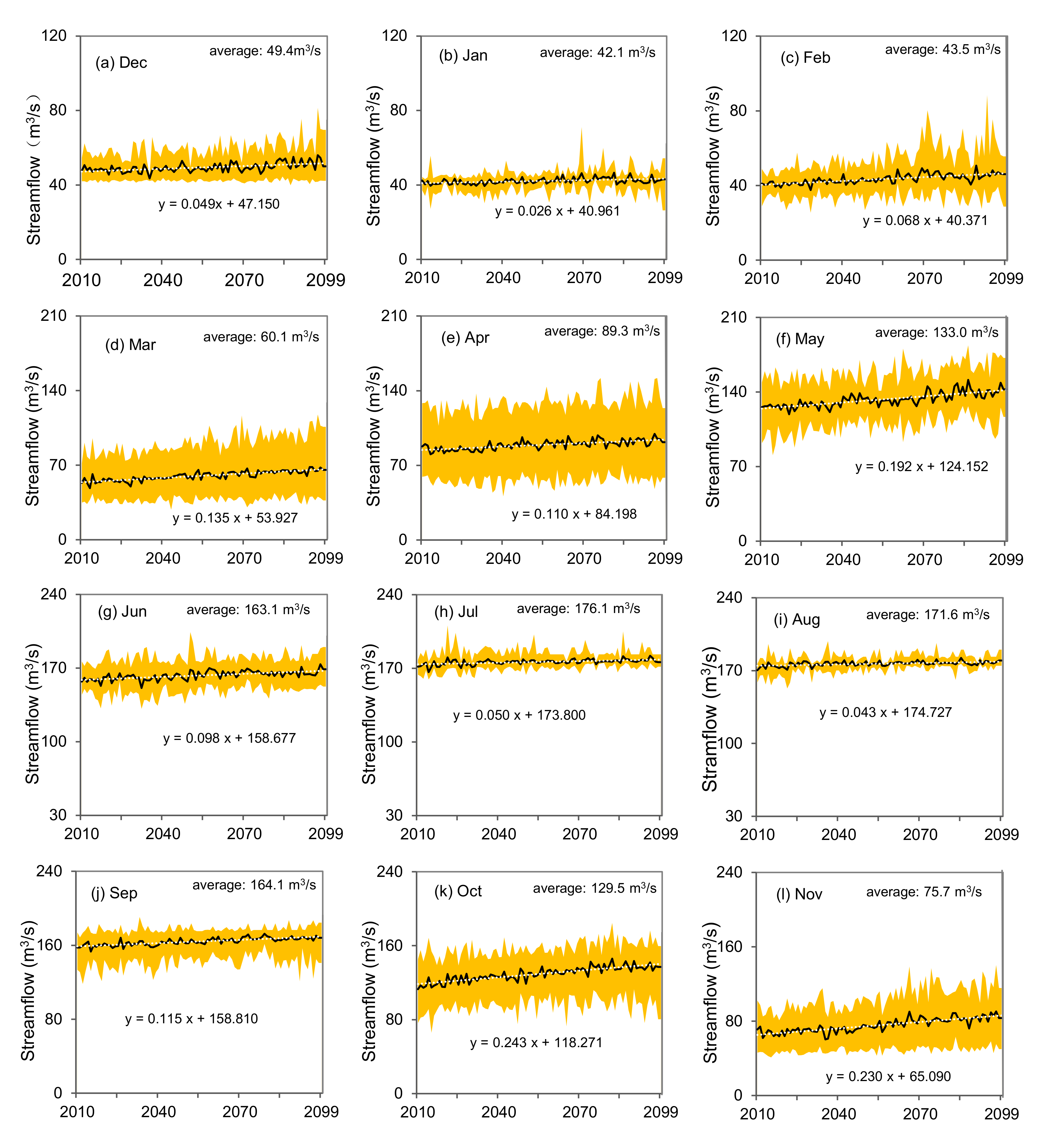
Figure 8 describes the changes in streamflow in different months. January has the lowest average multi-year monthly streamflow (42.1 m
3/s) and July has the highest one (176.1 m
3/s). Besides, the streamflow in all months shows overall increasing trends. The largest increasing rate is 2.43 m
3/s in October and the smallest increasing rate is 0.26 m
3/s in January. In general, the increasing rate is high in autumn and spring, and is low in wither and summer, illustrating that the annual streamflow increment is mainly attributed to autumn and spring. Results also show that the ranges of streamflow change in July and August is relatively small. This not only shows the accuracy of climate prediction for summer streamflow, but also shows that the response of summer streamflow change to climate change is relatively stable. However, the results of spring (March, April and May) show a great difference among scenarios. For example, in April, the multi-year average of the minimum predicted streamflow in all scenarios is 58.2 m
3/s, while the multi-year average of the maximum is 128.3 m
3/s, with a difference of up to 120%. This illustrates that the spring streamflow is more sensitive to climate change. This may be due to the complexity of streamflow generation in spring. The Kaidu river is supplied by snowmelt and precipitation streamflow, so there will be two peaks of streamflow in a year, respectively, in spring and summer. Due to the combined influence of snow depth and temperature, snowmelt streamflow is more complicated than precipitation streamflow. Therefore, there is a large uncertainty in the interpretation of snowmelt streamflow in different climate scenarios.
4. Conclusions
In this study, an ECHMS has been developed for assessing the streamflow in Kaidu watershed. The ECHMS consists of multiple climate change scenarios, the SCA and the SLURP model. The modeling system not only reflects the uncertainty in climate models caused by heterogeneity in physical mechanism and initial parameters, but also reflects the uncertain information caused by greenhouse gas emissions. The SCA downscaling method can effectively handle the complex non-linear and discrete relationships between climate elements and overcome the functional hypothesis of conventional statistical methods. The SLURP model is a semi-distributed physical model that can effectively model streamflow processes by snowmelt and rainfall with simplicity of operation.
Results show that by 2099, the temperature in the Kaidu watershed will increase, with the RCP8.5 scenario having the largest increase, reaching more than 5 °C. Annual warming is mainly contributed by the warming in winter and spring, resulting in a smaller temperature difference during the year. This may increase summer duration and shorten winter duration. By the end of this century, the precipitation shows an increasing trend. Precipitation in spring and autumn will increase more obviously, resulting in the difference in precipitation between spring, summer and autumn. As a result, the distribution of rainfall within the year will be balanced. The precipitation in winter has a decreasing trend, indicating that winter will become more arid. In the future, there is an overall increasing trend of streamflow with a range from 105.6 to 113.8 m3/s. The increasing rate is high in autumn and spring and is low in winter and summer. The maximum average increasing rate is 2.43 m3/s per decade in October and the minimum is 0.26 m3/s per decade in January. This illustrates that the annual streamflow increment is mainly attributed to autumn and spring. Summer streamflow response to climate change is relatively stable, while spring streamflow change is more sensitive to climate change.
Through the above results, the temperature, precipitation and streamflow of Kaidu watershed in 2010–2099 were identified, which is beneficial for local water management. However, there are still some limitations in this study. For example, there are many GCMs developed by many institutes; however, only two GCMs are explored in this study to explore their uncertainties. This may be not enough to provide more accurate projection results. Thus, more GCMs and ensemble outputs of them should be adopted in future studies. Besides, this study focuses on a data-scarce region with only two meteorological stations. This may dilute the heterogeneity in climate features in the large watershed and bring errors in streamflow prediction. In future studies, multiple-source meteorological data (e.g., reanalysis data and remoting data) are suggested to capture higher-resolution climatic and hydrological characteristics.


