Evaluation of the Main Function of Low Impact Development Based on Rainfall Events

Abstract

Low Impact Development (LID) is one of the sustainable approaches to urban stormwater management in areas with rapid urbanization. Although LID has been shown to have a positive effect in flood reduction, the hydrological balance regulation effect of LID under a variety of rainfall events is not fully understood. In this study, we assessed the hydrological efficiency of LID at two residential–commercial mixed sites in Korea to investigate the main function of LID in terms of diverse rainfall characteristics. Storm Water Management Model (SWMM) was constructed to simulate the hydrological process numerical simulations in the pre-development, post-development and LID design scenarios, respectively. The model was calibrated and validated by using five observed rainfall–runoff events. Then, four single and four multiple LID practices (LIDs) were used to estimate their effectiveness under seven different designed rainfall events. The results indicate that LIDs substantially influence the hydrology cycle system, while the regulating effect varies with rainfall amounts. The efficiency of LIDs in flood reduction is proved to be more effective during lower storm events. However, LIDs should be designed to primarily prioritize the restoration of hydrological balance when the rainfall return period is longer.

1. Introduction

Rapid urbanization is one of the most significant trends in the twenty-first century, causing a series of new challenges on the hydrological cycle, such as increasing impervious areas and increasing rainfall intensity [1,2]. Increased impervious area intercepts rainwater seeping into the soil layer, thereby leading to a marked increase in surface runoff and the reduction of groundwater recharge [3,4]. In addition, as an increasing number of people migrate to urban areas, the resulting increase in population density has affected the regional climatic characteristics of urban areas, leading to a high frequency of extreme weather events [5].

Under dual pressure from urbanization and extreme rainfall, the efficient drainage network system is proposed as a strategy to accelerate rainwater drainage from the urban area [2]. However, the conventional drainage system is mainly focused on rainwater quantity control, while other vital aspects, such as water quality, groundwater protection and water cyclic utilization, are ignored. Recently, many urban stormwater managers increasingly realize the limitations of the traditional drainage system; thus, more sustainable drainage systems have been established for urban stormwater management. Low impact development (LID) proposed by the United States is an environmental stormwater management approach, which particularly emphasizes the decentralized microscale control measures at source by using techniques that perform penetration, retention, storage and purification functions to restore the deteriorated hydrological conditions to a nearly pre-development state [6,7]. Therefore, an urban stormwater system based on LID could not only alleviate the flood disaster caused by rainfall runoff but also adequately utilize urban rainwater resources, which meets the sustainable requirements of urban stormwater management.

LIDs have been demonstrated to control rainwater quantity, improve water quality, restore the water cycle and protect the ecosystems. For instance, Li et al. [8] used SUSTAIN to evaluate the performance of LIDs at a residential–educational mixed zone in Shenyang, China, and indicated that LIDs could effectively reduce annual runoff volumes and pollutant loads. Lee [9] assessed the efficiency of LIDs at a residential site in Korea and confirmed the positive effects of LIDs in water cycle restoration. Martin-Miklea et al. [10] introduced a spatially explicit approach to identify LID priority sites at a mixed-use region in central Oklahoma, US, and revealed that LID can diminish the negative effects of urbanization on stream ecosystems.

On the other hand, although the positive effects in the hydrological performance of LIDs have been verified, many scholars reported that the effectiveness of LIDs could vary depending on regional characteristics. For example, Goncalves et al. [11] presented the runoff reduction between 30% and 75% could be achieved for seven different designed LID scenarios correspondingly. The various combinations of LIDs having a different impact on hydrology performance and water quality were suggested by Liu et al. [3] and Li et al. [8]. Wu et al. [12] presented that the increase in the implementation area with LIDs does not necessarily mean more efficient flow reduction. Additionally, Luan et al. [13] have focused on the simulation of LID in a mountainous low-lying urban region and concluded that, in contrast to the plain urban zone, there might be high risks of flooding and waterlogging in a mountainous urban zone. Gilroy et al. [14] utilized a spatial-temporal model to determine the effects of BMPs on single-family, townhome and commercial lots, and the different effectiveness of BMPs was represented in response to different types of land use. Kong et al. [15] examined the hydrological features of the four urban development designed scenarios and implied that the LIDs take some roles in providing flood reduction in post-development urbanized scenario. Seo et al. [4] explored the performance of LIDs under three types of urban forms using SWAT, and their results show relatively lower effectiveness in the compact high-density urban land use. In addition to LID forms and land use types, rainfall characteristics could be another factor that influence the effectiveness of LIDs. For example, Goncalves et al. [11], Zhu and Chen [16] and Qin et al. [17] represented the LID efficiency highly depends on the duration or intensity and the pattern of the rainfall. Luan et al. [13] and Qin et al. [17] revealed the LIDs are more effective in flood reduction during heavier and shorter storm events. However, most studies have focused on the effectiveness in flood reduction of LIDs under different rainfall characteristics, and an evaluation of the hydrological balance regulation effect of LIDs under a variety of rainfall amounts has not been performed.

Therefore, SWMM was constructed as a modeling tool to simulate the hydrological process in two case study regions, and these numerical simulations were performed under different land use types (in the pre-development, post-development and LID design scenarios). The main objective of this study was to assess the hydrological benefits of LIDs in the urban areas for exploring the variations in hydrological elements after LID implementation to identify the primary function of LIDs under different rainfall characteristics. To this end, this study examined the variations in hydrologic components to estimate the effect of LIDs in the hydrological cycle balance and runoff reduction under seven design rainfall amounts. Meanwhile, LID practices, including rain garden (RG), pervious pavement (PP), rain barrel (RB) and vegetative swale (VS), were used to compose four single and four multiple LIDs. Our work clarifies the main function of LIDs under different rainfall characteristics and can assist in decision-making in future urban planning.

2. Materials and Methods

2.1. Study Area Description

The case study areas were the Gwanpyeong region and the Munji region, which are located in Yuseong-gu, Daejeon city, South Korea (Figure 1). The city of Daejeon, which has a population of over 1.51 million, is the fifth-largest metropolis of South Korea. The Gap creek, as one of the important tributaries of the Geum River, is originated from Daedun Mountain, flows through the Daejeon city and finally joins the left bank of the Geum River. The climate of Daejeon is influenced by the monsoon, and the monthly mean temperature ranges from −1.0 °C in January to 25.6 °C in August. The annual average precipitation is about 1458.7 mm and mainly concentrates in summer. In addition, one weather station and three gauging stations nearby the Gap creek can automatically measure meteorological and hydrological data.

This study covered two typical residential–commercial mixed areas, which have different drainage ratios of conduits (Figure 2). The drainage ratios of conduits could signify the amount of total rainfall volume draining out through the drainage pipes, which means the drainage capacity of conduits in the two areas under the same rainfall condition. The CAD data used in this study come from Daejeon city hall and a previous study in Gwanpyeong [18]. The Gwanpyeong region is located downstream of the Gwanpyeong creek, which is a tributary of the Gap creek. The area is 63.1 ha, and the precipitation drains into the Gwanpyeong creek through the northeastern outfall. The Gwanpyeong region is a developed residential–commercial mixed region with a lower drainage volume ratio of conduits. The residential zone consisting of apartment and villa has the highest proportion at 40%, and the impervious area including parking lots and roads occupies the second place at 25.8%. Comparatively, the grassy area had the lowest proportion at 13.6%, while the proportion of commercial business district and the public place (20.1%) is slightly higher than that of the grassy area. In addition, the main stream of the Gap creek flows through on the right of the Munji region where the area is 30.1 ha, and the effective rainfall collected in the region flows into the Gap creek through two drainage outlets in the northeast and southeast corner. The Munji region is a newly developing residential–commercial mixed region with a relatively higher drainage volume ratio of conduits. The proportion of residential zone in the Munji region is 40%, while the impervious area is as high as 29.6%. In the meantime, 19.3% is composed of the commercial district, and the grassy area has the lowest percentage of approximately 6.2%.

2.2. SWMM

Computer models such as L-THIA-LID 2.1 [3], SWAT [4], SWMM [13] and SUSTAIN [19] have been used to objectively evaluate the effectiveness of LID practices (LIDs). Among them, EPA Storm Water Management Model (SWMM) is a dynamic rainfall–runoff simulation model using a single or long-term event to predict the runoff and pollutant loads in urban areas, which has been widely used for the simulation of LIDs [20,21]. The latest version of SWMM is version 5.1.014 released in February 2020, which provides an integrated environment for editing input data and then running hydrological, hydraulic and water quality simulations. Furthermore, the results could be expressed in a variety of formats, including color-coded drainage area, time series graphs and tables, profile plots and statistical frequency analysis [21]. Therefore, SWMM was selected as the simulation model in this study.

The hydrological cycle demonstrates many interconnected components, including precipitation, evaporation, infiltration, depression storage and runoff. In this study, design rainfall and annual average evaporation were used to simulate precipitation and evaporation. The Green–Ampt method, as an infiltration function, is suitable for a relatively small-scale area, takes into account the soil characteristics of the study area [22] and can be calculated by Equation (1). After the infiltration process, the effective rainfall would flow into the drainage network system to finally get the outflow in each sub-catchment. SWMM estimates a quantity of surface runoff in response to a rainfall event using nonlinear reservoir routing of overland flow, which is calculated by the continuity equation (Equation (2)) and Manning’s equation (Equation (3)). In addition, flow routing within a drainage network system can be calculated by the one-dimensional Saint–Venant equation [21]. In this study, we employed the dynamic wave routing, which is suitable to reproduce the overflow from the urban drainage network and the pressurized flow in the closed conduits, and assessed the flow in conduit by the continuity equation (Equation (2)) and momentum equation (Equation (4)):

$$F=\frac{K_s{S}_w\left({\theta }_s-{\theta }_i\right)}{i-K_s}$$

(1)

where F is the infiltration ($mm$), ${\theta }_s$ and ${\theta }_i$ are the saturated and initial moisture content, i is the rainfall intensity ($mm/h$), $K_s$ is the saturated hydraulic conductivity ($mm/h$) and $S_w$ is the soil capillary suction at wetting the front ($mm$).

$$\frac{\partial Q}{\partial x}+\frac{\partial A}{\partial t}=0$$

(2)

$$Q=W\frac{c}{n}{\left(d-d_s\right)}^{5/3}{S}^{1/2}$$

(3)

$$\frac{1}{gA}\frac{\partial Q}{\partial t}+\frac{1}{gA}\frac{\partial }{\partial x}\left(\beta \frac{Q^2}{A}\right)+\frac{\partial h}{\partial x}-S_o+S_f=0$$

(4)

where $Q$ is the discharge ($m^3/s$), $\mathrm{A}$ is the cross-sectional area ($m^2$), $W$ is the width of the sub-catchment ($mm$), $S$ is the slope of the sub-catchment, $c$ is a constant, $n$ is Manning’s coefficient, $d$ is the water depth ($mm$), $d_s$ is the depression depth ($mm$), $h$ is the pipe water depth ($m$), $t$ is the time ($s$), $x$ is the distance, $S_f$ is the friction slope and $S_o$ is the bottom slope.

2.3. Simulation Scenarios

The three scenarios were designed based on the type of land use, including the pre-development, post-development and LID design scenarios. Among them, the pre-development scenario assumes that the catchment has the same conditions as those before urbanization. Considering the different times of concentration, two assumptions for the pre-development scenario exist: the drainage pipe network is established in the same state as itself after development to ensure the same sub-catchment case and the condition of land use in pre-development is regarded as green space. In addition, the post-development scenario represents the existing situation after urbanization in which the LIDs have not been designed. It is the baseline for assessing the runoff performance of the LIDs. Besides, the LID design scenario signifies that the LIDs have been implemented based on the post-development scenario. Considering the feasibility and convenience of installation, RG, PP, RB and VS were combined in various ways to compose four single LIDs and four multiple LIDs (

Table 1. Design area of LIDs in the study area.

LID Scenarios		Gwanpyeong Region	Munji Region
S-RG	S-RG	16.5%	9.1%
S-PP	S-PP	21.3%	13.3%
S-RB	S-RB	349 (number)	197 (number)
S-VS	S-VS	5.3%	7.1%
RG + PP + RB + VS	M-LID1	43.1% 1	29.4% 1
50% PP + RB + RG	M-LID2	27.1% 1	15.7% 1
50% PP + RG + VS	M-LID3	32.4%	22.8%
50% PP + RB + VS	M-LID4	15.9% 1	13.8% 1

¹ Does not include the number of RB; (%), Percentage of total area; (number), the number of RB.

).

According to the guideline of the LID design manual [23], LIDs can be constructed adjacent to buildings or streets and integrated into parking lots or green gardens. The LIDs were installed on the available impervious areas by considering the land use data and the actual situation. Therefore, in this study, RGs were set in the park and large grassy areas to capture the runoff generated from the impervious surface around them. PPs were integrated into the parking lots and sidewalks to capture the runoff from the concrete surface around them, which were located in different sub-catchments. VSs were constructed on the small grassy area to handle the rainwater from the road. RBs were placed above the ground in an individual residential zone for capturing the rainwater from the roofs. These LIDs were installed in the available location to capture surface runoff and provide space for detention and infiltration to the hydrological cycle. The design area of each LID (Table 1) was obtained by reference to the actual available land obtained by measurements at Google Earth.

2.4. Design Rainfall

Due to the lasting effects of global climate change, the hydrological environment is subject to major changes in the next few decades. Even more extreme storm events are expected to frequently occur all over the world [24]. To cope with extreme rainstorm events, design rainfall, which is not observed but artificially generated, was selected for the rainfall–runoff simulations. The difference of rain pattern not only affects the time of peak rainfall but also leads to the difference of total runoff volume produced by rainfall in the basin. Therefore, the distribution of total rainfall should not be based solely on the typical rainfall process but should be studied and analyzed based on a large amount of local rainfall data, so as to select a suitable rainfall pattern. Temporal distribution methods of design rainfall include the Mononobe method, Huff method, Keifer and Chu method, Pilgrim and Cordery method, Yen and Chow method and alternating block method [25]. The representative distribution for generating design rainfall data in Korea is the Huff distribution, by which all drainage facilities in Korea are designed [26]. The general procedure of the design rainfall is summarized as follows: First, the observed rainfall data from 1969 to 2017 were collected from the Daejeon weather station. Second, the probability rainfall was calculated by return period and storm duration using Fard 2006, a frequency analysis software package, which is widely used in Korea [27]. The results are shown in

Table 2. Probability rainfall by duration and return period in Daejeon station (unit: mm).

Return Period	Storm Duration
	10 min	20 min	30 min	40 min	50 min	60 min	90 min	120 min
2 years	15.5	24.3	30.3	35.7	39.9	44.2	53.2	59.4
3 years	17.7	27.7	34.5	40.5	45.3	50.9	61.9	68.8
5 years	20.3	31.5	39.2	45.8	51.4	58.4	71.6	79.2
10 years	23.5	36.3	45.1	52.6	59	67.8	83.8	92.4
30 years	28.4	43.6	53.9	62.7	70.6	82	102.2	112.2
50 years	30.6	46.9	58	67.4	75.8	88.4	110.6	121.3
100 years	33.6	51.3	63.4	73.6	82.9	97.2	122	133.5

. It is worth noting that the probability rainfall under different return periods (T = 2, 3, 5, 10, 30, 50 and 100 years), and rainfall durations (10, 20, 30, 40, 50, 60, 90 and 120 min) were separately examined.

Then, the temporal distribution method was used to calculate the temporal distribution of the probability rainfall under different return periods and rainfall durations. The Huff method suggests nondimensional storm distribution patterns in which the rainfall distribution is divided into four distinct groups in terms of storm duration, and the peak rainfall intensity occurs in the first, second, third or fourth quarter of the storm duration. Generally, the third quartile in the Huff distribution has been considered to be appropriate for the design and operation of urban drainage facilities in Korea [26]. Equation (5) shows the cumulative regression equation of Huff method; the regression coefficients that are suitable for Daejeon use the constant of third quartile in the Huff distribution recommended by Korea Precipitation Frequency Data Server [28], which is an institution for flood forecasting and the operation of drainage facilities in Korea.

$$Y=C_0+C_{1}X+C_2{X}^2+C_3{X}^3+\cdots +C_n{X}^n$$

(5)

where $X$ is the dimensionless cumulative rainfall duration, $Y$ is the dimensionless cumulative rainfall and $C_i=0,1,2,\dots , n$ is the regression coefficient.

Finally, considering the probable maximum flood (PMF), different temporal distributions of probability rainfall were applied to the input parameters in SWMM to repeatedly simulate the hydrological process and predict the maximum discharge flow at two study regions. The results indicated that the maximum discharge flow appeared when the rainfall duration was 60 min in the two regions. Thus, the design rainfall duration of 60 min and the interval time of 6 min (Figure 3) were adopted to conduct hydrological simulations in this study for investigating the effectiveness of LIDs under the various return periods. The different return periods include 2, 3, 5, 10, 30, 50, and 100 years, which are represented by T = 2, 3, 5, 10, 30, 50 and 100 years, respectively. What should be highlighted here is the storm events adopted in this study have the same rainfall duration (60 min) and the same location of peak rainfall intensity (t = 42 min), and the corresponding total rainfall amounts range from 44.2 to 97.2 mm.

2.5. Input Parameters of SWMM-LIDs

SWMM parameters can be largely classified into hydrological and physical parameters [21]. Physical parameters, including sub-catchment area; slope and width, impervious areas; and length, diameter, and shapes of conduits, can be obtained from the Daejeon city hall, while hydrological parameters can be obtained from the manual or references. The relevant parameters of the Green–Ampt method are constant depending on the soil characteristics of the study area. Thus, we followed the recommended parameters [22], considering soil characteristics in Daejeon. The final value of conductivity was taken as 3.3 mm/h, suction head as 88.9 mm and initial deficit as 0.1. The other parameters shown in

Table 3. Main simulation options and parameters in SWMM.

Simulation Options	Unit	Value	Source
N-Impervious		0.015	Calibration and Validation
N-Pervious		0.55	Calibration and Validation
Pipe Roughness		0.013–0.015	Calibration and Validation
Dstore-Impervious	mm	1.35	Calibration and Validation
Dstore-Pervious	mm	1	Calibration and Validation
Soil Capillary Suction Head	mm	88.9	SWMM User Manual
Soil Hydraulic Conductivity	mm/h	3.3	SWMM User Manual
% Zero-Imperv	%	25	SWMM User Manual

were selected after calibration and validation.

In addition, different types of LIDs were divided into several vertical layers in SWMM and represented by 5–25 parameters, such as berm heights, layer thickness, hydraulic conductivity and porosity. The SWMM manual [21] offers some appropriate parameter ranges for most of the parameters, and some others can be obtained from several LID design manuals [23,29].

3. Results and Discussion

3.1. Calibration and Validation

Calibration and validation of the input parameters are very important to conduct a simulation of the hydrological process because the accuracy of simulation results depends on the precision of input data. Based on the sensitivity analysis of the model parameters, the trial and error approach was used to calibrate and validate the parameter values repeatedly until the good fitting between observed and simulated datasets was measured. The goodness-of-fit between measurement and simulation datasets were assessed using the Nash–Sutcliffe efficiency coefficient (NSE) and coefficient of determination ($R^2$), which can be calculated by Equations (6) and (7), respectively. NSE is an effective method that assesses the predictive power of hydrological models. NSE approaching 1 indicates a more perfect match of the modeled and observed data. $R^2$ describes the degree of collinearity between simulated and measured data, and the value ranges from 0 to 1, with higher values indicating less error variance [30].

$$NSE=1-\frac{{{\displaystyle \sum }}_{t=1}^n{\left(q_t{}^{sim}-q_t{}^{obs}\right)}^2}{{{\displaystyle \sum }}_{t=1}^n{\left(q_t{}^{obs}-\overline{q_t{}^{obs}}\right)}^2}$$

(6)

$$R^2={\left(\frac{{{\displaystyle \sum }}_{t=1}^n\left(q_t{}^{obs}-\overline{q_t{}^{obs}}\right)\left(q_t{}^{sim}-\overline{q_t{}^{sim}}\right)}{\sqrt{{{\displaystyle \sum }}_{t=1}^n{\left(q_t{}^{obs}-\overline{q_t{}^{obs}}\right)}^2}\sqrt{{{\displaystyle \sum }}_{t=1}^n{\left(q_t{}^{sim}-\overline{q_t{}^{sim}}\right)}^2}}\right)}^2$$

(7)

where $q_t{}^{obs}$ is the observed runoff at time t, $q_t{}^{sim}$ is the simulated runoff at time t, $\overline{q_t{}^{obs}}$ is the average observed runoff, $\overline{q_t{}^{sim}}$ is the average simulated runoff, t is time and n is the total number of time.

The Gwanpyeong region has an observation station located in the downstream of the Gwanpyeong creek, which can automatically measure water quantity, whereas the Munji region is near the mainstream of the Gap creek, and the rainwater through the two outfalls ultimately flows into the Gap creek. However, since the flow in the downstream of the Gap creek is substantial, the flow released from the Munji region can be neglected. Therefore, we used the discharge data obtained from the integrated station in the Gwanpyeong creek to calibrate the model, and the same model parameters were used in the Munji region. Five rainfall events (

Table 4. Rainfall events for model calibration and validation.

Scenarios	Events	Rainfall (mm)	Duration (h)	NSE	${\mathit{R}}^{\mathbf{2}}$
R1	13.11.2015. 10:00–22:00	25.8	12	0.84	0.90
R2	16.4.2016 17:30–17.4.2016.10:00	48.4	16.5	0.82	0.95
R3	09.8.2017. 3:50–10.8.2017. 3:50	59.8	24	0.91	0.93
R4	21.08.2017. 7:00–22:10	15.8	15.2	0.80	0.85
R5	21.7.2015 20:40–25.7.2015. 5:30	93.6	80.9	0.76	0.73

) were used to calibrate and validate the simulation results.

Figure 4a–d illustrates the calibration results of SWMM using four single rainfall events, R₁–R₄, while Figure 4e represents validation results using one continuous rainfall event, R₅. It can be seen in the figures that results imply a relatively good fitting trend between observed and simulated runoff. In terms of calibration results, NSE has the highest number at 0.91, while the lowest number is 0.8. $R^2$ ranges from 0.85 to 0.95. As for the validation results, NSE and $R^2$ were 0.76 and 0.73, respectively. Therefore, the results indicate that the constructed rainfall–runoff model could be considered as a reliable method to reflect the relationship between rainfall and runoff in the study area.

3.2. Sensitivity Analysis

SWMM contains a large number of hydrological parameters and not all of them contribute significantly to model output. Sensitivity analysis is a method used to estimate which input parameters will produce the greatest effects on outcomes. It can identify significant parameters for simulating model, thereby simplifies the problems and improves efficiency without losing accuracy. Figure 5 shows the sensitivity analysis results of seven major parameters in SWMM based on the peak flow, infiltration and runoff volume in the two case study cites. The X-axis represents a constant change in SWMM parameters based on the calibration values, ranging from 10% to 50%. The Y-axis indicates the change rate of peak flow, infiltration and runoff volume with different parameters. The black line with certain graphical symbols represents the sensitivity of seven parameters, respectively.

Figure 5 shows that the sensitivity of the hydrological elements in Gwanpyeong is higher than that in Munji. In terms of infiltration, soil conductivity is the most sensitive parameter, followed by the manning roughness coefficient of the permeable sub-basin (N-pervious) and suction head, while the manning roughness coefficient of the conduits (N-pipe) occupies the last position. That is, infiltration changes significantly with the conductivity, N-pervious and suction head, while it is almost unchanged with the N-pipe. In addition, the sensitivity of the parameters on runoff volume is the same with infiltration, but it is worth noting that the runoff volume in Gwanpyeong region is greatly affected by N-pipe. Moreover, N-pipe is the most sensitive parameter with regard to peak flow, while N-pervious occupies the second place. Meanwhile, N-impervious has a greater influence at Munji than at Gwanpyeong, while N-pipe takes a more significant role in Gwanpyeong than in Munji. The sensitivity of parameters varies on regions, which may lead to the hydrological effects of LIDs different in Munji and Gwanpyeong.

3.3. Hydrological Balance Analysis

In SWMM, the precipitation is the inflow, while the outflow is the sum of evaporation loss, infiltration loss, surface runoff and storage. The final storage gets the outflow after evaporation and infiltration processes, and the simulation time was set as one day, which is sufficient for the storage to drain away. On the other hand, the annual average evaporation was integrated into this simulation, thus the simulated evaporation has nearly equal number in different simulation scenarios. Therefore, the variation in infiltration and surface runoff at study sites were primarily analyzed to estimate hydrological cycle balance. Simulation scenarios include designed rainfall events that have different return periods (T= 2, 3, 5, 10, 30, 50 and 100 years) and different land use types (pre-development, post-development and LID design scenarios).

3.3.1. Variation in Infiltration

Figure 6 illustrates the proportional distribution of infiltration under different simulation scenarios in the two case study sites. The red full lines mean the proportion of infiltration before development, while the red dotted lines represent the proportion of infiltration after development without LID installation. The black line with certain graphical symbols represents the percentage of infiltration after each LID installation.

The figures show that the infiltration decreases with rainfall return period, and there is a significant decrease from T = 2 years to T = 30 years, after which the variation trend tends to be slight. In the pre-development scenario, the proportion of infiltration in Gwanpyeong decreases from 59.46% (T = 2 years) to 33.63% (T = 100 years) along with increasing rainfall, while there is a sharply drop in Munji from 67.69% (T = 2 years) to 41.68% (T = 100 years). It indicates that the permeability decreases gradually with rainfall amounts, and the infiltration capacity before development in Munji is better than that of Gwanpyeong. The percentage of infiltration in Gwanpyeong sharply decrease to 16.86% (T = 2 years) and 8.91% (T = 100 years) with the urbanization, and the percentage in Munji drop to 14.8% (T = 2 years) and 8.24% (T = 100 years), respectively. It means that the infiltration undergoes a remarkable decrease with the development of urbanization.

The figures display the infiltration capability is improved with the application of LIDs, and the effects dramatically changes based on LID type. Firstly, the adjusting ability of M-LID1 occupies the highest position among the eight LIDs, followed by M-LID2, M-LID3 and S-PP, respectively. Comparatively, M-LID4 has a relatively weak role compared with that of S-PP, while it is higher than that of S-RG. S-VS and S-RB are virtually unchanged compared with post-development scenarios without LIDs. What is noteworthy is that M-LID1 increases infiltration from 16.86% to 51.05%, approaching the 59.46% in the pre-development scenario (T = 2 years) in Gwanpyeong, and the proportion distributions adjusted by M-LID2, M-LID3 and S-PP are also superior to those in pre-development scenarios under some rainfall scenarios. However, in the Munji region, M-LID1 increases infiltration from 14.8% to 38.88%, which is much lower than the 67.69% in the pre-development scenario (T = 2 years); as the rainfall return period increases, there is still no LID with sufficient regulating capacity to make the hydrological situations close to the pre-development conditions.

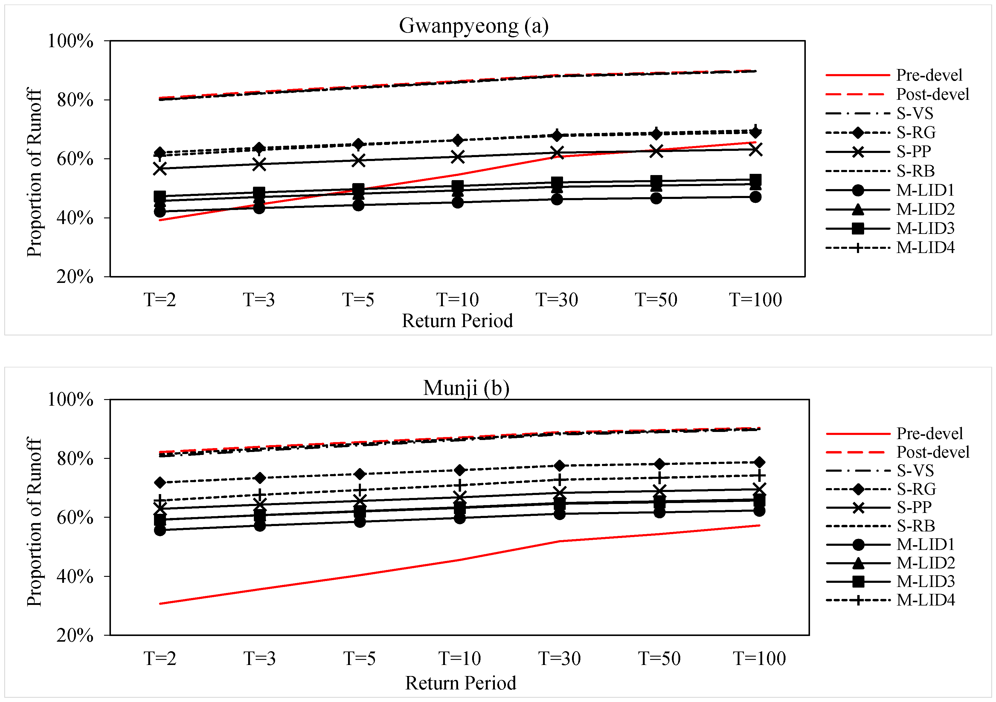
3.3.2. Variation in Surface Runoff

Figure 7 shows the proportional distribution of surface runoff under different simulation scenarios in two case study cites.

The figures show that the surface runoff increases with rainfall return period, and there is a sharp increase in runoff from T = 2 years to T = 30 years, after which the variation trend tends to be moderate. In the pre-development scenario, the proportion of runoff in Gwanpyeong rises dramatically from 39.17% (T = 2 years) to 65.59% (T = 100 years), while the runoff in Munji varies from 30.7% (T = 2 years) to 57.29% (T = 100 years). It means that the discharge capacity before development in Munji is also better than that of Gwanpyeong. Meanwhile, in the post-development scenario, the percentage of surface runoff in Gwanpyeong rise up to 80.64% (T = 2 years) and 89.94% (T = 100 years), and the proportion in Munji increase to 82.2% (T = 2 years) and 90.37% (T = 100 years). It indicates that the runoff rapidly grows with the development of urbanization.

The figures illustrate the drainage capability is enhanced by LIDs to some extent, while the adjusting ability of each LID is different each other. M-LID1 ranks first, followed by M-LID2 and M-LID3. Although the effect of S-PP is much lower than that of M-LID3, it is slightly higher than that of S-RG and M-LID4. S-RB and S-VS occupy the last positions. It is noteworthy that M-LID1 could decrease surface runoff in Gwanpyeong sharply from 80.64% to 42.13% when the return period is two years, nearing the 39.17% before the development of urbanization. Meanwhile, the effect of M-LID2, M-LID3 and S-PP are also superior to those in pre-development scenarios under some certain rainfall conditions. However, in the Munji region, the adjusting ability is not nearly as good as Gwanpyeong. The best effective M-LID1 only could drop the runoff from 90.37% to 62.34%, which is still away from 57.29% in the pre-development scenario (T = 100 years).

In other words, the variation in infiltration and surface runoff before and after development in Figure 6 and Figure 7 illustrate that the hydrological cycle balance in urban regions has been damaged by increasing impervious areas. Figure 6a and Figure 7a show that LIDs in Gwanpyeong could significantly improve the hydrological conditions with the increase in return period. As can be clearly seen in Figure 6b and Figure 7b, although the regulating ability of Munji in hydrological balance is not as dramatic as that of Gwanpyeong, with the increase of rainfall return period, the hydrological distribution of Munji is obviously close to that before development. Therefore, this leads to the conclusion that the hydrological balance regulation ability of LIDs in two regions is enhanced gradually as the increase of rainfall return period.

3.4. Runoff Reduction Analysis

The increasing impermeable area disrupts the hydrological cycle dynamic balance in urban areas; consequently, the risk of waterlogging might increase in urban regions. The variations in the maximum flow and total runoff volume in each LID design scenarios based on the post-development situation were calculated to estimate the risk of waterlogging in urban regions. The runoff reduction performance of LIDs was calculated by the following equation:

$$R=\frac{Q_0-Q_{LID}}{Q_0}\times 100\%$$

(8)

where R is the total variation rate (%), $Q_0$ is the simulated results without LID installation (mm) and $Q_{LID}$ is the simulated results with LID installation (mm).

3.4.1. Peak Flow Reduction

Figure 8 describes the variation trend of the maximum flow after LID implementation in two case sites under different design rainfall return periods. The graphic symbols that combine with the lines signify each LID, which is shown in the explanatory legend in detail.

The figures show that all LIDs, excluding S-RB and S-VS, have an effect on reducing peak flow, and the effect varies with the rainfall return period. In the Gwanpyeong region, there is a dramatic drop in the peak flow reduction rate with the increase of return period. Firstly, all LIDs have a slight fluctuation from T = 2 years to T = 5 years. Then, the variation rates of all LIDs decrease rapidly from T = 5 years to T = 100 years, while the variation of S-RG flatten out from T = 30 years to T = 100 years. Meanwhile, M-LID1 could decrease the peak flow from 44.1% (T = 2 years) to 27.91% (T = 100 years), which ranks the first position. M-LID2 and M-LID3 are next, varying from 39.52% (T = 2 years) to 19.44% (T = 100 years) and from 39.27% (T = 2 years) to 18.43% (T = 100 years), respectively. A dramatic drop is seen in S-PP, M-LID4 and S-RG, decreasing from 26.66% (T = 2 years) to 6.34% (T = 100 years), from 23.07% (T = 2 years) to 3.30% (T = 100 years) and from 20.12% (T = 2 years) to 7.24% (T = 100 years), respectively. However, in the Munji region, there is a slight decrease in peak flow reduction rate with the increase of return period. First, M-LID1, M-LID3 and M-LID4 moderately decrease from 35.02% (T = 2 years) to 33.18% (T = 100 years), from 32.58% (T = 2 years) to 30.87% (T = 100 years) and from 22.0% (T = 2 years) to 20.45% (T = 100 years), respectively. Comparatively, S-RG, S-PP and M-LID2 decrease slightly from 13.51% (T = 2 years) to 12.38% (T = 10 years), from 23.22% (T = 2 years) to 21.86% (T = 10 years) and from 26.15% (T = 2 years) to 25.0% (T = 10 years), respectively. Then, they increase slightly from T = 10 years to T = 100 years, and reach their highest point at 14.79%, 26.44% and 30.97%, respectively, when the return period is 100 years, which may be related to the regional characteristics.

3.4.2. Total Volume Reduction

Figure 9 illustrates the effect of the runoff reduction under different designed LIDs from the perspective of total runoff volume.

The figures show that, excluding S-RB and S-VS, all LIDs have a noteworthy impact on reducing the total runoff volume. In the Gwanpyeong region, there is a moderate drop in the total rainfall volume rate of all LIDs from T = 2 years to T = 100 years. M-LID1, varying from 48.84% (T = 2 years) to 41.67% (T = 100 years), ranks the first place. M-LID2 and M-LID3 occupied the second place, which are changing from 44.3% (T = 2 years) to 36.32% (T = 100 years) and from 42.18% (T = 2 years) to 34.17% (T = 100 years), respectively. Then, S-PP, changing from 30.25% (T = 2 years) to 21.66% (T = 100 years), is slightly higher than that of S-RG and M-LID4, varying from 23.36% (T = 2 years) to 18.09% (T = 100 years) and from 24.68% (T = 2 years) to 14.65% (T = 100 years), correspondingly. However, in the Munji region, all LIDs are relatively stable in different rainfall return periods. M-LID1 varies from 32.24% (T = 2 years) to 29.91% (T = 100 years), which is the best one among all LIDs. M-LID2 and M-LID3, having the same percentages, changed from 27.93% (T = 2 years) to 26.84% (T = 100 years). The change in S-PP from 23.48% (T = 2 years) to 22.19% (T = 100 years) is lower than that of M-LID2 and M-LID3, while it is much higher than that of M-LID4 that fluctuates from 19.98% (T = 2 years) to 16.52% (T = 100 years). M-LID4 is slightly higher than that of S-RG, which alters from 12.54% (T = 2 years) to 13.22% (T = 100 years).

To sum up, Figure 8 and Figure 9 show LIDs could lessen the risk of urban flood to a certain extent, and the regulating ability in the Gwanpyeong region is better than that of Munji. Figure 8a and Figure 9a show that the runoff reduction effect of Gwanpyeong is declined obviously with the return period, while that of Munji possess a stable trend in Figure 8b and Figure 9b. The abnormal trends at Munji is different from the results of previous research studies [13,16]. Considering the results of sensitivity analysis, the impact of the manning roughness coefficient of the conduits are different in two regions. That is, the roughness of the conduits might be the reason for the abnormal results in Munji. To further improve the efficiency of the LIDs under varying rainfall patterns, additional pipe network analysis might be beneficial, which could be a direction for future studies.

4. Conclusions

This study used SWMM to evaluate the hydrological effectiveness in terms of the hydrological balance restoration and runoff reduction in two case study urban regions. The simulation results are summarized as follows.

The hydrological condition has been changing with uncontrollable urbanization, while it is worth noting that LIDs could significantly adjust the dynamic imbalance of the hydrological cycle and even improve the deteriorated conditions to those of the natural condition (before urbanization). They can not only decrease total runoff volume by the use of pervious layer in impermeable areas but also extend the time of concentration, which provides more time for a river in an urban area to drain away the rainwater. Nevertheless, the regulatory effects of LIDs vary with rainfall characteristics. It was concluded that the effect of LIDs in runoff reduction is proved to be more effective during lower storm events, while, with the increase of rainfall, the effect is gradually weakened. Thus, it is necessary to combine the LID designs with the conventional flood control measures to mitigate the risk of urban flooding. This is consistent with the results of previous studies [13,16], but what is different is that the ability to regulate the overall hydrological balance of LIDs is evaluated in this study, and the ability is highlighted with the increase of rainfall return period. Therefore, the main function of LIDs should be oriented toward the restoration of hydrological balance rather than flood mitigation, especially when the rainfall return period is bigger. What should be highlighted here is all rainfall–runoff simulations in the target watersheds were conducted using the rainfall data on a 6-min scale. We compared those results with 1-min interval in the previous study process and found only a small difference. That is, although the time interval of temporal rainfall distribution changed, it has no significant influence on the hydrological function results of LIDs under the same total amount of rainfall.

In the area of the efficiency ranking of eight LIDs, M-LID1(RG + PP + RB + VS) has the highest place, which is followed by M-LID2 (50% PP + RB + RG) and M-LID3 (50% PP + RG + VS). Then, S-PP is lower than t M-LID3, while it is slightly higher than M-LID4 (50% PP + RB + VS). Meanwhile, M-LID4 and S-RG play an equally matched role in most cases, while S-RB and S-VS always occupy the last position. It should be noted that the effectiveness of comprehensive LIDs does not mean the direct superposition of the single LIDs, but actually less than the direct sum of single LIDs.

Furthermore, the overall hydrological performance of LIDs in the Gwanpyeong region is better than that of the Munji region. What is noteworthy is that runoff reduction effect in Gwanpyeong is significantly decrease as rainfall amount, while LIDs possess a stable trend in different rainfall return periods in Munji. On the one hand, the implementation area with LIDs in Gwanpyeong is larger than that in Munji. Although the authors of [12] presented that the increase in the LIDs implementation area does not necessarily mean more efficient, it might be a factor affecting the efficiency. On the other hand, the sensitivity of the hydrological elements in Gwanpyeong is higher than that in Munji, and the impact of the manning roughness coefficient of the conduits are different in two regions. That is, the roughness of the conduits might be the reason for the different results. This paper provides insight into the performance of LIDs under different rainfall characteristics, which is vital for future urban planning.

The following limitations should be further addressed. Firstly, runoff reduction and hydrological cycle balance were primarily analyzed in this study, and other benefits of LIDs, such as recharge of groundwater, should be considered in the future study. In addition, this paper focuses on evaluating the main function of LIDs based on rainfall amounts, in which runoff reduction is proved to be more effective during lower storm events, while, in the case of bigger rainfall amounts, the effect of hydrological balance restoration is better. However, this study analyzed only two developed regions in Korea, therefore does not produce general trends. Further studies should expand to various urban regions. Finally, the roughness of the conduits might be the reason for difference in the effect of LIDs in two regions. The flow velocity is greatly affected by the roughness of pipe; if the velocity is too fast, the peak flow will be too large and lead to waterlogging. Otherwise, if the velocity is too slow, the pollutant will be deposited in the pipe network. In the future, additional pipe network analysis, for example the combined Hardy–Cross method with the optimal control, is needed to estimate the appropriate peak flow.

References

1. Newcomer, M.E.; Gurdak, J.J.; Sklar, L.S.; Nanus, L. Urban recharge beneath low impact development and effects of climate variability and change. Water Resour. Res. 2014, 50, 1716–1734. [Google Scholar] [CrossRef]
2. Zhou, Q. A Review of Sustainable Urban Drainage Systems Considering the Climate Change and Urbanization Impacts. Water 2014, 6, 976–992. [Google Scholar] [CrossRef]
3. Liu, Y.; Bralts, V.F.; Engel, B. Evaluating the effectiveness of management practices on hydrology and water quality at watershed scale with a rainfall-runoff model. Sci. Total Environ. 2015, 511, 298–308. [Google Scholar] [CrossRef] [PubMed]
4. Seo, M.; Jaber, F.; Srinivasan, R.; Jeong, J. Evaluating the Impact of Low Impact Development (LID) Practices on Water Quantity and Quality under Different Development Designs Using SWAT. Water 2017, 9, 193. [Google Scholar] [CrossRef]
5. Satterthwaite, D. The implications of population growth and urbanization for climate change. Environ. Urban. 2009, 21, 545–567. [Google Scholar] [CrossRef] [Green Version]
6. Ahiablame, L.M.; Engel, B.A.; Chaubey, I. Effectiveness of low impact development practices in two urbanized watersheds: Retrofitting with rain barrel/cistern and porous pavement. J. Environ. Manag. 2013, 119, 151–161. [Google Scholar] [CrossRef]
7. Fayetteville, A. LID Low Impact Development: A design Manual for Urban Areas; University of Arkansas Community Design Center: Fayetteville, AR, USA, 2011. [Google Scholar]
8. Li, C.; Liu, M.; Hu, Y.; Han, R.; Shi, T.; Qu, X.; Wu, Y. Evaluating the Hydrologic Performance of Low Impact Development Scenarios in a Micro Urban Catchment. Int. J. Environ. Res. Public Health 2018, 15, 273. [Google Scholar] [CrossRef] [Green Version]
9. Lee, D.C. Restoration of Water Cycle by a Rainwater Management System Applied to Low Impact Development (LID). Ecol. Resilient Infrastruct. 2016, 3, 130–133. [Google Scholar] [CrossRef] [Green Version]
10. Martin-Mikle, C.J.; De Beurs, K.M.; Julian, J.P.; Mayer, P. Identifying priority sites for low impact development (LID) in a mixed-use watershed. Landsc. Urban Plan. 2015, 140, 29–41. [Google Scholar] [CrossRef] [Green Version]
11. Goncalves, M.L.R.; Zischg, J.; Rau, S.; Sitzmann, M.; Rauch, W.; Kleidorfer, M. Modeling the Effects of Introducing Low Impact Development in a Tropical City: A Case Study from Joinville, Brazil. Sustainability 2018, 10, 728. [Google Scholar] [CrossRef] [Green Version]
12. Wu, J.; Yang, R.; Song, J. Effectiveness of low impact development for urban inundation risk mitigation under different scenarios: A case study in Shenzhen, China. Nat. Hazards Earth Syst. Sci. 2018, 18, 2525–2536. [Google Scholar] [CrossRef] [Green Version]
13. Luan, Q.; Fu, X.; Song, C.; Wang, H.; Liu, J.; Wang, Y. Runoff Effect Evaluation of LID through SWMM in Typical Mountainous, Low-Lying Urban Areas: A Case Study in China. Water 2017, 9, 439. [Google Scholar] [CrossRef] [Green Version]
14. Gilroy, K.L.; McCuen, R.H. Spatio-temporal effects of low impact development practices. J. Hydrol. 2009, 367, 228–236. [Google Scholar] [CrossRef]
15. Kong, F.; Ban, Y.; Yin, H.; James, P.; Dronova, I. Modeling stormwater management at the city district level in response to changes in land use and low impact development. Environ. Model. Softw. 2017, 95, 132–142. [Google Scholar] [CrossRef]
16. Zhu, Z.; Chen, X. Evaluating the Effects of Low Impact Development Practices on Urban Flooding under Different Rainfall Intensities. Water 2017, 9, 548. [Google Scholar] [CrossRef]
17. Qin, H.; Li, Z.-X.; Fu, G. The effects of low impact development on urban flooding under different rainfall characteristics. J. Environ. Manag. 2013, 129, 577–585. [Google Scholar] [CrossRef] [Green Version]
18. Koo, Y.M.; Seo, D.G. Parameter estimations to improve urban planning area runoff prediction accuracy using Stormwater Management Model (SWMM). J. Korea Water Res. Assoc. 2017, 50, 303–313. [Google Scholar]
19. Chen, C.-F.; Sheng, M.-Y.; Chang, C.-L.; Kang, S.-F.; Lin, J.-Y. Application of the SUSTAIN Model to a Watershed-Scale Case for Water Quality Management. Water 2014, 6, 3575–3589. [Google Scholar] [CrossRef]
20. Fleischmann, C.M. Evaluating Management Strategies for Urban Stormwater Runoff. Ph.D. Thesis, University of Connecticut, Storrs, CT, USA, 2014. [Google Scholar]
21. Rossman, L.A. Storm Water Management Model User’s Manual; US EPA Office of Research and Development: Washington, DC, USA, 2015.
22. Rawls, W.J.; Brakensiek, D.L.; Miller, N. Green-ampt Infiltration Parameters from Soils Data. J. Hydraul. Eng. 1983, 109, 62–70. [Google Scholar] [CrossRef] [Green Version]
23. Hangzhou Municipal Commission of Urban-Rural Development. Construction Guidelines of Sponge City in Hangzhou. 2016. Available online: http://cxjw.hangzhou.gov.cn/art/2016/10/19/art_1228985153_38649182.html (accessed on 19 October 2018). (In Chinese)
24. IPCC (Intergovernmental Panel on Climate Change). Mitigation of Climate Change—Summary for Policymakers and Technical Summary 2014; Climate Change 2014. Available online: https://www.ipcc.ch/report/ar5/wg3/ (accessed on 9 August 2018).
25. Predrag, P.; Slobodan, P.S. Generation of Synthetic Design Storms for the Upper Thames River Basin. Water Resources Research Report 2004. p. 15. Available online: https://ir.lib.uwo.ca/wrrr/15 (accessed on 9 August 2018).
26. Lee, E.H.; Kim, J.H. Development of a flood-damage-based flood forecasting technique. J. Hydrol. 2018, 563, 181–194. [Google Scholar] [CrossRef]
27. Ahn, J.; Cho, W.; Kim, T.; Shin, H.; Heo, J. Flood Frequency Analysis for the Annual Peak Flows Simulated by an Event-Based Rainfall-Runoff Model in an Urban Drainage Basin. Water 2014, 6, 3841–3863. [Google Scholar] [CrossRef] [Green Version]
28. Korea Precipitation Frequency Data Server. Available online: www.k-idf.re.kr (accessed on 11 August 2018).
29. Ministry of Housing and Urban-Rural Development (MOHURD). Sponge City Construction Technical Guidelines—Construction of Low impact Development Stormwater System. 2014. Available online: http://www.mohurd.gov.cn/wjfb/201411/t20141102_219465.html (accessed on 13 October 2018). (In Chinese)
30. Waseem, M.; Mani, N.; Andiego, G.; Usman, M. A review of criteria of fit for hydrological models. Int. Res. J. Eng. Technol. 2017, 4, 1765–1772. [Google Scholar]
Figure 1. Location of the study area in Daejeon, Korea.
Water 12 02231 g001
Figure 2. Conduit distribution of the study area.
Water 12 02231 g002
Figure 3. Design storms for scenario analysis (6 min): (a) the dimensionless cumulative distribution of Huff method (3rd quartile storm); and (b) the temporal rainfall distribution of 60-min duration.
Water 12 02231 g003
Figure 4. Calibration and validation results for the study areas: (ad) the calibration results of SWMM using R1 to R4; (e) the validation results of SWMM using R5.
Water 12 02231 g004
Figure 5. Sensitive analysis of hydrological parameter in SWMM for the study areas: (ac) the sensitive analysis results based on peak flow, infiltration and runoff volume in Munji; and (df) the sensitive analysis results based on peak flow, infiltration and runoff volume in Gwanpyeong.
Water 12 02231 g005
Figure 6. Proportion of infiltration of different scenarios under different rainfall events at study sites: (a) the results of Gwanpyeong; and (b) the results of Munji.
Water 12 02231 g006
Figure 7. Proportion of runoff of different scenarios under different rainfall events at study sites: (a) the results of Gwanpyeong; and (b) the results of Munji.
Water 12 02231 g007
Figure 8. Variation in LIDs for the maximum flow in two case sites under different rainfall return period: (a) the results of Gwanpyeong; and (b) the results of Munji.
Water 12 02231 g008
Figure 9. Variation in LIDs for the total runoff volume in two case sites under different rainfall return periods: (a) the results of Gwanpyeong; and (b) the results of Munji.
Water 12 02231 g009