Article

Source Apportionment Assessment of Marine Sediment Contamination in a Post-Industrial Area (Bagnoli, Naples)

1
Department of Civil and Environmental Engineering, Politecnico di Milano, 20133 Milano, Italy
2
Department of Engineering, University of Campania, 81031 Caserta, Italy
3
CoNISMa Inter-University National Consortium for Marine Sciences, 00196 Roma, Italy
4
Stazione Zoologica Anton Dohrn, 80121 Napoli, Italy
5
Agenzia Nazionale per le Nuove Tecnologie, L’energia e lo Sviluppo Economico Sostenibile, 00196 Roma, Italy
6
Osservatorio Vesuviano, Istituto Nazionale di Geofisica e Vulcanologia, 80124 Naples, Italy
7
CNR IRISS-Istituto di Ricerca su Innovazione e Servizi per lo Sviluppo, 80124 Napoli, Italy
*
Author to whom correspondence should be addressed.
Water 2020, 12(8), 2181; https://doi.org/10.3390/w12082181
Submission received: 18 June 2020 / Revised: 30 July 2020 / Accepted: 31 July 2020 / Published: 3 August 2020

Abstract

:
The area of Bagnoli (Gulf of Naples, central Tyrrhenian Sea) has been heavily exposed to pollution for over a century due to the presence of industrial sites along its coastline. The aim of this study is to analyze contaminant concentrations (i.e., heavy metals and hydrocarbons) in seabed sediments through a statistical multivariate approach. Multivariate methods permit us to describe the pollution dynamics affecting the area and distinguish between anthropogenic and natural pollution sources. Additionally, the association between contamination patterns and the wave climate characteristics of the gulf (i.e., wave period, direction, height, power, and energy) is investigated. The study confirms that the main contamination source in the Bagnoli bay is anthropogenic activities (i.e., former steel plant and sewage discharges) for the majority of investigated pollutants. It also provides evidence, however, for the potential co-existence of multiple anthropogenic and geogenic sources of arsenic and other metals that may be originating also from the water-rock interaction and submarine volcanic emissions in the Phlegraean area.

1. Introduction

The contamination of marine environments represents an increasing global concern because of the potential risks to both human health and along the coast heavily affecting the marine ecosystems. The Mediterranean Sea, due to reduced circulation and the presence of multiple industrial inputs along the coastline, is particularly vulnerable to environmental impacts and risks. Moreover, there is evidence that contamination may persist long after the end of industrial activities [1]. The historical industrial district and metallurgical production at the Bagnoli steel factory (ILVA), active for roughly a century, has exposed the marine sediments of the Gulf of Pozzuoli (GoP) to pollution by heavy metals and polycyclic aromatic hydrocarbons (PAHs). This area became a key site for twentieth-century Italian economic growth through industrial plants that produced steel and cement using iron ore and coal transported from other locations and processed on site. These activities, now recognized as detrimental to the environment and economically impractical, prompted the industrial area to be dismantled starting in the mid-1990’s [2]. The impact of heavy industries was never completely remediated, however, and this negligence results in high concentrations of PAHs and trace metals in marine sediments [3]. Sediment contamination is still evident in the vicinity of the industrial sites but also widespread in neighboring areas due to re-suspension of sediments and to water currents [4,5,6,7]. Furthermore, sewage loss from wastewater treatment plants or accommodation facilities along the western Bagnoli coastline increased the magnitude of the marine environment contamination [8,9]. Bagnoli has served as the subject of numerous scientific studies aimed at verifying the current condition of the water and marine sediments present in the GoP. Recent work has focused on bioaccumulation and biomarkers investigations to better understand the toxic effects and mechanism of action of contaminants [10,11,12]. Recently, an integrated assessment called sediment quality triad (SQT) was used to consider chemical analyses and biological effects as different lines of evidence (LOEs) to describe environmental quality of marine sediments [2,13]. A multidisciplinary approach (the weight of evidence approach, WoE) permits researchers to interpret various environmental conditions compared to a univariate analysis, such as a chemical approach, and circumvent overestimated and costly management decisions [11]. The WoE approach, integrating five lines of evidence (LOEs: sediment chemistry, bioavailability of chemicals, subcellular effects, toxicity at organism level and at the community level) was successfully applied to the Bagnoli case study and revealed a clearly polluted area but less critical levels of pollution when compared to the results of sediment chemistry alone [2].
This study, developed in the framework of the ABBaCo project which started in 2017, is designed to (a) update and improve the characterization of the environmental quality of the Bagnoli industrial site, (b) identify contamination sources, and (c) propose suitable remediation strategies. In the Bagnoli area, the determination of polluting sources is particularly challenging due to the cohabitation between natural processes and anthropic activities, which assesses sources apportionment more difficult. Moreover, some contaminations are nowadays almost ubiquitous (e.g., PAHs contamination is present in urban areas [14], rural areas [15], and coastal areas [5]).
The GoP is an area characterized by intense volcanic activity due to the presence of a large caldera—the Phlegraean fields—which is one of the most densely populated active volcanoes on Earth. It is characterized by a strong record of historical unrest and eruption events that date back to 2.2 ka BP. Since the 1950’s, the Phlegraean fields’ area has undergone four episodes of caldera-wide uplift and seismicity, which have raised the coastal town of Pozzuoli, near the center of unrest by 4.5 m and triggered the repeated evacuation of some 40,000 people. During the last 20 years of subsidence, following the uplift peak reached in 1984, the caldera started a new, low-rate uplift episode accompanied by low-magnitude seismicity and marked geochemical changes in fumaroles [16]. For this reason, some elements, such as arsenic (As), represent a natural enrichment. In some Italian areas, such as the Po plain, it is recognized that arsenic originates from the reductive dissolution of Fe oxides [17]. Therefore, in the present study, the presence of arsenic is assessable as a characteristic natural background level of the study area [6]. This natural presence of heavy metals in the sea sediments of the gulf is attributed to an active system of submarine thermal springs near the Bagnoli coastline that constantly release volcanic gasses [18,19]. PAHs also originate, however, from percolation through the soils or landfills contaminated by industrial activities [7].
For the assessment of the source apportionment in a highly polluted area, the use of statistical tools is well recognized. Some studies report the advantages of using multivariate statistical analysis [20,21,22,23,24,25,26,27] to interpret the contaminant distributions and the pollutants patterns. For the marine environment, some studies use principal component analysis (PCA) [7,15,28,29,30] and bivariate correlation analysis (Pearson coefficient) [31,32], nonparametric multivariate multiple regression analyses [33,34], canonical analysis of principal coordinates [33], multivariate linkage tree analysis [34] and randomized analysis of variance (PERMANOVA) [8,33,34] to investigate the co-occurrence of a suite of pollutants in sediments and to assess the related response on the biological assemblages that inhabit the seabed. Some correlation analyses were carried out between pollutant concentrations and sediment granulometry [31]. Other studies examined the distribution patterns of the meiofauna and the diversity and abundance of microorganisms inhabiting the sediments of GoP in relation to environmental variation and chemical pollution [8,33,34]. Most PAH inputs in the environment are linked to anthropogenic activity (e.g., wastes from industrialized and urbanized areas, off-shore petroleum hydrocarbons production or petroleum transportation) [35]. One of the main issues is the connection between pollutant concentrations and their possible source (natural or anthropic) combined with the influence of wave climate on their concentration patterns. Within this project, the present research aims to apply a robust statistical approach (PCA/FA) to demonstrate its practical application for assessing the main contamination sources, distinguishing among natural or anthropic/industrial contributions, and finding correlation between the contaminant concentrations and wave hydrodynamics in the area. The workflow framework of the study is shown in Figure 1.

2. Materials and Methods

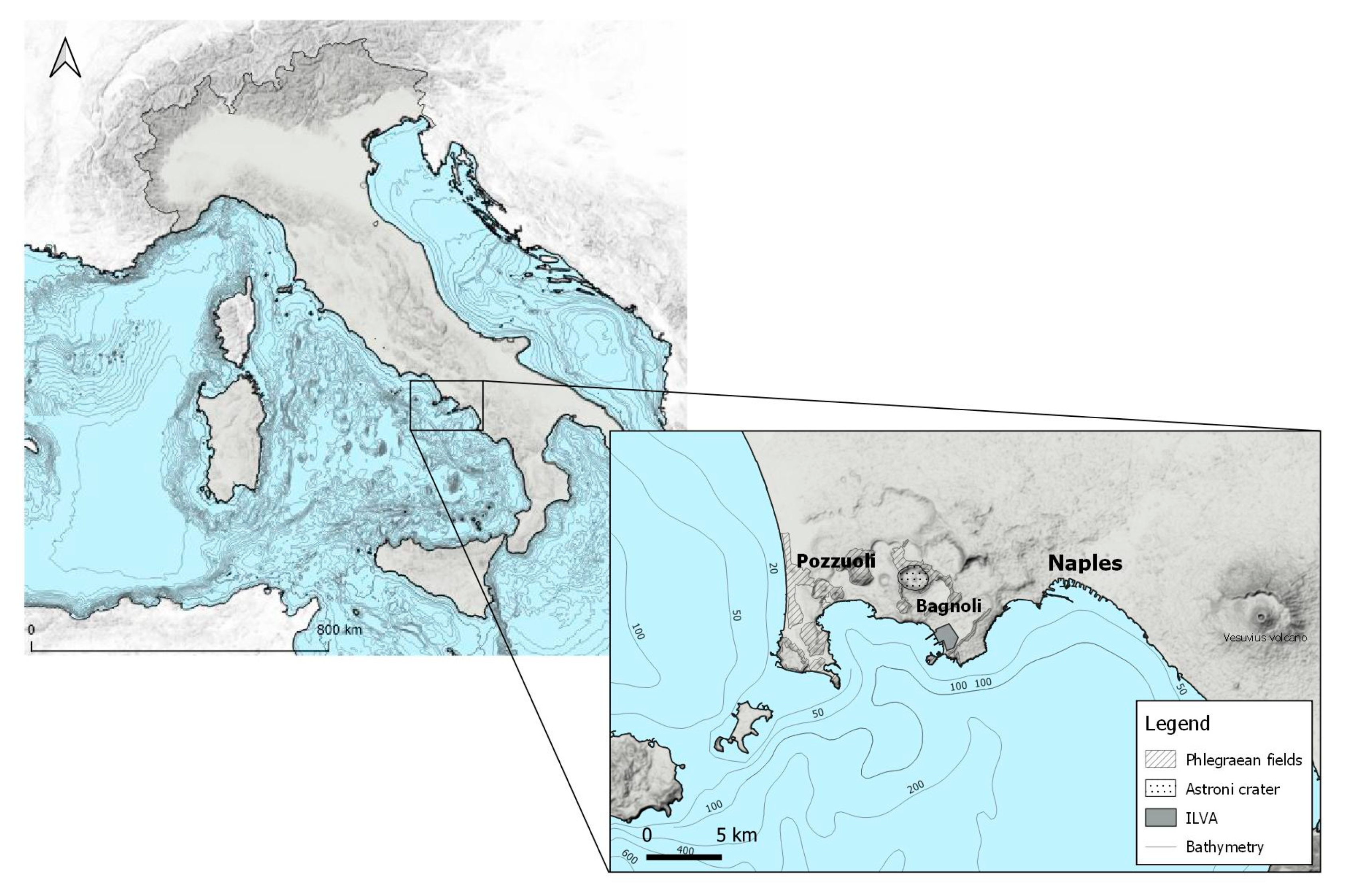
2.1. Study Area and Geological Settings

The study area, Bagnoli, is located within the Bay of Pozzuoli, in the western sector of the urban territory of Naples. Close to the Bagnoli site, the already mentioned Phlegraean fields is a large “super volcano” situated to the west of Naples, Italy. Declared a regional park in 2003, the area of the caldera consists of 24 craters and volcanic edifices, most of them submerged under the bay with very high hydrothermal activity and effusive gaseous manifestations [19] (Figure 2). From a geological point of view, this large caldera is in a state of quiescence. The Phlegraean fields experienced extreme volcanic activity in the last 39,000 years. The two main events occurred 35,000 years ago (the ‘Campanian ignimbrite eruption’), followed by caldera collapse, and 15,000 years ago (the ‘Neapolitan Yellow Tuff’, NYT eruption). The NYT eruption formed the central and eastern part of the Bagnoli–Fuorigrotta plain, which is constituted by a sequence of pyroclastic and volcanic material that thickens along the Agnano crater. Agnano volcanic products dominates the western part of the plain. The last eruptive event occurred in A.D. 1538 and gave rise to the Mt. Nuovo cone. From then on, only bradyseismic and hydrothermal activity (in the Solfatara and Pisciarelli area) are present in the area. The ground deformation in this area was recognized as caused mainly by the actions of long periods of uplift, eruptive activity, and possible deep magma movements [36,37,38]. According to some studies [39], the Phlegraean fields activity has been predominantly explosive and characterized by an interaction between magma and water. There is evidence of both interaction of the magma with sea water as well as intra-caldera lake water and deep-seated aquifers in some Plinian volcanic events. High concentrations of metals and metalloids, such as As, Mn and Fe are found in groundwater and in the sea sediments near the main tectonic and hydrothermal activity [3,18,31,40,41].
Since the early 1900’s Bagnoli has been affected by the presence of various industries. The most important industrial activity was through ILVA steelworks, formerly Italsider. The ILVA steel plant was located along the Bagnoli coastline and was characterized by two long piers (still present now) which served as a berth for large ships that carried raw materials such as coal, iron ore and limestone to the steelworks. In the early 1960’s, in order to enlarge the plant, the area between the two piers was filled with industrial waste coming from the steelworks. A new coastline was designed, giving more space for the industrial activities, but causing consistent damage to the marine ecosystems. Furthermore, the presence of nine discharge points along the coastline, combining both industrial and civil sewage, may have contributed to the deterioration of the quality of the environment. Some of these collectors are no longer in use since the steelworks stopped its production in 1990.
The Bagnoli Bay is also characterized by the presence of some submarine thermal springs, mainly located close to the former industrial area. Some offshore thermal springs are also present in the GoP.

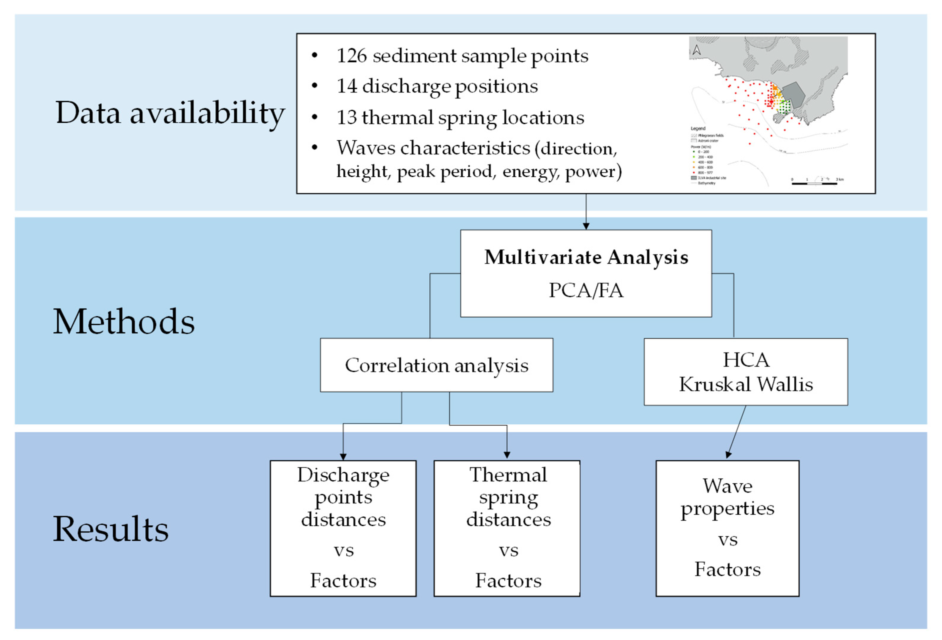
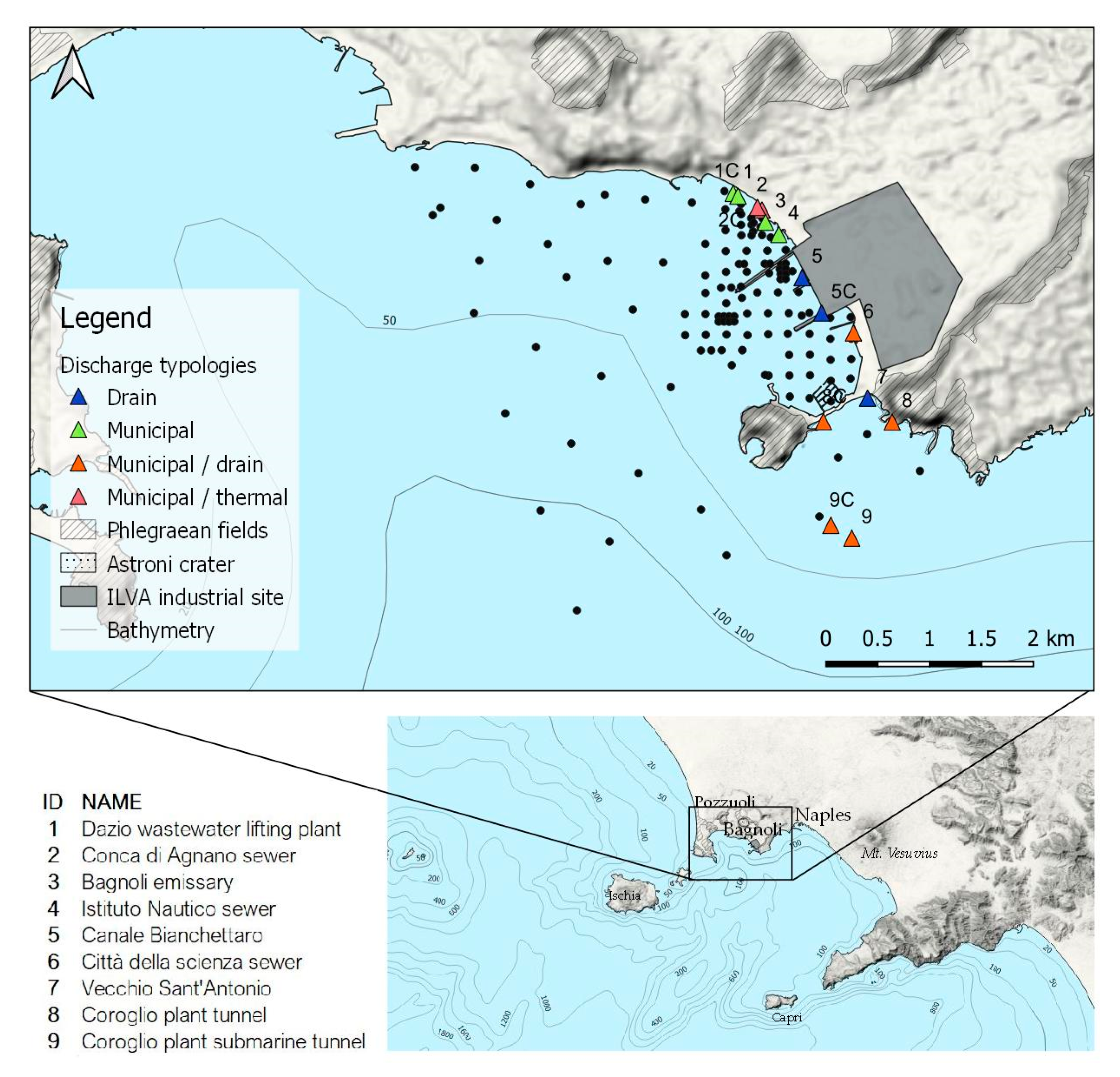
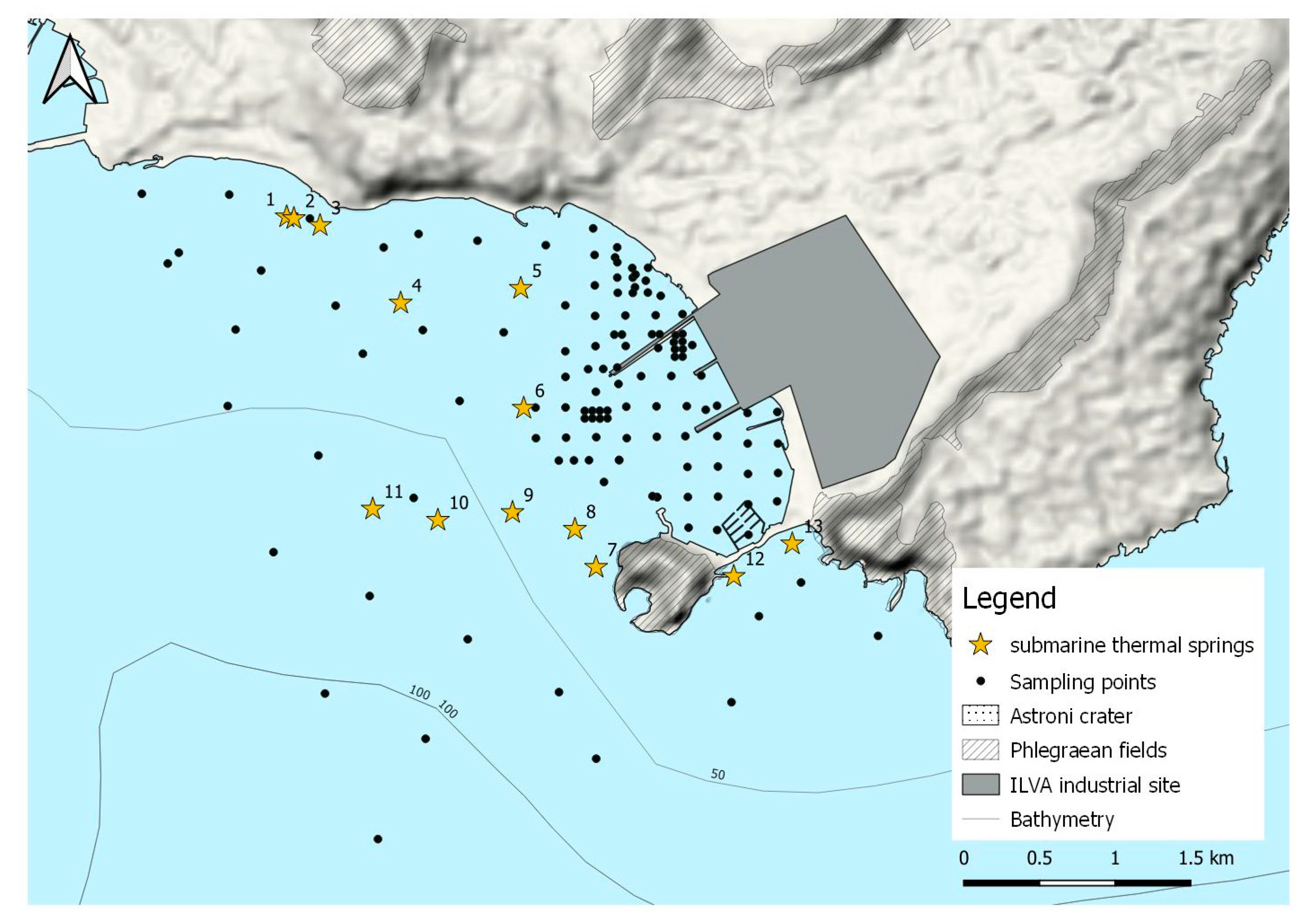
2.2. Data Availability: Sampling, Sewage Discharge, and Wave Information

In this study, a total of 126 sampling points were considered as shown in Figure 3 (black dot points). These samples were part of an explorative campaign carried out in 2017 in the GoP by the Stazione Zoologica Anton Dohrn [42,43]. On the sea bottom, 94 sediment samples were collected using drilling (0-50 cm) and 32 sediment samples were collected by bucket (surface layer). In each point, the concentrations of heavy metals and PAHs were measured. A total of 11 heavy metals (i.e., Al, As, Cd, Cr, Cu, Fe, Hg, Ni, Pb, V, and Zn) and 18 PAHs (i.e., naphthalene, anthracene, phenanthrene, acenaphthylene, acenaphthene, fluorene, fluoranthene, pyrene, benzo(a)anthracene, chrysene, benzo(b)fluoranthene, benzo(a)pyrene, benzo(k)fluoranthene, indeno(1,2,3-cd)pyrene, benzo(ghi)perylene, dibenz(ah)anthracene, benz(j)fluoranthene, benz(e)pyrene) indicated by Environmental Protection Agency (EPA) as important toxicological contaminants were considered. All the samples and the analytical determination derive from the series of studies conducted under the framework of the ABBaCo project [4,33]. Contaminants general statistics are reported in Table 1.
A total of 14 sewage discharge points were mapped and selected in the study area (from 1 to 9C, in Figure 3). Some of these discharge points were supposed to be inactive (e.g., Points 4, 7 and 8). However, it is well recognized that due to poor maintenance and some illegal discharges in sewage disposal these points, especially when heavy rains occur, release water carrying waste and sewage to the coastline. For this reason, all the discharge points shown in the figure have been considered as active. It should also be noted that the discharge points labeled as “C” in Figure 3 are control points chosen as the nearest to discharge point (i.e., 9C is the control point of discharge point 9).
Representing natural contaminant sources spread along the Bagnoli bay seabed, 13 thermal springs were identified [18] (Figure 4).
In addition to the presence of sewage discharges and thermal springs, concentration patterns can be influenced by marine dynamics that remobilize sediments and accumulate them in places where there are steady-state conditions. In order to include the analysis, the main effects of the wave-induced hydrodynamics inside the GoP area in the analysis, we incorporated wave properties generated by a numerical model of the gulf.

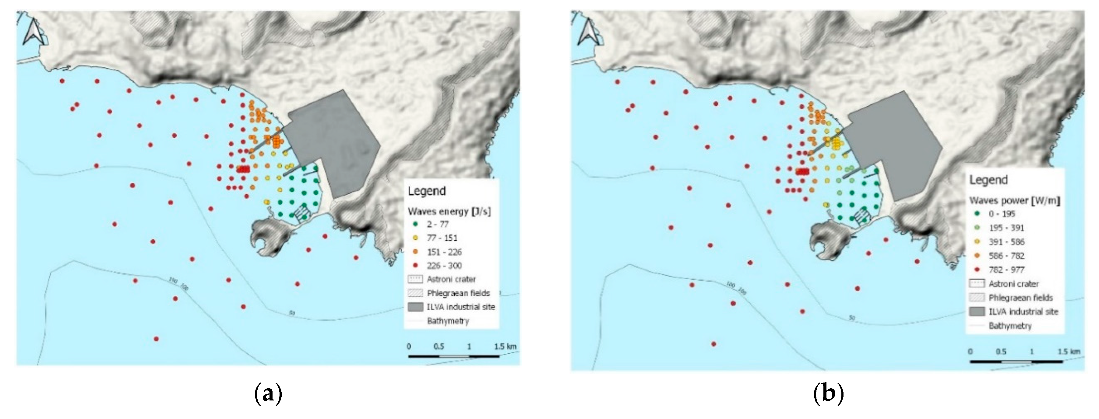
2.3. Numerical Wave Modelling

The wave climate analysis was carried out using the hindcast data from the European Centre for Medium-Range Forecasts (ECMWF). Significant wave height (Hs), mean period (Tm), and mean direction (Θm) for the time period ranging from January 1979 to December 2018 were extracted from the wave model (WAM) of the ERA-interim archive (ERA: ECMWF Atmospheric Reanalysis), available for download online [44]. Both the offshore energetic patterns and the nearshore water conditions have been studied by means of the MIKE 21 SW coastal propagation model [45]. The model has been previously calibrated and validated applying a multi-collocation-based estimation approach as described in [46]. Such studies perform an optimization procedure for:
  • The WAM offshore hindcast data, consisting in an amplification of each value of WAM dataset by means of an “enhancement factor”. The enhancement factor has been obtained by comparison of WAM hindcast dataset at a point located offshore the study area and the time series obtained by transposition of the available data from an offshore wave buoy record. Then, the fictitious WAM time series has been used as input for the numerical model.
  • The nearshores wave propagation model output, applying a two-step calibration strategy by comparison with measurements from acoustic Doppler current profilers and a set of innovative low-cost drifter-derived GPS-based wave buoys [47] located both inside and outside the GoP.
It is worth noting that spreading and dispersion studies and studies of water quality or ecological systems in marine areas are generally carried out by means of coastal hydrodynamic models coupled with sediment transport and particle tracking models. Generally, such modelling is computationally demanding. Therefore, in the perspective to undertake multi-year wave hindcast studies more quickly, a spectral modeling of wave propagation has been used. In order to assess the hypothesis that the bay’s hydrodynamics is a factor of influence on pollution patterns, a single wave scenario able to represent the yearly average condition in the bay in terms of wave energy flux, had to be selected. Such a sea state, here defined as “energy equivalent”, was obtained considering the wave power content of each wave from the whole dataset of 40-year wave records. Operatively, from the 6-h data of Hs, Tm, θm provided by the fictious WAM model, a 6-h wave power and a wave energy dataset were obtained. For a specific sea state, the average wave energy per unit area is proportional to the square of the significant wave height, Hs, according to the known relationship [48]:
E w a v e = 1 16 ρ g H s 2 [ J s ]
where ρ is the sea water density, assumed equal to 1025 kg/ m 3 , g is the gravity acceleration (equal to 9.81 m/s2). For a given spectrum, the significant wave height computation is based on zero-order moment of the spectral function and readily estimated as follows:
H s = H m 0 = 4 m 0
and the wave characteristic/statistic periods can be defined as:
T e = 2 π m 1 m 0
T m = T 01 = 2 π m 0 m 1
where Te, T01 are the energy period and the spectral mean period, respectively, with the spectral moment being defined as:
m n = 0 S ( f ) f n d f
where n = −2, −1, 0, 1, 2, …
The wave power in irregular waves can be computed as:
P = ρ × g 2 × H s 2 × T e 64 × π
Following a conservative approach, according to [49,50], the energy period in the present study has been assumed as 1.14 Tm. Equation (6) can be written in the approximate deep water expression:
P = 0.459 × H s 2 × T e
For each j-th year, an average wave power ( P J ¯ ) has been computed. Considering that the energy period can be computed directly using the approximate formula:
T e = 4.5 × H s
then, an “energetic” yearly significant wave height, He, can be calculated as:
H e , j = P j 0.459 × 4.5 2.5
for j = 1, …, 40, and a correspondent energy period can be estimated as follows:
T e e , j = 4.5 × H e , j
The 40-year average for these parameters gives H e = 0.93   m and T e e = 4.3   s .   Regarding the representative direction, De, a vectoral analysis about the energy flows (carried out comparing records of ADCP installed in the bay and correspondent offshore waves) indicate as the offshore wave direction can be considered 217° N. Finally, the “energy equivalent scenario” with He, Tee and De has been propagated applying the MIKE 21 SW model. The seabed was performed by interpolating at the grid nodes the information provided by the General Bathymetric Chart of the Oceans (GEBCO) database [51]. A gross verification of the 10-m isobath, as representative of the nearshore region in a wave propagation model, has been applied by comparison with a recent bathymetric campaign [19].

2.4. Statistical Analysis: Multivariate Analysis and Bivariate Correlation

All the statistical computations were implemented using the statistical software IBM SPSS Statistics® (version 26.0), while spatial queries, distance calculation and data mapping were managed through the open source environmental software QGIS (version 3.8.3, https://qgis.org/en/site/).
PCA [52] is a powerful technique to investigate patterns of correlations among a set of variables. PCA in fact allows to extract a set of new variables, uncorrelated, called principal components (herein after PCs), each aggregating the variables more strongly correlated with the PC and among themselves. PCA seeks in fact a linear combination of input variables, which extracts the maximum variance of the bivariate correlation matrix. Following this, with a second linear combination, orthogonal from the first one, PCA extracts the maximum variance of the remaining variance, and so on. PCs represent all the linear combinations of the original variables weighted by their contribution in explaining the variance, in a specific orthogonal dimension. PCA was turned into a factor analysis (FA) to reduce the contribution of the less significant parameters within each component, by extracting a new set of vari-factors through rotating the axes defined by the PCA extraction. The Varimax rotation criterion was used to rotate the PCA axes allowing us to maintain the axes, orthogonality. The number of factors to be retained was chosen based on the “eigenvalue higher than 1” criterion (i.e., all the factors that explained less than the variance of one of the original variables were discarded).
To assess the variability within the whole set of contaminants, PCA/FA was performed considering all 11 metals, and all 18 PAHs (Table 1). For each of the N sampling points, PCA enabled to calculate principal component scores aggregating the information of the different parameters’ concentration values. Moreover, in order to assess correlations between the sampled contaminants concentrations and the position of sewage discharges and thermal springs, a distance matrix was created through the QGIS vector toolbox, containing the pairwise distance between each sampling point and each discharge point. The measurements-discharges distance matrix was then associated to the component loadings and a bivariate Pearson’s linear correlation analysis was performed. Finally, in order to assess the possible effects of the waves’ dynamics on the concentration patterns found with PCA, a Kruskal Wallis test was performed to test the significance of hydrodynamics’ effect on the contaminant concentrations, likewise similar studies [53,54,55,56]. Five wave characteristics were considered, such as the direction, the height, the mean peak period, the energy and the resulting power of the wave motion inside the bay. These characteristics were subdivided into classes, identified based on a hierarchical cluster analysis (HCA) [52] and tested as factors on the vari-factors assumed as dependent variable in the Kruskal Wallis test. Therefore, the KW null hypothesis was the equality of the vari-factor medians across wave characteristics classes. The level of significance assumed was P-value lower than 0.05.

3. Results

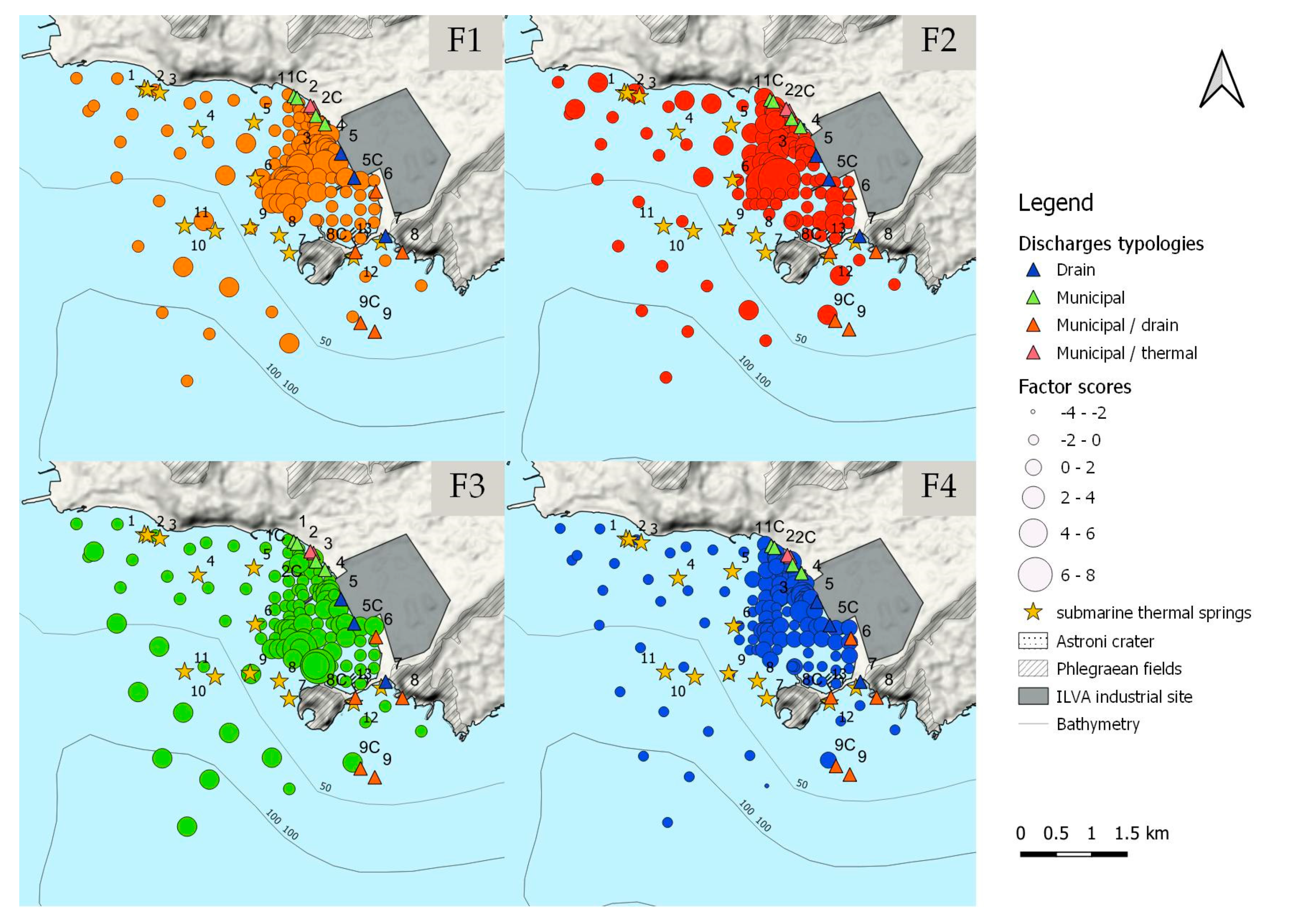
3.1. PCA and PCs Extraction

PCA/FA allowed us to extract four rotated PCs accounting for about 86% of cumulative variance from the original 29 variables. Table 2 shows the matrix of the Factor loadings, which represent the correlation of each variable with each rotated PCs.
Based on factor loadings, the Factors can be interpreted as follows:
  • F1 accounts for 38.3% of the variance and it is loaded mostly by PAHs and by some heavy metals (i.e., Cd, Cu, Fe).
  • F2 accounts for 35.4% of the variance and it is loaded by the remaining PAHs with a lower molecular weight and higher vapor pressure.
  • F3 accounts for 6.8% of the variance and it is loaded by Cr, Ni and V.
  • F4 accounts for 5.5% of the variance and it is loaded by As.
PCA/FA highlights that PAHs concentrations are split into two different pollution components and this is consistent with their mobility characteristics. The molecular weight is in fact considered as an index of the dispersion of a pollutant: the heavier a substance is, in terms of molecular weight, the lower their environmental mobility is (Supplementary Materials: Table S1 shows the PAH molecular weights).

3.2. Factors vs. Sewage Discharges

After the factors identification, a bivariate correlation analysis with the distances from the existent discharges was performed. In Table 3, the Pearson’s linear correlation coefficients are shown. It can be observed that the significant correlations are all negative, outlining that higher is the distance of the sampling point from the discharge point, the lower is the pollutant concentration. It is also worthwhile to observe that the points labeled as C, control points of the specific discharge points, show the same pattern of correlation of actual discharge points.
The results show that the pollutants included in F1 are inversely correlated with the distance from the discharges 5 and 5C (i.e., the discharge and the control point of the former industrial area). No significant correlations were instead found between the pollutants loaded on F2 and the distances from the discharges, while F3, including Cr, Ni and V, correlates inversely with 8C, 9, 9C discharge points. These discharges are located on the southern side of the Nisida isthmus and are the discharges of the Coroglio Plant 8 and 9 (Figure 3). Finally, F4 showed significant correlations with distances from all discharges except 9 (and 9C). Being F4 loaded only by As, it may be speculated that As concentrations did not depend on specific discharge points, but it may rather derive from the whole coastal area and it is distributed along the whole gulf. The geology of the land surrounding the gulf (i.e., pyroclastic rocks) had in fact characteristics that were consistent with a geogenic origin of the As. Moreover, this analysis suggested that the presence of As in sediments is not necessarily due to the industrial spillage, but it may have a possible natural origin related to the geology of the area.
Based on these results, F2 was the only pollution component, which was not found correlated with any discharge point. This can be a consequence of the higher mobility of these compounds and their tendency to disperse.

3.3. Factors vs. Thermal Springs

As mentioned before, F4 (representative of As contamination pattern) resulted to be inversely correlated to the majority of the discharge points located along the Bagnoli coastline, suggesting that the As contamination in the gulf might not be due to a single source, but it may be caused by a presence of multiple sources (i.e., discharged into the gulf through groundwater). In addition, As might be released through submarine thermal springs that were clustered on the Pozzuoli Bay seabed. In order to investigate this possibility, another correlation analysis was performed. Being As loaded only on F4, the other three components were excluded from this analysis (Table 4).
Some positive correlations between As and the distance from Thermal Springs 10 and 11 were found, whereas inverse correlations were found with T5, T6, T12 and T13. Such an ambiguous pattern might be attributed to the fact that only some of those hydrothermal springs were fully active as was shown by recent studies [16,18,19]. As some of those springs are located in the open sea, the positive correlations might be the effect of the bathymetry of the bay [19], where the seabed sinks rapidly from the coastal area, determining the coastal accumulation of the sediments enriched with As.
It is also worth noting that these springs were in the proximity of discharge points (e.g., Thermal Springs 5 and 6 which are close to the “Conca d’Agnano”, Discharge 2, or Thermal springs 12 and 13, which are close to Discharges 8 and 9, shown in Figure 3). All these drains are likely to be affected by groundwater and thermal water infiltrations which may possibly contain As [57].

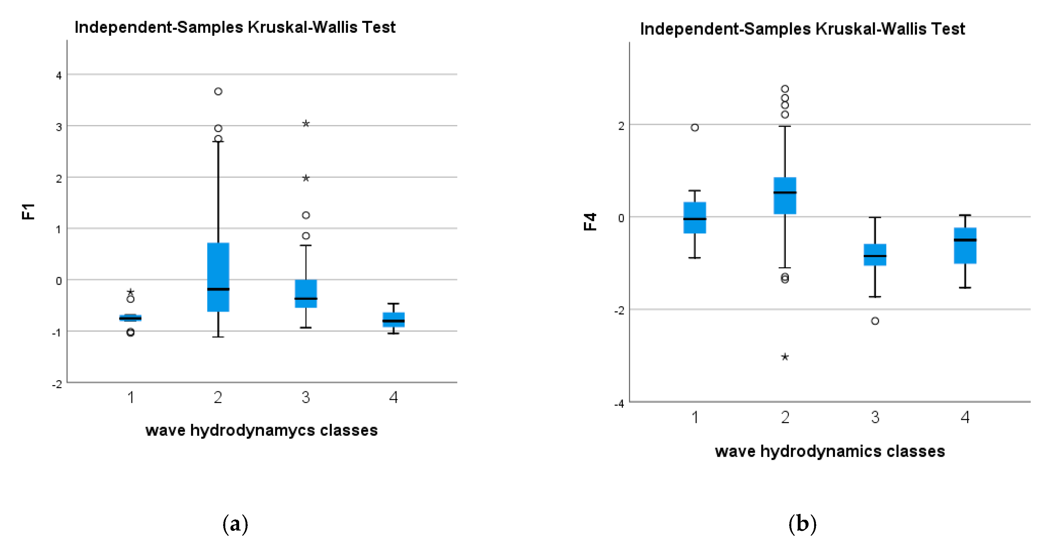
3.4. Pollution Patterns and Wave Hydrodynamics

In order to assess whether the wave hydrodynamics have an influence on pollutant concentrations in sediments, the wave characteristics estimated at each sampling point were interpolated and pollutant vari-factors were tested against five classes of wave characteristic (i.e., wave height, peak period and mean direction) through the Kruskal Wallis test. Figure 5 shows the bathymetry implemented in the wave numerical model, the significant wave height and the energy period as results of the wave propagation of the 40-year averaged energy equivalent scenario.
Besides wave height, peak period and mean direction, the energy content and the energy flux were also calculated. Figure 6 showed the distribution of the wave energy and wave power at each sampling point.
HCA results suggested to subdivide the wave hydrodynamics profiles of the Gulf into four classes of increasing hydrodynamics/energy (see Table 5). These classes have been tested as fixed factors in the Kruskal Wallis test design.
The different pollution components (i.e., F1, F2, F3 and F4) showed different results:
  • F1, loaded by the heavier PAH compounds and by some heavy metals and F4 loaded by arsenic, were both found significantly influenced by wave hydrodynamics (test results were respectively H: 12.9; df: 3, P < 0.01; and H: 51; df: 3, P < 0.01).
  • F2, loaded by the lighter PAHs, and F3, loaded by chromium, nickel and vanadium were not found influenced by the wave hydrodynamics (P > 0.05).
Moreover, pairwise comparisons where significance values have been adjusted by the Bonferroni correction for multiple tests allowed to assess that the F1 pollution component had the highest concentration values associated with classes of intermediate hydrodynamics (P < 0.05, see Figure 7a.) whereas F4 (and therefore arsenic) was found mostly associated with a low hydrodynamics (P < 0.05, see Figure 7b.).
Therefore, the PAHs’ F1 component appears to be affected by the wave-induced currents, being the concentration pattern of these pollutants in sediments dependent also on the shallow water hydrodynamic parameters in the bay. On the other hand, the wave hydrodynamics was not found to influence the PAHs’ F2 component whose higher mobility had probably contributed to homogenize their contamination level in the bay. Likewise, F3 pollutants (i.e., chromium, nickel and vanadium) do not any the wave-induced pattern in the bay. Arsenic (F4) instead was found strongly associated to the areas closest to the coast and characterized by a low wave hydrodynamics.

4. Discussion

This study confirms that a multivariate statistical analysis (PCA/FA) approach can be extremely effective in assessing the apportionment of contaminant sources, even in a site with a complex geological characteristic and a long historical industrial development. With respect to the previous studies (e.g., [3,4,6,7,18]) which used similar methods to investigate the sediments or biota ([31,33,34]), this study considers a larger portion of the Gulf of Bagnoli, and it investigates the relationship of metals/PAHs with both the hydrodynamics of the Gulf and potential discharges/sources. Additionally, while studies in literature considered mostly the sum of total PAHs, in this study 18 PAH compounds are considered individually as their contamination pattern in the gulf. This aspect of the analysis allows us to determine that PAHs of higher molecular weight follow the pattern of metals such as Cd, Cu, Hg, Pb, Zn and Fe and are mainly located near the former discharges of the ILVA steelwork plant. PAHs of lower molecular weight are more dispersed in the gulf. Moreover, while heavier compounds seemed to be influenced by the wave climate of the bay, lighter compounds were apparently much less influenced by it.
Heavy metals such as chromium, nickel and vanadium were found more concentrated near the Nisida northwestern coast and in offshore waters (Figure 8) and did not appear to be strongly influenced by the wave hydrodynamics of the outer gulf. These findings were coherent with the findings of other studies ([4,6,58,59]) even though the measurements in this study derived mostly from drilling and did not include sediment cores.
Armiento et al. [4] within the same ABBaCo framework had analyzed both drilling (i.e., top layer sediments or TL) and sediment cores and found that that TL samples were characterized by a lower contamination than sediment cores. It is important to note that the correlation patterns found in TL samples reflected what was found in studies that analyzed historical contamination patterns through sediment cores.
The association of Cd, Cu, Hg, Pb, Zn and PAHs was described by Romano et al. through the analysis of sediment cores in a study [6] that determined the historical contamination pattern from industrial activity. The same study found that As, Cr, Ni and V were associated with deeper levels (209–299 cm) of the cores having with the highest percentages of clay fraction, suggesting a prevalent natural contribution for these elements. The only contaminant that is almost completely uncorrelated with the other pollutants is arsenic. This metalloid is significantly present in the bay showing a gradient from offshore to the inshore zones. Arsenic variability was found significantly correlated with both the distance from discharge sites located along the coastline and with some thermal springs present on the seabed. This pattern suggests that it is impossible to attribute the origin to a single source, even when the anthropogenic or the geogenic origin is slightly dominant.
Finally, our study confirms that arsenic is not correlated with other elements and highlights that the spatial pattern of its contamination might be dependent on both a land-driven origin (e.g., As-enriched groundwater, see [58]) and the presence of subaerial/submarine geothermal springs [59]).
The correlation of arsenic with the sewage discharge sites suggests a potential effect due to multiple anthropic activities: the former ILVA steelworks used arsenic in their production cycle but glass factories, located along the coastline in the past, may have contributed to the contamination due to their use of arsenic in glass production. Furthermore, the correlation with thermal springs might account for a “natural” arsenic source and conditions are not infrequent where discharges are characterized by a mixture of anthropogenic and geogenic sources. One example of this is the Conca d’Agnano discharge point which releases a mix of water from Agnano lake (i.e., thermal) and municipal wastewaters. Sewage discharge might also contain As-enriched groundwaters due to gas-water-rock interactions inside the aquifer [57,60]. The diffusion of arsenic in the bay was found to be influenced by the wave hydrodynamics, suggesting that arsenic dispersion in sediments might be attributed to various sources (anthropic, natural, or “mixed”) and further diffused due to the particular marine dynamics in the Bagnoli Bay.

5. Conclusions

The results of this study contribute to the reconstruction of the contamination history of the Bagnoli coastal zone, determined by the presence and past activity of industrial sites. Due to the high urbanization of the Neapolitan coastal zone it is impossible to find an unpolluted area-characterized by the same natural environmental framework of the impacted industrial site—to use as a control area. In the present study, a PCA/FA assessment was carried out in the Bagnoli Bay in order to demonstrate the utility of the robust statistical tool in a complex environmental/industrial scenario to investigate the concentrations’ variability and their relationship with the locations of sewers, industrial sites, thermal springs, and the wave action inside the GoP. This study confirms the importance of performing statistically robust multidimensional analysis to support the source apportionment assessment of marine sediment contamination. PCA/FA, considering several parameters, allowed better discrimination among the many contamination components affecting the Bagnoli Gulf area and proved to be a very powerful tool in a complex environment with a mixture of effects due to anthropogenic and natural sources. The results of the analyses confirm that the main contamination source is anthropogenic activities (i.e., former steel plant and sewage discharges) but it also suggests the existence of multiple anthropogenic and geogenic sources of arsenic and other metals that might be originating from the volcanic rocks present in the Phlegraean area.
These findings suggest the need to define a “natural background level” (NBL) for the area for arsenic and other heavy metals to distinguish the natural from the anthropogenic component of the contamination. The source apportionment assessment presented here may help define such NBLs, and also facilitate decisions on the contamination control and the remediation management of the area, permitting public authorities to apply knowledge-based management actions.

Supplementary Materials

The following are available online at https://www.mdpi.com/2073-4441/12/8/2181/s1, Table S1: The molecular weights of PAHs, split into to their principal components.

Author Contributions

Conceptualization and methodology: all authors contributed equally. Data interpretation, A.A., R.S., S.G.; resources, D.V., L.M., P.C., G.A.; writing—original draft preparation, S.G. and L.C., A.A.; writing—review and editing, all authors contributed equally. All authors have read and agreed to the published version of the manuscript.

Funding

This research was funded by the Italian Ministry for Education, University and Research (MIUR) through the ABBaCo project, grant number C62F16000170001.

Acknowledgments

We thank “Anton Dohrn” Zoological Station, ISPRA (Institute for the Environmental Protection and Research), CNR (National Research Center), INGV (National Institute of Geophysics and Volcanology) and INVITALIA for providing the information about Bagnoli Bay and about available datasets PAHs and heavy metals concentrations. We thank also Università degli Studi Luigi Vanvitelli for providing the characterization of the Bagnoli Bay wave climate. Further, we gratefully acknowledge Karen Holmberg for having read the paper, giving useful suggestions and correcting the English version. We also thank two anonymous reviewers for useful suggestions, which helped to clarify and improve the paper.

Conflicts of Interest

All authors declare no conflicts of interest.

References

  1. Richir, J.; Salivas-Decaux, M.; Lafabrie, C.; Lopez y Royo, C.; Gobert, S.; Pergent, G.; Pergent-Martini, C. Bioassessment of trace element contamination of Mediterranean coastal waters using the seagrass Posidonia oceanica. J. Environ. Manag. 2015, 151, 486–499. [Google Scholar] [CrossRef] [PubMed]
  2. Morroni, L.; d’Errico, G.; Sacchi, M.; Molisso, F.; Armiento, G.; Chiavarini, S.; Rimauro, J.; Guida, M.; Siciliano, A.; Ceparano, M.; et al. Integrated characterization and risk management of marine sediments: The case study of the industrialized Bagnoli area (Naples, Italy). Mar. Environ. Res. 2020, 160, 104984. [Google Scholar] [CrossRef]
  3. Romano, E.; Ausili, A.; Zharova, N.; Celia Magno, M.; Pavoni, B.; Gabellini, M. Marine sediment contamination of an industrial site at Port of Bagnoli, Gulf of Naples, Southern Italy. Mar. Pollut. Bull. 2004, 49, 487–495. [Google Scholar] [CrossRef] [PubMed]
  4. Armiento, G.; Caprioli, R.; Cerbone, A.; Chiavarini, S.; Crovato, C.; De Cassan, M.; De Rosa, L.; Montereali, M.R.; Nardi, E.; Nardi, L.; et al. Current status of coastal sediments contamination in the former industrial area of Bagnoli-Coroglio (Naples, Italy). Chem. Ecol. 2020, 36(6), 579–597. [Google Scholar] [CrossRef]
  5. Arienzo, M.; Donadio, C.; Mangoni, O.; Bolinesi, F.; Stanislao, C.; Trifuoggi, M.; Toscanesi, M.; Di Natale, G.; Ferrara, L. Characterization and source apportionment of polycyclic aromatic hydrocarbons (pahs) in the sediments of gulf of Pozzuoli (Campania, Italy). Mar. Pollut. Bull. 2017, 124, 480–487. [Google Scholar] [CrossRef]
  6. Romano, E.; Bergamin, L.; Celia Magno, M.; Pierfranceschi, G.; Ausili, A. Temporal changes of metal and trace element contamination in marine sediments due to a steel plant: The case study of Bagnoli (Naples, Italy). Appl. Geochem. 2018, 88, 85–94. [Google Scholar] [CrossRef]
  7. Trifuoggi, M.; Donadio, C.; Mangoni, O.; Ferrara, L.; Bolinesi, F.; Nastro, R.A.; Stanislao, C.; Toscanesi, M.; Di Natale, G.; Arienzo, M. Distribution and enrichment of trace metals in surface marine sediments in the Gulf of Pozzuoli and off the coast of the brownfield metallurgical site of Ilva of Bagnoli (Campania, Italy). Mar. Pollut. Bull. 2017, 124, 502–511. [Google Scholar] [CrossRef]
  8. Bertocci, I.; Dell’Anno, A.; Musco, L.; Gambi, C.; Saggiomo, V.; Cannavacciuolo, M.; Lo Martire, M.; Passarelli, A.; Zazo, G.; Danovaro, R. Multiple human pressures in coastal habitats: Variation of meiofaunal assemblages associated with sewage discharge in a post-industrial area. Sci. Total Environ. 2019, 655, 1218–1231. [Google Scholar] [CrossRef]
  9. Jenkins, S.H. Mediterranean Coastal Pollution: Proceedings of a Conference Held in Palma; Pergamon Press: New York, NY, USA, 1980. [Google Scholar]
  10. Regoli, F.; Giuliani, M.E. Oxidative pathways of chemical toxicity and oxidative stress biomarkers in marine organisms. Mar. Environ. Res. 2014, 93, 106–117. [Google Scholar] [CrossRef]
  11. Regoli, F.; d’Errico, G.; Nardi, A.; Mezzelani, M.; Fattorini, D.; Benedetti, M.; Di Carlo, M.; Pellegrini, D.; Gorbi, S. Application of a weight of evidence approach for monitoring complex environmental scenarios: The case-study of off-shore platforms. Front. Mar. Sci. 2019, 6, 377. [Google Scholar] [CrossRef]
  12. Menghan, W.; Stefano, A.; Annamaria, L.; Claudia, C.; Antonio, C.; Wanjun, L.; Marco, S.; Angela, D.; Benedetto, D.V. Compositional analysis and pollution impact assessment: A case study in the Gulfs of Naples and Salerno. Estuar. Coast. Shelf Sci. 2015, 160, 22–32. [Google Scholar] [CrossRef]
  13. Chapman, P.M. Determining when contamination is pollution—Weight of evidence determinations for sediments and effluents. Environ. Int. 2007, 33, 492–501. [Google Scholar] [CrossRef] [PubMed]
  14. Colombo, L.; Alberti, L.; Mazzon, P.; Formentin, G. Transient Flow and Transport Modelling of an Historical CHC Source in North-West Milano. Water 2019, 11, 1745. [Google Scholar] [CrossRef] [Green Version]
  15. Stevenazzi, S.; Masetti, M.; Beretta, G. Pietro Groundwater vulnerability assessment: From overlay methods to statistical methods in the Lombardy Plain area. Acque Sotter.-Ital. J. Groundw. 2017, 6, 1–11. [Google Scholar]
  16. Troise, C.; De Natale, G.; Schiavone, R.; Somma, R.; Moretti, R. The Campi Flegrei caldera unrest: Discriminating magma intrusions from hydrothermal effects and implications for possible evolution. Earth-Sci. Rev. 2019, 188, 108–122. [Google Scholar] [CrossRef]
  17. Rotiroti, M.; Sacchi, E.; Fumagalli, L.; Bonomi, T. Origin of Arsenic in Groundwater from the Multilayer Aquifer in Cremona (Northern Italy). Environ. Sci. Technol. 2014, 48, 5395–5403. [Google Scholar] [CrossRef]
  18. Albanese, S.; De Vivo, B.; Lima, A.; Cicchella, D.; Civitillo, D.; Cosenza, A. Geochemical baselines and risk assessment of the Bagnoli brownfield site coastal sea sediments (Naples, Italy). J. Geochem. Explor. 2010, 105, 19–33. [Google Scholar] [CrossRef]
  19. Somma, R.; Iuliano, S.; Matano, F.; Molisso, F.; Passaro, S.; Sacchi, M.; Troise, C.; De Natale, G. High-resolution morpho-bathymetry of Pozzuoli Bay, southern Italy. J. Maps 2016, 12, 222–230. [Google Scholar] [CrossRef]
  20. Idowu, O.; Carbery, M.; O’Connor, W.; Thavamani, P. Speciation and source apportionment of polycyclic aromatic compounds (PACs) in sediments of the largest salt water lake of Australia. Chemosphere 2020, 246, 125779. [Google Scholar] [CrossRef]
  21. Yuanan, H.; He, K.; Sun, Z.; Chen, G.; Cheng, H. Quantitative source apportionment of heavy metal(loid)s in the agricultural soils of an industrializing region and associated model uncertainty. J. Hazard. Mater. 2020, 391, 122244. [Google Scholar] [CrossRef]
  22. Henriksson, S.; Hagberg, J.; Bäckström, M.; Persson, I.; Lindström, G. Assessment of PCDD/Fs levels in soil at a contaminated sawmill site in Sweden—A GIS and PCA approach to interpret the contamination pattern and distribution. Environ. Pollut. 2013, 180, 19–26. [Google Scholar] [CrossRef] [PubMed]
  23. Meng, L.; Zuo, R.; Wang, J.-S.; Yang, J.; Teng, Y.-G.; Shi, R.-T.; Zhai, Y.-Z. Apportionment and evolution of pollution sources in a typical riverside groundwater resource area using PCA-APCS-MLR model. J. Contam. Hydrol. 2018, 218, 70–83. [Google Scholar] [CrossRef] [PubMed]
  24. Rahman, M.S.; Hossain, M.B.; Babu, S.M.O.F.; Rahman, M.; Ahmed, A.S.S.; Jolly, Y.N.; Choudhury, T.R.; Begum, B.A.; Kabir, J.; Akter, S. Source of metal contamination in sediment, their ecological risk, and phytoremediation ability of the studied mangrove plants in ship breaking area, Bangladesh. Mar. Pollut. Bull. 2019, 141, 137–146. [Google Scholar] [CrossRef] [PubMed]
  25. Azzellino, A.; Colombo, L.; Lombi, S.; Marchesi, V.; Piana, A.; Merri, A.; Alberti, L. Groundwater diffuse pollution in functional urban areas: The need to define anthropogenic diffuse pollution background levels. Sci. Total Environ. 2019, 656, 1207–1222. [Google Scholar] [CrossRef]
  26. Alamdar, R.; Kumar, V.; Moghtaderi, T.; Naghibi, S.J. Groundwater quality evaluation of Shiraz City, Iran using multivariate and geostatistical techniques. SN Appl. Sci. 2019, 1, 1367. [Google Scholar] [CrossRef] [Green Version]
  27. Sheikhy Narany, T.; Ramli, M.F.; Aris, A.Z.; Sulaiman, W.N.A.; Fakharian, K. Spatiotemporal variation of groundwater quality using integrated multivariate statistical and geostatistical approaches in Amol-Babol Plain, Iran. Environ. Monit. Assess. 2014, 186, 5797–5815. [Google Scholar] [CrossRef]
  28. Lattuada, M.; Albrecht, C.; Wilke, T. Differential impact of anthropogenic pressures on Caspian Sea ecoregions. Mar. Pollut. Bull. 2019, 142, 274–281. [Google Scholar] [CrossRef] [Green Version]
  29. Bajt, O.; Ramšak, A.; Milun, V.; Andral, B.; Romanelli, G.; Scarpato, A.; Mitrić, M.; Kupusović, T.; Kljajić, Z.; Angelidis, M.; et al. Assessing chemical contamination in the coastal waters of the Adriatic Sea using active mussel biomonitoring with Mytilus galloprovincialis. Mar. Pollut. Bull. 2019, 141, 283–298. [Google Scholar] [CrossRef]
  30. Stefania, G.A.; Rotiroti, M.; Buerge, I.J.; Zanotti, C.; Nava, V.; Leoni, B.; Fumagalli, L.; Bonomi, T. Identification of groundwater pollution sources in a landfill site using artificial sweeteners, multivariate analysis and transport modeling. Waste Manag. 2019, 95, 116–128. [Google Scholar] [CrossRef]
  31. Romano, E.; Bergamin, L.; Ausili, A.; Pierfranceschi, G.; Maggi, C.; Sesta, G.; Gabellini, M. The impact of the Bagnoli industrial site (Naples, Italy) on sea-bottom environment. Chemical and textural features of sediments and the related response of benthic foraminifera. Mar. Pollut. Bull. 2009, 59, 245–256. [Google Scholar] [CrossRef]
  32. Sinaei, M.; Zare, R. Polycyclic aromatic hydrocarbons (PAHs) and some biomarkers in the green sea turtles (Chelonia mydas). Mar. Pollut. Bull. 2019, 146, 336–342. [Google Scholar] [CrossRef] [PubMed]
  33. Gambi, C.; Dell’Anno, A.; Corinaldesi, C.; Lo Martire, M.; Musco, L.; Da Ros, Z.; Armiento, G.; Danovaro, R. Impact of historical contamination on meiofaunal assemblages: The case study of the Bagnoli-Coroglio Bay (southern Tyrrhenian Sea). Mar. Environ. Res. 2020, 156, 104907. [Google Scholar] [CrossRef] [PubMed]
  34. Tangherlini, A.; Corinaldesi, M.; Rastelli, C.; Musco, E.; Armiento, L.; Danovaro, G.; Dell’Anno, R. Chemical contamination can promote turnover diversity of benthic prokaryotic assemblages: The case study of the Bagnoli-Coroglio bay (Southern Tyrrhenian Sea). Mar. Environ. Res. 2020, in press. [Google Scholar] [CrossRef]
  35. Soclo, H.H.; Garrigues, P.; Ewald, M. Origin of polycyclic aromatic hydrocarbons (PAHs) in coastal marine sediments: Case studies in Cotonou (Benin) and Aquitaine (France) Areas. Mar. Pollut. Bull. 2000, 40, 387–396. [Google Scholar] [CrossRef]
  36. Del Gaudio, C.; Aquino, I.; Ricciardi, G.P.; Ricco, C.; Scandone, R. Unrest episodes at Campi Flegrei: A reconstruction of vertical ground movements during 1905–2009. J. Volcanol. Geotherm. Res. 2010, 195, 48–56. [Google Scholar] [CrossRef]
  37. Lima, A.; De Vivo, B.; Spera, F.J.; Bodnar, R.J.; Milia, A.; Nunziata, C.; Belkin, H.E.; Cannatelli, C. Thermodynamic model for uplift and deflation episodes (bradyseism) associated with magmatic-hydrothermal activity at the Campi Flegrei (Italy). Earth-Sci. Rev. 2009, 97, 44–58. [Google Scholar] [CrossRef]
  38. Isaia, R.; Vitale, S.; Marturano, A.; Aiello, G.; Barra, D.; Ciarcia, S.; Iannuzzi, E.; Tramparulo, F.D.A. High-resolution geological investigations to reconstruct the long-term ground movements in the last 15 kyr at Campi Flegrei caldera (southern Italy). J. Volcanol. Geotherm. Res. 2019, 385, 143–158. [Google Scholar] [CrossRef]
  39. Rosi, M.; Sbrana, A.; Principe, C. The phlegraean fields: Structural evolution, volcanic history and eruptive mechanisms. J. Volcanol. Geotherm. Res. 1983, 17, 273–288. [Google Scholar] [CrossRef]
  40. Sellerino, M.; Forte, G.; Ducci, D. Identification of the natural background levels in the Phlaegrean fields groundwater body (Southern Italy). J. Geochemical Explor. 2019, 200, 181–192. [Google Scholar] [CrossRef]
  41. De Vivo, B.; Lima, A. Characterization and Remediation of a Brownfield Site. The Bagnoli Case in Italy; Elsevier B.V.: Amsterdam, The Netherlands, 2008. [Google Scholar]
  42. ABBaCo Project, 2018. Sperimentazioni Pilota Finalizzate al Restauro Ambientale e Balneabilità del SIN Bagnoli-Coroglio. 2018. Available online: http://www.szn.it/index.php/en/research/integrative-marine-ecology/research-projects-emi/abbaco (accessed on 8 July 2020).
  43. Musco, L.; Bertocci, I.; Buia, M.C.; Cannavacciuolo, M.; Conversano, F.; Gallo, A.; Gambi, M.C.; Ianora, A.; Iudicone, D.; Margiotta, F.; et al. Restauro ambientale e balneabilità a del SIN di Bagnoli Coroglio-Progetto ABBaCo Workshop SiCon2017. Siti contaminati. In Proceedings of the Esperienze Negli Interventi di Risanamento. Roma, Facoltà Ingegneria Civile ed Industriale. La Sapienza, Roma, Italy, 8–10 February 2017. [Google Scholar]
  44. European Centre for Medium-Range Weather Forecasts. Available online: http://www.ecmwf.int/ (accessed on 8 July 2020).
  45. Dhi Water and Environment. Available online: https://www.dhigroup.com/ (accessed on 8 July 2020).
  46. Contestabile, P.; Conversano, F.; Centurioni, L.; Golia, U.M.; Musco, L.; Danovaro, R.; Vicinanza, D. Multi-collocation-based estimation of wave climate in a non-tidal bay: The case study of Bagnoli-Coroglio bay (Tyrrhenian Sea). Water 2020, 12, 1936. [Google Scholar] [CrossRef]
  47. Centurioni, L.; Braasch, L.; Di Lauro, E.; Contestabile, P.; De Leo, F.; Casotti, R.; Franco, L.; Vicinanza, D. A New strategic wave measurement station off Naples Port main breakwater. Coast. Eng. Proc. 2017, 1, 36. [Google Scholar] [CrossRef] [Green Version]
  48. Holthuijsen, L.H. Waves in oceanic and coastal waters. Waves Ocean. Coast. Waters 2007, 9780521860, 1–387. [Google Scholar]
  49. Contestabile, P.; Vicinanza, D. Coastal defence integratingwave-energy-based desalination: A case study in Madagascar. J. Mar. Sci. Eng. 2018, 6, 64. [Google Scholar] [CrossRef] [Green Version]
  50. Contestabile, P.; Di Lauro, E.; Galli, P.; Corselli, C.; Vicinanza, D. Offshore Wind and Wave Energy Assessment around Malè and Magoodhoo Island (Maldives). Sustainability 2017, 9, 613. [Google Scholar] [CrossRef] [Green Version]
  51. General Bathymetric Chart of the Oceans. Available online: http://www.gebco.net/ (accessed on 8 July 2020).
  52. Afifi, A.; May, S.; Clark, V.A. Cluster analysis. In Computer-Aided Multivariate Analysis; Chapman & Hall-CRC Press: London, UK, 2003. [Google Scholar]
  53. Baltas, H.; Sirin, M.; Dalgic, G.; Bayrak, E.Y.; Akdeniz, A. Assessment of metal concentrations (Cu, Zn, and Pb) in seawater, sediment and biota samples in the coastal area of Eastern Black Sea, Turkey. Mar. Pollut. Bull. 2017, 122, 475–482. [Google Scholar] [CrossRef]
  54. Safakhah, N.; Ghanemi, K.; Nikpour, Y.; Batvandi, Z. Occurrence, distribution, and risk assessment of bisphenol A in the surface sediments of Musa estuary and its tributaries in the northern end of the Persian Gulf, Iran. Mar. Pollut. Bull. 2020, 156, 111241. [Google Scholar] [CrossRef]
  55. Kim, S.; Lee, Y.S.; Moon, H.B. Occurrence, distribution, and sources of phthalates and non-phthalate plasticizers in sediment from semi-enclosed bays of Korea. Mar. Pollut. Bull. 2020, 151, 110824. [Google Scholar] [CrossRef]
  56. Renzi, M.; Romeo, T.; Guerranti, C.; Perra, G.; Italiano, F.; Focardi, S.E.; Esposito, V.; Andaloro, F. Temporal trends and matrix-dependent behaviors of trace elements closed to a geothermal hot-spot source (Aeolian Archipelago, Italy). Procedia Earth Planet. Sci. 2011, 4, 10–28. [Google Scholar] [CrossRef] [Green Version]
  57. Valentino, G.M.; Stanzione, D. Source processes of the thermal waters from the Phlegraean Fields (Naples, Italy) by means of the study of selected minor and trace elements distribution. Chem. Geol. 2003, 194, 245–274. [Google Scholar] [CrossRef]
  58. Aiuppa, A.; Avino, R.; Brusca, L.; Caliro, S.; Chiodini, G.; D’Alessandro, W.; Favara, R.; Federico, C.; Ginevra, W.; Inguaggiato, S.; et al. Mineral control of arsenic content in thermal waters from volcano-hosted hydrothermal systems: Insights from island of Ischia and Phlegrean Fields (Campanian Volcanic Province, Italy). Chem. Geol. 2006, 229, 313–330. [Google Scholar] [CrossRef]
  59. Celico, P.; Dall’Aglio, M.; Ghiara, M.R.; Stanzione, D.; Brondi, M.; Prosperi, M. Geochemical monitoring of the thermal fluids in the Phlegeran Fields from 1970 to 1990. Boll. Soc. Geol. Ital. 1992, 111, 409–442. [Google Scholar]
  60. De Vivo, B.; Lima, A. The Bagnoli-Napoli Brownfield Site in Italy: Before and After the Remediation, 2nd ed.; Elsevier B.V.: Amsterdam, The Netherlands, 2018. [Google Scholar]
Figure 1. Workflow scheme of the study. This work basically generates three main results boxes: the first and the second box include bivariate correlations analysis, respectively between PC/Fs and distances from sewage discharge and PC/Fs and distances from thermal spring, while the third box includes the hierarchical cluster analysis (HCA) and Kruskal Wallis test.
Water 12 02181 g001
Figure 2. Location of the study area, Bagnoli bay, Naples, Italy.
Water 12 02181 g002
Figure 3. Location and typology of sewage discharges located along the Bagnoli coastline. The capital letter “C” indicates the discharges which control the nearest discharge point (i.e., 9C is the control point of Discharge Point 9).
Water 12 02181 g003
Figure 4. Location of natural sources inside the Bagnoli bay [12,18].
Water 12 02181 g004
Figure 5. (a) Bathymetry implemented in the wave propagation model; (b) resulting significant wave height in the bay after propagation of the 40-year averaged energy equivalent sea state; (c) the same of (b) but in terms of energy period.
Water 12 02181 g005
Figure 6. Distribution of the waves’ energy (a) and the waves’ power (b) at each sampling point.
Water 12 02181 g006
Figure 7. Box plots showing (a) F1 concentration values (heavy PAHs) vs. wave hydrodynamics classes; (b) F4 concentration values (As) vs. wave hydrodynamics classes.
Water 12 02181 g007
Figure 8. Representation of factor scores inside the bay. The interpolation of factor scores was made with the IDW (inverse distance weighting) method.
Water 12 02181 g008
Table 1. General statistics of the sampled contaminants in Bagnoli sea sediments. Heavy metals (in mg/kg) and polycyclic aromatic hydrocarbons (PAHs, in µg/kg) are divided by bold line.
ContaminantNMinimumMaximumMeanStd. Deviation
Aluminum (Al)12627827.3792240.6865268.5416565.95
Arsenic (As) 12618.66136.6664.3224.59
Cadmium (Cd)1260.2614.652.032.96
Chromium (Cr)12611.161022.0251.62108.50
Copper (Cu)1266.64209.5848.3842.17
Iron (Fe)12621578.56209372.3476045.4645464.22
Mercury (Hg)1260.017.510.731.02
Nickel (Ni)1264.1594.1414.209.50
Lead (Pb)12625.291425.65306.64334.94
Vanadium (V)12642.03360.13107.6933.89
Zinc (Zn)12693.553132.46706.18741.38
Naphthalene1260.50308169.707055.0233307.90
Anthracene1264.69147085.939281.8021470.44
Phenanthrene1269.80427669.3219897.5855329.63
Acenaphthylene1251.9397037.603570.2912733.90
Acenaphthene1260.50261079.106093.0328521.31
Fluorene1251.72243499.326815.4629311.06
Fluoranthene12622.34384779.2338409.7365196.81
Pyrene12620.04314505.6733190.4755808.17
Benzo(a)anthracene12611.05143895.5314480.0523670.28
Chrysene12610.39123533.7613286.8121443.57
Benzo(b)fluoranthene1268.62133453.0116081.1125336.33
Benz(a)pyrene12610.21160764.7720325.7632175.75
Benz(k)fluoranthene1269.7677963.488639.1614020.82
Indeno(1,2,3,c,d)pyrene12617.1391995.9311367.3018115.95
Benz(g,h,i)perylene12622.03109180.2213201.8121859.16
Dibenz(a,h)anthracene1264.0333074.183255.555528.15
Benz(j)fluoranthene1267.3277596.958227.3613993.61
Benz(e)pyrene1266.86125705.4115362.8124770.26
Table 2. Factor loadings matrix: the factor loading values higher than |0.5| are highlighted in bold and indicated as the significant loadings for the corresponding factor. Total variance explained by the rotated components (Fs) are shown.
Rotated Component matrix
ContaminantFactor
1234
Al−0.660
As 0.881
Cd0.7460.440
Cr 0.789
Cu0.646 0.475
Fe0.568 0.446
Hg0.683
Ni 0.551
Pb0.820
V 0.710
Zn0.809
Naphthalene 0.915
Anthracene0.5160.845
Phenanthrene 0.903
Acenaphthylene 0.928
Acenaphthene 0.92
Fluorene 0.942
Fluoranthene0.6700.722
Pyrene0.7050.688
Benz(a)anthracene0.7080.688
Chrysene0.7230.668
Benz(b)fluoranthene0.7880.597
Benz(a)pyrene0.7930.584
Benz(k)fluoranthene0.7680.619
Indeno(1,2,3,c,d)pyrene0.7860.595
Benzo(g,h,i)perylene0.7900.584
Dibenz(a,h)anthracene0.7430.636
Benz(j)fluoranthene0.7630.63
Benz(e)pyrene0.7880.59
% of Variance38.31435.4476.8725.565
Cumulative %38.31473.76080.54386.108
Table 3. Correlation coefficients between the vari-factors obtained by principal component analysis (PCA)/factor analysis (FA) and their distances from the sewage discharges. The correlations highlighted in bold and with a superscript are significant. The number of data are 125.
F1F2F3F4
Discharge PointsPearson’s CorrelationSign. (Two-Tailed)Pearson’s CorrelationSign. (Two-Tailed)Pearson’s CorrelationSign. (Two-Tailed)Pearson’s CorrelationSign. (Two-Tailed)
1−0.0810.368−0.0700.4380.1750.050−0.536 **0.000
1C−0.0830.357−0.0680.4500.1690.060−0.546 **0.000
2−0.1000.268−0.0580.5240.1350.133−0.588 **0.000
2C−0.0960.289−0.0600.5080.1420.114−0.581 **0.000
3−0.1180.191−0.0550.5400.1200.180−0.595 **0.000
4−0.1440.108−0.0470.6020.0930.300−0.606 **0.000
5−0.203 *0.024−0.0300.746−0.0060.945−0.590 **0.000
5C−0.195 *0.030−0.0170.854−0.0860.339−0.517 **0.000
6−0.1490.098−0.0070.938−0.1050.242−0.458 **0.000
7−0.1320.142−0.0010.990−0.1600.075−0.294 **0.001
8−0.1180.1900.0030.974−0.1620.072−0.256 **0.004
8C−0.1740.052−0.0050.952−0.218 *0.015−0.210 *0.018
9−0.1360.1300.0110.905−0.242 **0.006−0.0390.667
9C−0.1470.1010.0090.924−0.252 **0.005−0.0300.738
* Correlation is significant at level 0.05 (two-tailed). ** Correlation is significant at level 0.01 (two-tailed).
Table 4. Correlations of As with respect to the position of natural thermal springs present on Bagnoli bay seabed. Significant correlations are highlighted in bold. The number of data are 125.
Discharge PointsF4 (Arsenic)
Pearson CorrelationSig. (Two-Tailed)
T10.0880.329
T20.0810.370
T30.0510.572
T4−0.0360.687
T5−0.382 **0.000
T6−0.254 **0.004
T7−0.0670.457
T8−0.1100.221
T9−0.0010.995
T100.233 **0.009
T110.345 **0.000
T12−0.190 *0.034
T13−0.268 **0.002
* Correlation is significant at the 0.05 level (2-tailed). ** Correlation is significant at the 0.01 level (2-tailed).
Table 5. Characteristics of the four wave hydrodynamics classes.
Wave Hydrodynamics
Classes
DirectionWave HeightPeriodEnergyP Wave
1Mean224.000.144.1314.9848.34
Std. Deviation0.000.060.008.7728.30
Median224.000.184.1320.4265.92
Minimum224.000.064.132.277.32
Maximum224.000.184.1320.4265.93
N1010101010
2Mean207.450.544.13190.24614.10
Std. Deviation7.370.080.0050.93164.44
Median204.000.574.13204.79660.86
Minimum192.000.334.1368.64221.49
Maximum224.000.634.13250.17807.78
N7373737373
3Mean193.950.674.13283.91916.66
Std. Deviation2.030.030.0023.6976.52
Median192.000.694.13300.10968.97
Minimum192.000.634.13250.17807.39
Maximum196.000.694.13300.10969.02
N3737373737
4Mean196.000.694.16300.10977.18
Std. Deviation0.000.000.000.000.00
Median196.000.694.16300.10977.18
Minimum196.000.694.16300.10977.18
Maximum196.000.694.16300.10977.18
N33333

