Multi-Collocation-Based Estimation of Wave Climate in a Non-Tidal Bay: The Case Study of Bagnoli-Coroglio Bay (Tyrrhenian Sea)

Abstract

In this paper, the advantages of shaping a non-conventional triple collocation-based calibration of a wave propagation model is pointed out. Illustrated through a case study in the Bagnoli-Coroglio Bay (central Tyrrhenian Sea, Italy), a multi-comparison between numerical data and direct measurements have been carried out. The nearshore wave propagation model output has been compared with measurements from an acoustic Doppler current profiler (ADCP) and an innovative low-cost drifter-derived GPS-based wave buoy located outside the bay. The triple collocation—buoy, ADCP and virtual numerical point—make possible an implicit validation between instrumentations and between instrumentation and numerical model. The procedure presented here advocates for an alternative “two-step” strategy. Indeed, the triple collocation technique has been used solely to provide a first “rough” calibration of one numerical domain in which the input open boundary has been placed, so that the main wave direction is orthogonally aligned. The need for a fast and sufficiently accurate estimation of wave model parameters (first step) and then an ensemble of five different offshore boundary orientations have been considered, referencing for a more detailed calibration to a short time series of a GPS-buoy installed in the study area (second step). Such a stage involves the introduction of an enhancement factor for the European Centre for Medium-Range Weather Forecasts (ECMWF) dataset, used as input for the model. Finally, validation of the final model’s predictions has been carried out by comparing ADCP measurements in the bay. Despite some limitations, the results reveal that the approach is promising and an excellent correlation can be found, especially in terms of significant wave height.

1. Introduction

1.1. Motivations and Perspective

Many coastal engineering applications require robust estimates of the “design sea state” with a certain return period, and incorrect estimates can have dramatic effects on the flood risk analysis or on the structural design of maritime structures. Therefore, trustworthy and robust wave datasets are required [1,2]. In the last few decades, satellite observations and meteorological reanalysis have resulted in considerable improvements in weather and wave climate forecasting. Their use is gradually increasing, a day at a time. Moreover, in Italy, where there is a long history of wave measurement [3], datasets such as those provided by the European Centre for Medium-Range Weather Forecasts (ECMWF) [4] have become widely used to improve/substitute the dataset provided by the Italian Wave Buoy Network. The reasons can be addressed as:

• the presence of some missing values (the percentage of missing data can severely reduce the representativeness of the sample and disturb the conclusions drawn from the dataset) [5];
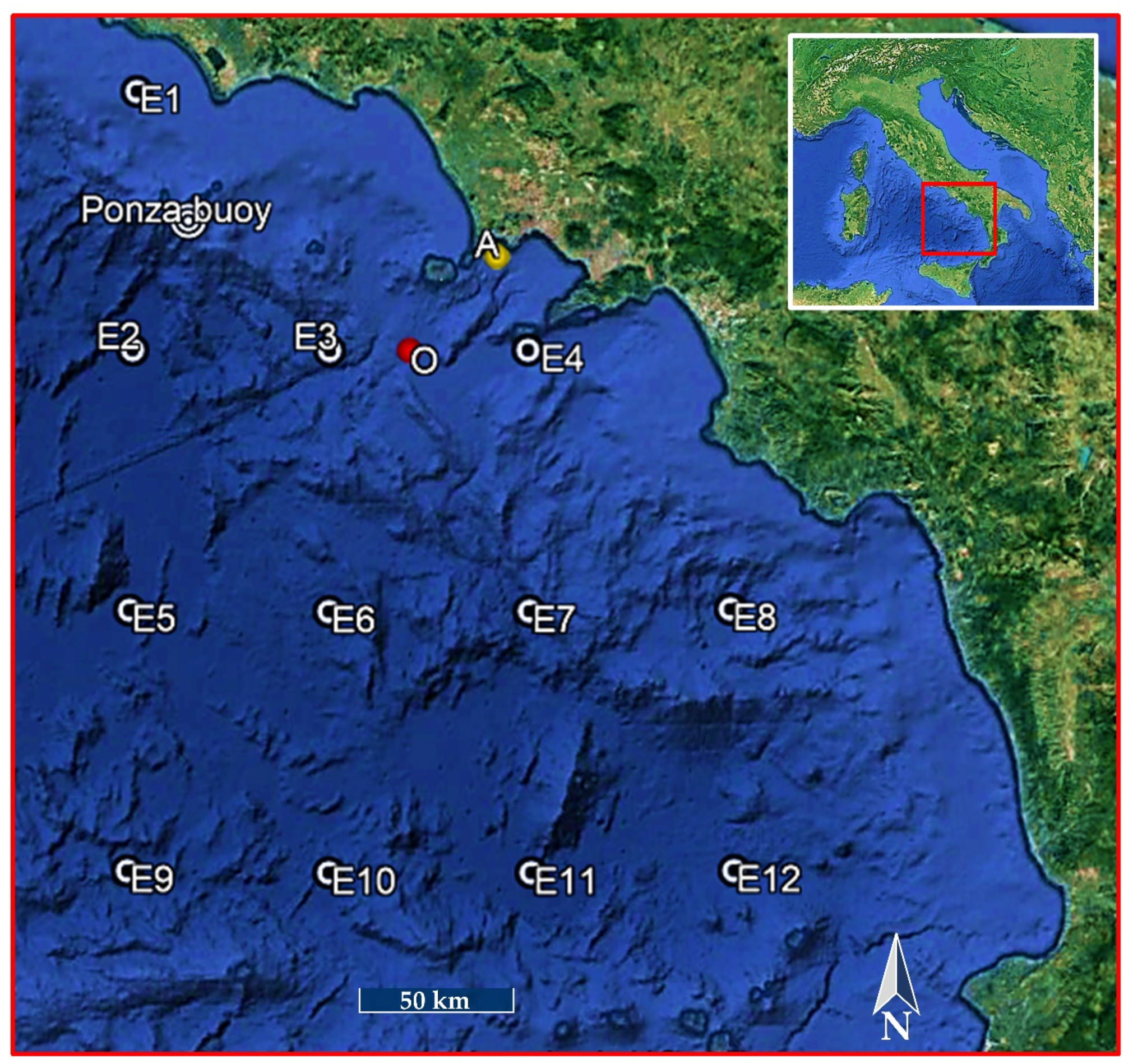
• the spatial resolution, the Italian Wave Network (IWN) consisting of only 15 stations positioned along the more than 7000 km of Italian coasts [6];
• the temporal window, since the oldest buoy of the IWN in operation from 1989 until 2014 [1,7].

As result, nowadays, ECMWF, which covers the period from 1 January 1979 onward and continuously extends forward in near real time, is assumed as the only source for wave climate assessment [8,9,10,11,12,13,14]. Several papers have discussed how to validate hindcast data (e.g., [15,16,17,18,19,20,21,22,23,24]). For coastal engineers and marine scientists, it is important to take into account the tendency to underestimate significant wave height values during severe storm conditions performed by the ECMWF dataset, as evidenced in several studies [6,8,25,26,27,28,29,30,31,32,33,34,35]. Biased estimates of wave heights will affect [36,37] both long-term return level estimates for extreme wave analysis and the short/medium time wave climate in nearshore areas, resulting from the wave model being forced with a hindcast dataset.

The detailed validation of the ECMWF hindcast model and coastal propagation model are beyond the scope of the present paper. The goals of this study are to:

• perform a comparison of different calibration stages based on the triple collocation method [38,39,40,41,42,43,44,45,46,47,48,49] and on the use of multiple numerical geographical domains with different orientations;
• highlight the discrepancies and errors in the use of different sources of wave data for both offshore and nearshore wave climate analysis from the perspective of coastal engineering measures and especially in the assessment of non-extreme wave conditions.

The latter are of particular importance for the study site, the Bagnoli-Coroglio Bay, because it represents one of the most polluted areas in the world but is nestled between two marine protected areas (the Gaiola and the Baia marine protected areas). This large bay at the north-western end of the Gulf of Naples (Tyrrhenian Sea) is included within the contaminated Sites of National Interest (SIN) for the high levels of environmental contamination by heavy industrial activities by the Ilva, Eternit, Cementir and Federconsorzi industrial factories and plants [50,51]. Due to the limited exchange of water, the accumulation of pollutants poses major concerns for human and environmental health [52]. In 2015, the Italian central government took over the planning competences over the area. By the end of 2015, the remediation of soil surfaces and the marine area has not yet been completed. In the former industrial area, most of the buildings have been demolished, while the surface and subsoil have been remediated by only 50%. In the southern portion of the area, which hosted the asbestos industry, only 30% of the remediation has been completed [53]. In the period of 2016–2018, researchers collected updated information to develop the next phase of the restoration project. This research phase was granted by the ABBaCo project (“Sperimentazioni pilota finalizzate a restauro Ambientale e Balneabilità del SIN Bagnoli-Coroglio”) [54,55], in which the present study takes form.

In addition to wave data for both littoral drift/shoreline modeling, future wave climate assessment should include other detailed eco-hydraulic analyses in order to respond to the nascent requests of marine biologists and ecologists (e.g., the coupled turbulence-dissolved oxygen dynamics modeling and forecasting, [56]; projected changes in wave climate [57,58], nearshore velocity field and related dynamics of deep chlorophyll [59,60,61,62,63], habitat mapping purposes [64,65,66,67,68] and ecosystem-based coastal defence [69,70,71,72,73]). Therefore, results from a high-resolution coastal propagation model have been compared with the in situ measurements of an innovative economical GPS-based wave buoy and with an acoustic Doppler current profiler (ADCP) in order to calibrate the numerical model itself. The measurements have been carried out by placing the pair of instruments very close to each other. In particular, a wave buoy called the directional wave spectra drifter, (DWSD) designed and fabricated by the Lagrangian Drifter Laboratory (LDL) of the Scripps Institution of Oceanography (SIO) [74], is examined, exploring its significant potential use in a low-cost drifter for measuring waves in coastal areas.

1.2. Approach and Challenges

The triple collocation—DWSD buoy, ADCP and virtual numerical point—makes possible an implicit validation between instrumentations and between instrumentation and numerical model. Considering the recent depletion of the IWN, as well as in all of Europe, mainly due to the high costs of maintenance of the traditional wave buoy systems, the opportunity to develop cost-effective and sustainable technologies to monitor waves is of strong interest to researchers and engineers. In the last decade, global positioning system (GPS) technology has been introduced in wave buoys as a cheaper alternative to traditional instruments which mainly utilized accelerometers to measure the pitch, heave and roll of the buoy [75,76,77,78,79,80].

Technological advancements of the GPS receivers have helped the development of reliable GPS-tracked wave buoys, which are currently gradually complementing conventional sensor-based wave buoys, offering the same high-quality data as traditional, well-established, accelerometer-based buoys such as the Datawell directional wave-rider buoys [81,82,83,84,85,86,87,88,89,90,91,92,93]. GPS technology has also been largely adopted in the development of surface drifters that track the world ocean surface circulation [86,87,88], while other authors [89,90,91] have recently proposed that the GPS drifter is particularly suited for nearshore or surf-zone applications. The use of a GPS receiver, as opposed to an autonomous instrument package, results not only in considerable cost saving but it enables also the development of smaller buoys, which can be easily transported, deployed and handled from a small boat. This wave buoy has been developed, moving on from the experience acquired from the Global Drifter Program (GDP) [86,87,88,89]. Its small size (40-cm diameter) also has the advantage of coping with a higher wave frequency, extending the range of measurement [93].

The idea to have multiple lines of evidence agree has always fascinated climate scientists and ocean modelers, and a cluster of wave buoys goes right in that direction. Therefore, this work describes an experience of a calibration procedure in which multiple numerical simulations, called ensembles, are calibrated by means of the DSWD buoy.

The method presented in this work allows an enclosing calibration procedure to be a building block in a single two-step approach. The triple collocation technique (applied in a point outside the study area) has been used solely to provide a first “rough” calibration. Having this fast calibration (first step), then (second step) the tuning of wave parameters in the numerical model, is refined by an ensemble of five numerical domains running in different wave sectors, in which time series are compared with another DWSD buoy located within the study site. Finally, we demonstrate the method via direct comparison with the wave time series measured by an ADCP installed in the bay. The final dataset obtained from the calibrated model has been used to describe the local wave climate. Quali-quantitative considerations from the whole historical dataset are drawn. The results suggest that the numerical model’s calibrations, based on short-term wave buoy measurements, can be easily applied in different areas where detailed wave data are not available.

The paper is organized as follows: the next section provides detailed information on the hindcast model and the instruments used at the study site, as well as a description of the numerical model and the underpinning assumptions that were used to carried out the calibration. In Section 3, the validation results of the DSWD buoy against the ADCP are reported. Moreover, the final dataset obtained from the calibrated model has been used to describe the local annual wave climate. Sources of uncertainty, relevant shortcomings and contradictions between the calibrated and uncalibrated numerical model are also highlighted. Section 4 is devoted to an overall discussion, with remarks on the future perspective. Finally, some conclusions are drawn.

2. Wave Data and Methodology

2.1. Offshore Wave Dataset

The present work has been based on two sources of offshore wave data: wave buoy records and hindcast data. The first have been supplied by pitch-roll type directional buoys operating offshore in Ponza (central Tyrrhenian Sea). The records are available from 1 July 1989 [94,95], as a part of the IWN. From 1989 to about 2002, the wave buoys collected 30 min of wave measurements every 3 h, but when in the presence of wave heights greater than 1.5 m, the measurements were continuous. From 2002 to 31 December 2014, the wave measurements were always continuous and the wave characteristic parameters refer to 30-min time intervals. In any case, the dataset comprises the spectrum zero-moment wave height (H_m0), the mean wave period (T_m) and the mean wave direction (θ).

A gross stochastic error detection phase has been applied. The data processing has firstly regarded the missing data problem. Missing values reduce the representativeness of the sample and they can severely disturb the conclusions drawn from the data. For Ponza buoys, about 10% missing data, covering about 20 years of observation, have been detected. In order to get a conservative estimation in case of a lack in the time series, missing data or values of wave height of less than 0.2 m for several hours have been considered as errors and removed. However, to test the sensitivity of the results, H_m0 = 1 m and 2 m have also been used. This analysis has shown that the estimated wave energy flux does not differ substantially (i.e., less than 12%) if wave heights of 1 m or 2 m are used to fill the missing data. Therefore, by considering missing data, unrealistic calm conditions and spikes, of the approximately 126 thousand available data of the whole dataset, only 96,879 values were considered useful.

In addition to these buoy records, the dataset was compared/complemented with the ECMWF dataset [4], in which historical observational data spanning an extended period are implemented through a single consistent analysis in forecast models. The ECMWF dataset is composed of a coupled ocean atmosphere and a general circulation model, i.e., an atmospheric reanalysis coupled with a wave model integration where no wave parameters are assimilated, making the wave part a hindcast run.

The dataset used is termed ERA-Interim, continuously updated in real time. Significant wave height (H_m0), mean period (T_m) and mean direction (θ), ranging from January 1979 to December 2018, were extracted from the ERA-Interim archive, available for download online [46].

The ECMWF internal WAve Model (WAM) covers the Mediterranean Sea by a base model grid with a resolution of 0.75° × 0.75°. ERA-Interim and WAM products are publicly available on the ECMWF Data Server. The WAM provides wave characteristics assimilated every 6 h. Here, 12 grid points (E1–E12) were considered. The geographical coordinates and distance from the seabed of all offshore points that are of interest to the present study are shown in

Table 1. Geographical information of ECMWF grid points E1–E12, Ponza wave buoy and reference point O (offshore of the Gulf of Naples) and point W (offshore Pozzuoli’s Gulf).

Point	Latitude	Longitude	Depth
E1	41.25 N	12.75 E	122
E2	40.50 N	12.75 E	3601
E3	40.50 N	13.50 E	1688
E4	40.50 N	14.25 E	1017
E5	39.75 N	12.75 E	3591
E6	39.75 N	13.50 E	3072
E7	39.75 N	14.25 E	2377
E8	39.75 N	15.00 E	1755
E9	39.00 N	12.75 E	3020
E10	39.00 N	13.50 E	3179
E11	39.00 N	14.25 E	3438
E12	39.00 N	15.00 E	2781
Ponza buoy	40°52′0.10″ N	12°57′0.00″ E	100
O	40°29′45.06″ N	13°47′46.70″ E	1037
W	40°45′56.49″ N	14° 7′41.22″ E	100

. The position of point O, as representative of the “offshore” of Gulf of Naples, and of point W (offshore Pozzuoli’s Gulf), are also reported. Geographical information is graphically represented in Figure 1.

2.1.1. Comparison of Offshore Wave Data

The assessment of the whole dataset available for the Ponza wave buoy and for ECMWF time (point E3) is graphically represented with polar diagrams assembled in Figure 2. The wave dataset obtained from the Ponza wave buoy by means of the “geographic transposition of wave gauge data” to point O is also reported. The geographic transposition has been applied according to the method originally formulated by Contini and De Girolamo [96].

The method is based on the following hypotheses:

(a)

the wind speed and direction are the same at both real and “virtual” (transposed) stations;

(b)

the extent of the wave generation region can be described by the effective fetches [97];

(c)

the wind blows over the fetch long enough to assume that wave conditions are independent of the wind duration (fetch-limited conditions);

(d)

both real and virtual stations are in deep water.

Under the above conditions, the spectral significant wave height H_m0 and the peak period T_m can be estimated using the Sverdruv Munk Bretschneider (SMB) method [98]:

$$\frac{g\times H_{m0}}{U_A^2}=1.6\times {10}^{-3}\times {\left|\frac{g\times F}{U_A}\right|}^{\frac{1}{2}}$$

(1)

$$\frac{g\times T_m}{U_A^2}=2.857\times {10}^{-1}\times {\left|\frac{g\times F}{U_A}\right|}^{\frac{1}{3}}$$

(2)

where g is the gravity acceleration, U_A represents the wind-stress factor and F is the effective fetch.

Equations (1) and (2) can be written at real and virtual sites and, under the assumption that wind conditions are the same for both stations, the following equations can be derived:

$$\frac{H_{m0,V}}{H_{m0,R}}={\left|\frac{F_V}{F_R}\right|}^{\frac{1}{2}}=K_H$$

(3)

$$\frac{T_{m,V}}{T_{m,R}}={\left|\frac{F_V}{F_R}\right|}^{\frac{1}{2}}=K_T$$

(4)

where the subscripts R and V denote the variables referring to the real and virtual station, respectively.

The “transposition coefficients” K_H and K_T allow us to calculate from the real wave buoy records the transposed wave gauge dataset at the virtual station. For the sake of completeness, the virtual station O was selected between the ECMWF grid points E3 and E4 before the hindcast data analysis. In this way, once we selected the best ECMWF reference point from one of the two points, a sufficient comparison with the transposed dataset was ensured. More than 65% of the annual wave energy comes from the sector 220°–280°, in accordance with the long fetch facing the Gulf and with the mesoscale climate conditions, with swells approaching from distant storms coming from the NW sector of the Mediterranean Sea.

The comparison between the ECMWF dataset and buoy records (both real and transposed) shows some differences. In particular, the rate of waves coming from the east is significantly reduced. Then, the lowest values of energy in the ECMWF points are noticeable, particularly in the highest power class. It can be seen that the average wave power moves from 3.85 kW/m computed at the Ponza wave buoy (4.73 kW/m for point O) to 2.19 kW/m at point E3 (

Table 2. Main wave climate parameters (based on the whole datasets) at Ponza wave buoy, point O and ECMWF grid point E3.

Dataset	Hs,mean	Hs,max	σH	Tp, mean	Tp, mean	σT	θm	σθ	P,mean
	(m)	(m)	(m)	(s)	(s)	(s)	(°)	(°)	(kW/m)
Ponza buoy	0.89	7.9	0.71	5.49	33.33	2.34	215.92	70.95	3.85
Point O	0.92	9.46	0.79	5.63	38.16	2.49	215.92	70.95	4.73
E3	0.65	6.133	0.53	5.07	11.54	1.44	222.62	76.51	2.19

).

Moreover,

Table 3. Average differences between the buoy records (at Ponza and transposed at point O, respectively) and ECMWF hindcast data for point E3.

Hs (m)	Hs,PONZA BUOY/Hs,ECMWF (m)	Hs,POINT O/Hs,ECMWF (m)
<0.5	1.04	1.06
0.5–0.75	1.75	1.77
0.75–1	1.47	1.50
1–2	1.41	1.43
2–3	1.35	1.37
3–4	1.21	1.36
Mean	1.37	1.42

shows the average differences between the measurements carried out by the buoy (at Ponza and after transposition at point O, respectively) and the hindcast data. Such values of H_{s,PONZA BUOY} / H_s,ECMWF and H_{s,POINT O} / H_s,ECMWF are organized by wave class (in terms of H_s ranges).

It is possible to note that for calm conditions (H_s < 0.5 m), the datasets are very similar. The highest discrepancy was found for 0.5 m < H_s < 0.75 m, where values of H_s recorded by the Ponza wave buoy (point O, respectively) were on average 1.75 times (1.77, respectively) higher than those reported for the E3 hindcast data. The overall mean discrepancy between the Ponza buoy and the ECMWF data was 1.37, while between point O and ECMWF, it was 1.42. A comparison of the wave height time series obtained from the different datasets is highlighted in Figure 3.

The bulk of these differences can be attributed to the dissimilar measurement conditions. The smaller sampling frequency for the hindcast data involves peak attenuation, acting as a band-pass filter and smoothing the signal. The underestimate of the ECMWF data was previously highlighted within the WW-Medatlas projects [28]. Moreover, through intercomparison with NCEP (National Centers for Environmental Prediction) Climate Forecast System Reanalysis [26] and with wave buoy data, the lowest values of energy in the ECMWF points were detected, especially in the highest power class (e.g., [6,10,27,36]). Hence, the use of the ERA-Interim dataset could be considered adequate for slightly conservative wave power potential and studying long-term variations in wave height [10] but, at the same time, should be examined carefully during detailed resource assessments or for arriving at the design wave condition or to build a detailed nearshore wave model. The main parameters of the wave climate at each grid point are reported in

Table 4. Main wave climate parameters (based on 39-year average) at ECMWF grid points.

Point	Hs,mean (m)	Tm, mean (s)	θ, mean (°)	Pmean (kW/m)
E1	0.64	4.43	222.63	2.19
E2	0.77	4.71	229.82	2.94
E3	0.65	4.43	222.62	2.19
E4	0.67	4.55	237.02	2.49
E5	0.85	4.86	235.25	3.77
E6	0.79	4.83	237.98	3.69
E7	0.74	4.69	242.95	2.91
E8	0.69	4.68	240.89	2.56
E9	0.95	4.87	238.58	4.73
E10	0.95	4.87	238.59	4.11
E11	0.86	4.72	249.12	4.11
E12	0.75	4.70	254.91	3.13

.

A tentative contour map (based on interpolation of power rate at 12 grid points) has been provided in Figure 4, where wave power isolines are depicted, ranging from 2.5 to 5 kW/m.

2.2. Study Site and Nearshore Wave Instrumentation

The nearshore study site is represented by the Bagnoli-Coroglio Bay, located within the Gulf of Naples, a natural semi-enclosed embayment within the Gulf of Pozzuoli (also known as the Gulf of Puteoli). Its mean depth is ca 60 m, with a maximum depth of 110 m and a surface area of 33 kmq.

Due to the proximity to the city of Naples, the whole area historically represents one of the best studied coastal areas of the Mediterranean Sea [99].

Thanks to the presence of the Stazione Zoologica “Anton Dohrn” (SZN) since 1872, marine investigations have been carried out for more than a century and half [100]. Recently, two Monitoring and Environmental Data Units (MEDA) of the SZN have been installed in the Gulf of Naples and in the Gulf of Pozzuoli (Figure 5). These MEDA units are mainly used for the chemical, biological and environmental monitoring of the marine ecosystem and both are equipped with an ADCP [61]. This shallow marine area is also famous, as it is the most highly active volcanic district in the coastal zone of SW Italy [101]. The geographical coordinates and water depth for MEDA A (Gulf of Pozzuoli) and MEDA B (Gulf of Naples) are indicated in

Table 5. Geographical information of MEDA units.

Point	Latitude	Longitude	Depth
MEDA A	40°49.668’ N	14°13.984’ E	19.0
MEDA B	40°48.550′ N	14°09.300’ E	17.5

. Close to MEDA B, a DWSD wave buoy (DWSD-B hereafter), provided by the University of Campania, was installed during a field campaign which took place from May to June 2016 [93]. Instead, in the period of February–March 2017, a DWSD buoy (DWSD-A) was placed close to MEDA A.

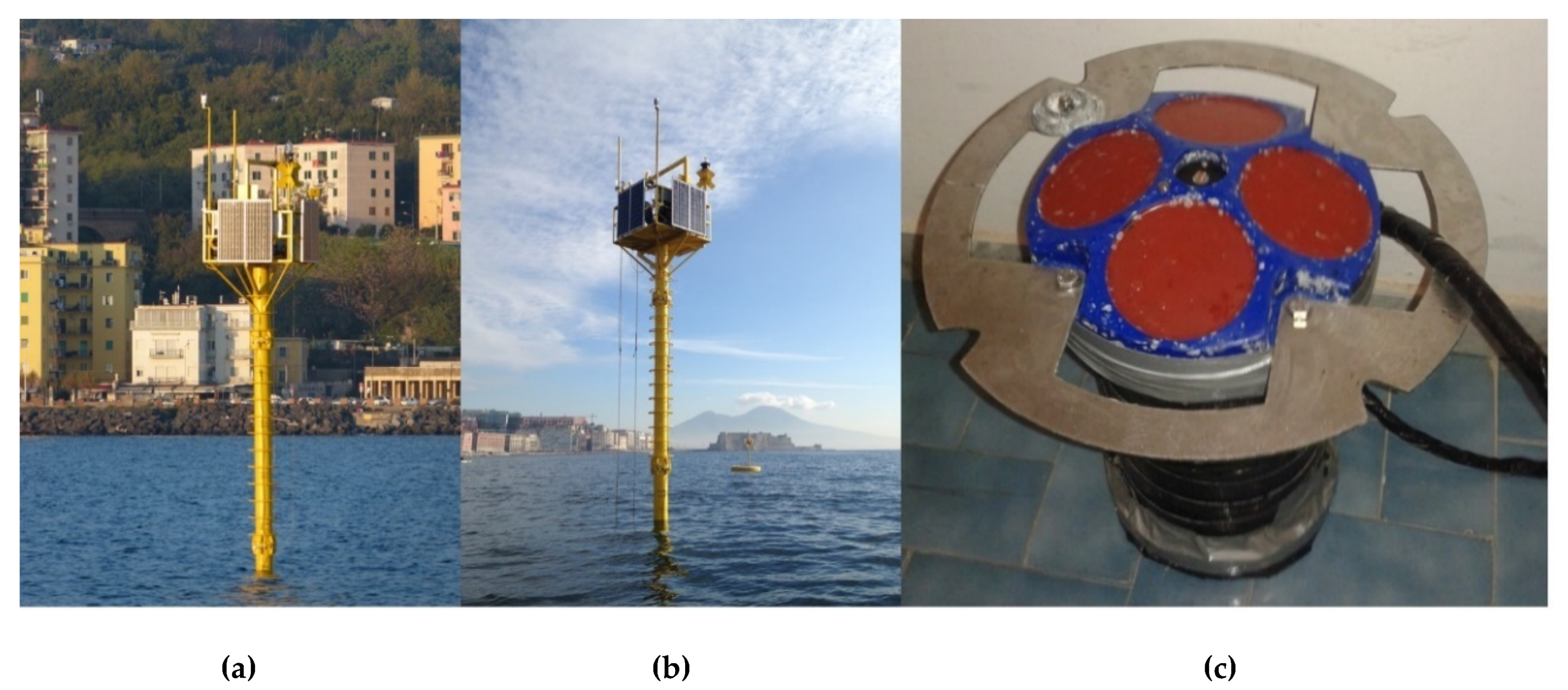
2.2.1. Acoustic Doppler Current Profiler

The ADCPs used for the test campaign are one of the most widely used instruments in oceanographic research for measuring the wave velocity profile. Such instruments are also able to provide wave information. ADCP-A and ADCP-B are part of the aforementioned MEDA A and MEDA B, respectively. The ADCP (Figure 6) is a bottom-mounted upward-looking instrument which takes the measurements of the waves basically using three independent techniques.

The first method is wave measuring using the basic principle of Doppler shifting to evaluate the orbital velocities of waves, ensonifying the entire water column along four inclined beams. The orbital velocity measured by the ADCP along each distant beam provides information above the directional and non-directional wave spectrum. In addition to wave orbital velocity measurement, the ADCP also measures the non-directional spectra through echo ranging (surface track) and bottom pressure with a pressure transducer, providing redundant measurements of wave height and water depth.

In

Table 6. ADCP configuration.

Time between Full Ensemble Records	(15 min)
Frequency	(600 kHz)
Size of the depth cell	(50 cm)
Number of bins in the current profile	(49 bins)
ADCP altitude above bottom	(50 cm)
Number of beams	(4 beams)

and

Table 7. The spectral analysis parameters of the ADCP.

Frequency band width	(0.0078 Hz)
Maximum upper cutoff frequency	(0.5 Hz)
Sea-swell transition frequency	(0.11 Hz)
Minimum lower cutoff	(0.039 Hz)
Number of direction frequency bands	(128 bands)
Number of frequency bands	(128 bins)

, the ADCP specification and the parameters used for the spectral analysis are described. Details of the ADCP wave measurements are described in [102,103,104,105,106].

2.2.2. Directional Wave Spectra Drifter-Derived Wave Buoy

The DWSD buoy uses the GPS sensor package in order to measure w(t), u(t) and v(t), which represent respectively the vertical, horizontal E-W and horizontal S-N buoy velocity components, from changes in the frequency of the GPS signal [86,93,107,108]. The measurements are made for a 17 min long sample of u(t), v(t) and w(t) every hour, divided into overlapping 4-min segments with 1 Hz of sampling frequency. The power spectral density, co-spectra and quadrature-spectra parameters are derived from a Fourier transform of the correlation functions related to each pair of the three aforementioned signals, giving the first five independent Fourier coefficients (a₀, a₁, a₂, b₁, b₂) and thus the wave spectra for each hourly sea state. For each measured sea state, the three velocity components, the computed first five Fourier coefficients and the main wave data parameters are transmitted in real time through the Iridium satellite system. All these wave data, including data on battery voltage and the pressure, temperature and humidity of the hull, are accessible in real time from a dedicated website.

The DWSD buoy (Figure 7) has a simple spherical geometry with a diameter of 0.39 m and weight of 12 daN, reducing in this way the installation and maintenance costs, being very easy to handle and to install.

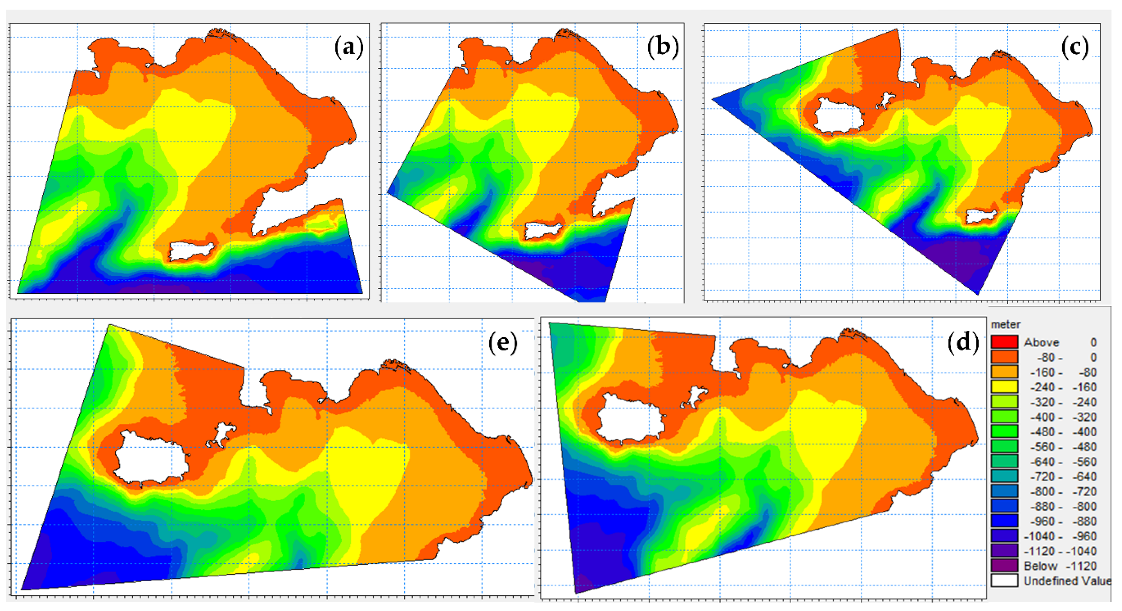
2.3. Wave Propagation and Model Calibration

In order to consider the intricate variations in wave energy density occurring from offshore of the Gulf of Naples to the Bagnoli-Coroglio Bay, the nearshore energetic patterns have been studied by means of the numerical suite MIKE 21 SW spectral wave model, developed by DHI Water and Environment [109]. The model takes into account the effects of refraction and shoaling due to varying depths and local wind generation and energy dissipation due to bottom friction and wave-breaking, and it has been validated by comparison with data from buoys and satellites by several authors [8,110,111,112,113]. Moreover, several scientific papers (e.g., [114,115,116,117]) discussed the overall satisfactory agreement between MIKE 21 SW and SWAN, TOMAWAC and STWAVE. In particular, Ilia and O’Donnell [118] found that both MIKE 21 SW and SWAN were largely consistent in their observations during storms, even if MIKE 21 SW predicted some of the storm peaks slightly better than SWAN. Therefore, the results from this study can be of interest for applications with other spectral wave models.

The basic equations in the model are derived from the conservation equation for the spectral wave action density Z, based on the approach proposed by the authors of [119]. In fact, in the presence of currents, wave action is conserved whilst the wave energy is not [120]. The source/sink term that represents all physical processes which generate, dissipate or redistribute energy, S_tot, can be written as:

$$S_{tot}=S_{in}+S_{surf}+S_{dw}+S_{bot}+S_{nl}$$

(5)

where S_in represents the energy transfer from wind to waves, S_surf is the dissipation of wave energy due to depth-induced breaking, S_dw is the dissipation of wave energy due to whitecapping, S_bot is the dissipation due to bottom friction and S_nl is the energy transfer due to non-linear triad (three-wave) interactions. The following approaches/models are used in the model:

• for the wave bathymetric breaking, the formulation proposed by Battjes and Janssen [121];
• the formulation of Kofoed-Hansen and Rasmussen [122] for bottom friction dissipation;
• the Komen et al. [123] dissipation model for whitecapping;
• the triad-wave interaction is modeled using the simplified approach proposed by Eldeberky and Battjes [124,125];
• for Snl parameterization, the discrete interaction approximation developed by Hasslmann et al. [126].

Operatively, the models compute the evolution of Z by solving the action balance equation [127], which in the Cartesian co-ordinates can be written as:

$$\frac{\partial Z}{\partial t}+{\nabla }_{x,y}\left[\left(C_g+U\right)Z\right]+\frac{\partial }{\partial \sigma }\left(C_{\sigma }Z\right)+\frac{\partial }{\partial \theta }\left(C_{\theta }Z\right)=\frac{S_{tot}}{\sigma }$$

(6)

where Z = V/σ, V being the variance density and σ the relative angular frequency, θ is the mean wave direction measured clockwise from true north, C_g is the group velocity, U is the current velocity vector and C_σ and C_θ are the propagation velocities in spectral space (σ,θ). The left-hand side of the above equation represents the local rate of change of the wave energy density, propagation in geographical space and shifting of frequency and refraction due to the spatial variation of the depth and current.

For wave propagation over slowly varying depths h, σ can be written by means of the linear dispersion relation

$$\sigma =\sqrt{g k tanh\left(kh\right)}$$

(7)

in which k is the wave number.

The magnitude of the group velocity C_g is given by

$$C_g=\frac{\partial \sigma }{\partial k}=\frac{1}{2}\left[1+\frac{2kh}{\sin \mathrm{h}\left(2kh\right)}\right]\sqrt{\frac{g}{h}\tan \mathrm{h}\left(kh\right)}$$

(8)

The implicit assumption of these equations is that properties of the medium (water depth and current) as well as the wave field itself vary on time and space scales that are much larger than the variation scales of a single wave.

The model takes into account diffraction by using the approximation proposed by Holthuijsen et al., [128], based on the revised version of the mild slope equation model of Berkhoff [129] that was proposed by Porter [130].

It is worth noting that the source functions S_in, S_nl and S_ds in MIKE 21 SW are similar to the source functions implemented in the WAM Cycle 4 model [131,132]. The latter provides the basis for the ECMWF wave hindcast dataset [16,133,134]. One of the main restrictions of the model is that when propagation leads to waves moving nearly parallel and close to the coast, there is an unrealistic loss of energy caused by the large second-order diffusion error [135]. In this case, moreover, the main assumption that the source integration time step has to be shorter than or equal to the propagation time step is at fault. Hence, an intrinsic sensibility to direction can be detected, representing a warning if significant diffraction-reflection conditions can be found.

The model solves the governing equation by means of finite element-type methods to discretize geographical and spectral space. A parameterization of the conservation equation in the frequency domain is performed by introducing the zeroth and the first moment of the action spectrum as dependent variables.

The computational domain was discretized using an unstructured grid with meshes based on linear triangular elements (Figure 8) and performed using the cell-centered finite volume method. The seabed was performed by interpolating at the grid nodes the information provided by the General Bathymetric Chart of the Oceans (GEBCO) database [136]. The grid resolution was assumed to be variable linearly between the maximum depth to 150 m for depths in the range of 500 m to 100 m. Constant values of 150 m and 1000 m of the grid resolution have been assumed for water depth shallower than 100 m and deeper than 500 m, respectively.

The wave model was run as forced wave-by-wave with data from the ECMWF internal WAve Model (WAM) with the ERA-Interim dataset related to source point E3. The basic data necessary to fulfill the offshore requirements are the significant wave height (H_m0), mean wave period (T_m) and mean wave direction (θ), provided by 6-h hindcast wave data. Wave power series was calculated from the resulting dataset provided by the transformation model. For natural sea states, where waves are random in height and period (and direction), the spectral parameters have to be used. The wave energy flux can be defined as:

$$P=\rho g{\displaystyle {\int }_0^{2\pi }{\displaystyle {\int }_0^{\infty }{C}_g(f,h)S(f,\theta )dfd\theta }}$$

(9)

where ρ is the sea water density, S(f,θ) denotes the 2D wave spectrum as a function of the spectral wave frequency f and mean wave direction θ and C_g(f,h) denotes the wave group velocity, expressed by Equation (8).

2.3.1. First Step: Triple Collocation

Although a phase-decoupled approach is employed in order to reproduce the qualitative behavior of changes and spatial redistribution in the wave direction, when significant diffraction conditions are detected (e.g., in front of reflecting obstacles like rocky coasts), a Boussinesq-type model is required. However, due to the large extension of the spatial domain and the large wave dataset and computing effort normally required for the computation of diffraction in arbitrary geophysical conditions, a different approach was applied in the present study. Taking into account the way in which MIKE 21 SW solves the equations, better results are normally obtained with waves that are parallel to one of the coordinate axes or (if just one boundary is used to force the model) perpendicular to the offshore boundary from which the input waves are coming [137]. Therefore, the input open boundary should be placed so that the main wave direction is orthogonally aligned. Looking to a large scale, the exchanges between the Gulf of Naples and the Tyrrhenian Sea occur along the Bocca Grande, the main aperture of the gulf between Ischia and Capri. Considering that Bocca Grande opens to the west into the Mediterranean Sea and the bulk of the waves are provided by westerly waves [5], firstly, the open boundary of the numerical domain was orthogonally aligned along the 220° N direction. For convenience, we will call this domain M220°. Under this domain, the numerical model was forced with the hindcast data by ECMWF (grid reference point E3). Since two sources of direct meausurement of the “physical truth” (with certain systematic deviations and random errors) are available (i.e., ADCP-B and DWSD-B datasets), the search for the best set of model parameters (breaking parameter, bottom friction and white capping) was iteratively obtained by firstly applying a triple collocation procedure. This is the singularity of the present study, for which the third dataset is not univocally defined: the triple collocation is not used just for error estimation purposes but to help the search for the best calibration.

The term “triple collocation” indicates a methodology used to characterize systematic biases and random errors in satellite observations, model fields and in situ measurements. It attempts to segregate the measurement uncertainties, spatial and temporal representation and sampling differences in the different datasets by an objective method [137,138]. A frequent and often biased assumption is that all errors are due to the system that is being tested against a reference system, that is in turn assumed perfect. In this vein, Stoffelen [38] also refers to the biases associated with regression and with error distributions. These issues cannot be clearly resolved in dual comparisons, as scatter will be caused simultaneously by all the above issues for both observing systems, and there is no clear objective way to assign errors to one or the other [139]. In triple collocation, instead, three (ideally) independent datasets are brought together, so that three scatter plots can be made. Focusing on the specific application to coastal engineering, and referring to studies provided by Robertson et al. [45], Muraleedharan et al. [42] and McColl et al. [46], the technique needs the assumption of a linear relationship between the measured value and true value. The following equation can be considered:

$$X_i={\alpha }_i+{\beta }_{i}T+e_i$$

(10)

where the Xi (i ∈ {1, 2, 3}) are collocated measurement systems linearly related to the true underlying value T with additive random errors e_i, respectively. The terms α_i and β_i are unknown calibration parameters representing bias and the linear calibration coefficient (i.e., the ordinary least squares intercepts and slopes, respectively).

Given that the true value T is unknown, this method requires that one of the datasets is defined as the reference. However, as noted by Janssen et al. [40], the choice of T does not affect the results. The ADCP-B dataset was defined as the reference dataset; hence, its α and β will be set to 0 and 1, respectively.

The first step removes α from the datasets by introducing the following new variables:

$$X_i^{\prime }=X_i-{\alpha }_i$$

(11)

A new set of equations, without T, result from inserting (11) into (10). The uncertainty term e in (10) can be modified to:

$$X_i^{″}-T=\frac{X_i^{\prime }}{{\beta }_i}-T=\frac{e_i}{{\beta }_i}=e_i^{″}$$

(12)

By calculating the difference between any two of above equations, the true value can be eliminated, obtaining the following:

$$X_1^{″}-X_2^{″}=e_1^{″}-e_2^{″}$$

$$X_3^{″}-X_2^{″}=e_3^{″}-e_2^{″}$$

(13)

$$X_1^{″}-X_3^{″}=e_1^{″}-e_3^{″}$$

Assuming the errors from the independent sources have zero mean and are uncorrelated with each other and with T, error terms can then be calculated by multiplying any of the two equations above, introducing the mean values:

$$\overline{(X_1^{″}}-\overline{X_2^{″}})\left(\overline{X_3^{″}}-\overline{X_2^{″}}\right)=\left(e_1^{″}-e_2^{″}\right)\left(e_3^{″}-e_2^{″}\right)={\left(e_2^{″}\right)}^2$$

$$\overline{(X_1^{″}}-\overline{X_3^{″}})\left(\overline{X_2^{″}}-\overline{X_3^{″}}\right)=\left(e_1^{″}-e_3^{″}\right)\left(e_2^{″}-e_3^{″}\right)={\left(e_3^{″}\right)}^2$$

(14)

$$\overline{(X_1^{″}}-\overline{X_3^{″}})\left(\overline{X_1^{″}}-\overline{X_2^{″}}\right)=\left(e_1^{″}-e_3^{″}\right)\left(e_1^{″}-e_2^{″}\right)={\left(e_1^{″}\right)}^2$$

Then, according to Janssen et al., [40], it is possible calculate the linear calibration coefficient for the X₂ and X₃ datasets (the DWSD-B datasets and the numerical output, respectively, in the present study). It can be calculated as:

$${\beta }_2=\left(-B_2+\frac{\sqrt{B_2^2-4A_2{C}_2}}{2A_2}\right)$$

(15)

$${\beta }_3=\left(-B_3+\frac{\sqrt{B_3^2-4A_3{C}_3}}{2A_3}\right)$$

(16)

where A₂ $=r_2\overline{X_1^{\prime }{X}_2^{\prime }}$, $r_2=\overline{e_1}/\overline{e_2}$, $B_2=\overline{X_1^{\prime }{}^2}-r_2\overline{X_2^{\prime }{}^2}$, $C_2=\overline{X_1^{\prime }{X}_2^{\prime }}$, and A₃ $=r_3\overline{X_1^{\prime }{X}_3^{\prime }}$, $r_3=\overline{e_1}/\overline{e_3}$, $B_3=\overline{X_1^{\prime }{}^2}-r_3\overline{X_3^{\prime }{}^2}$, $C_3=\overline{X_1^{\prime }{X}_3^{\prime }}$.

Hence, the bias is calculated as:

$${\alpha }_2=\overline{X_2}-{\beta }_2\overline{X_1}$$

(17)

$${\alpha }_3=\overline{X_3}-{\beta }_3\overline{X_1}$$

(18)

assuming as initial values for the iterative method that ${\alpha }_2={\alpha }_3=0$ and ${\beta }_2={\beta }_3=1$. The iterative process ends when either of the bias, beta or error variance converge [45]. For this study, convergence was based on the error variance.

Operatively, the triple collocation procedure has been repeated several times with different numerical outputs (X₃) obtained each time after arbitrary modification of model parameters. It was assumed, in particular, that the calibration of the numerical output was achieved when the error variance estimated by means of the triple collocation between X₃ and X₂ and X₃ and X₁ were both smaller than the error variance between X₁ and X₂.

For the qualitative evaluation of the comparison results, statistical indicators such as bias and root mean square error (RMSE) were used. These parameters are defined as:

$$Bias\left(X_i,X_j\right)=\frac{1}{N}{\sum }_{n=1}^N\left(x_{j,n}-x_{i,n}\right)$$

(19)

$$RMSE\left(X_i,X_j\right)=\sqrt{\frac{1}{N-1}{\displaystyle \sum }_{n=1}^N{\left(x_{j,n}-x_{i,n}\right)}^2}$$

(20)

where $x_j$ and $x_i$ (i,j ∈ {1, 2, 3}, i≠j) indicate the wave parameters at the n-th hourly sea state, respectively, measured by the DWSD buoy, the ADCP or provided by numerical runs, and N is the total number of hourly sea states considered for the field test campaign. The notation is such that capital letters represent random variables, and lower-case letters represent realizations of random variables. We also may derive the bivariate correlations between the measurement sources as:

$$\Gamma =\frac{\mathrm{COV}\left({\mathrm{X}}_i,{\mathrm{X}}_j\right)}{{\sigma }_{X_i}{\sigma }_{x_j}}$$

(21)

obtained by defining the second-order quantities that are estimable directly from sample measurements, i.e., the covariance, COV(X_i,X_j), and the standard deviation, σ, of two datasets.

The key benefits of the first step can be summarized as follows:

• firstly, qualitative evaluations of the input time series amount to cheap and almost instantaneous forward runs of a pretrained network of direct measurements;
• secondly, fast and accurate approximations of numerical output with respect to the model parameters returns, since short recordings by DWSD-B and ADCP-B are taken into account.

These benefits, used together under the triple collocation technique, allow for an efficient rough calibration.

2.3.2. Second Step: Ensemble of Multiple Runs

The small gulf of Bagnoli-Coroglio Bay represents a sub-basin in the northwestern end of the Gulf of Naples. Water exchange occurs between Pozzuoli Bay and the Gulf of Naples through a section that is 100 m deep and 2 km wide. Considering its wave sector, in addition to M220°, the other four different offshore boundary orientations have been applied (M180°, M240°; M260°; M280°), as shown in Figure 9.

The main idea was that the model results coming from M220° can be improved by weighing the contributions of each sub-model. Hence, equal numbers of wave sectors from the whole offshore dataset have been propagated within the respective oriented model, as explained in

Table 8. Geographical information of nearshore study sites.

Name of the Model	Wave Sector
M180°	From 0° N to 190° N
M220°	From 190° N to 220° N
M240°	From 220° N to 250° N
M260°	From 250° N to 270° N
M280°	From 270° N to 360° N

. In other words, the 1-year wave time series was divided into five sub-series, collecting waves by the five directional ranges. The angular width of such wave sectors is not equal but is chosen concurrently, considering that the morphological characteristics of the bay and offshore directional wave rose.

At their first run, the set of model parameters found for M220° was considered. The procedure is synthesized in the scheme reported in Figure 10.

The whole dataset of resulting wave patterns obtained by means of the multi-domain procedure can be seen as not significantly affected by neglecting diffraction (i.e., not significantly different in comparison to adopting a diffraction model using just five scenarios along the mean five directions).

The calibration of each domain has been carried out, comparing the numerical results of a 1-year wave time series at the control point corresponding to the DWSD-A location, focusing only on waves coming from the reference wave sector. Then, the search for the optimal tuning parameters was carried out iteratively.

Concerning this iterative operation, it is of significative importance that an enhancement factor is introduced into the input series. In fact, after a first run for all the five boundary orientations, a sort of large bias was detected. Even if a calibration in phase one was carried out, the gross error remained too high, especially for larger wave heights. This discrepancy was not found when the geographically transposed dataset (at point O) was used to force the numerical model. Therefore, in order to use the ECMWF dataset (with the advantage of 40 years of continuous wave data), a rough correction parameter had to be applied (i.e., the enhancement factor) and then the finer calibration procedure could be applied. As previously highlighted, the use of a reanalysis product (the ERA-Interim dataset) as input for the numerical model leads to a general underestimation of the wave height. Considering that these differences can be attributed mainly to the dissimilar measurement conditions, an estimation of the discrepancies between ECMWF and IWN buoy records (the one at Ponza buoy and at point O, by transposition) is available in Section 2.1.1. In this work, the value of 1.42 (see Table 3) has been applied to amplify the wave height time series at point E3. The amplification factor was not necessary in the first step. This can be attributed to the small range of wave heights collected at MEDA B. As highlighted in Section 2.1.1, no relevant differences between reanalysis and direct measurements were detected for H_m0 < 0.75 m.

Finally, the resulting five numerical series were assembled in order to reconstruct the 1-year nearshore dataset. The main information for the assemblage was represented by the offshore wave direction provided at point E3. The logic description of the assemblage algorithm is reported in Appendix A.

3. Results

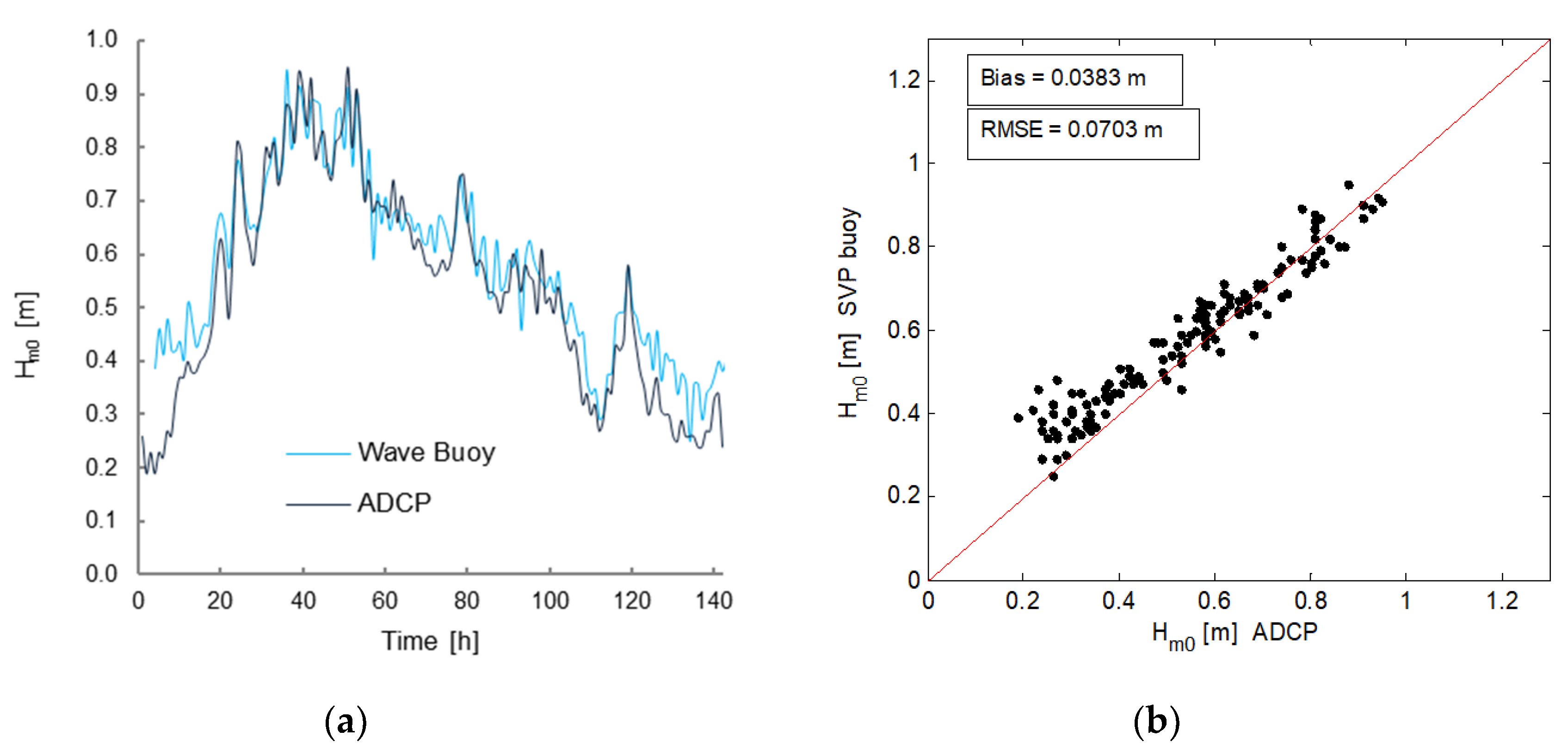
3.1. DWSD Buoy Compared to the ADCP

Figure 11a shows the time series of the significant wave height H_m0 measured by the two wave instruments, presenting very good agreement considering the very different instrumental techniques that were used. It can be noted that the time series plot between the DWSD-B and ADPC-B looks very similar, without any significant deviation, especially when the significant wave height exceeded 0.5 m. In Figure 11b, the comparative analysis of the significant wave height clearly shows a good correlation between the simultaneous buoy data and the ADCP, with a bias of 0.038 m, RMSE of 0.07 m and a correlation coefficient R of 0.96. Such a strong agreement between two wave sensors of totally different natures confirms the high quality of this cheap DWSD. For practical coastal engineering applications, sea states with values of H_m0 lower than 0.50 m are in many cases considered as calm conditions. If only the sea states greater than this threshold are considered in the comparison between DWSD and ADCP, then the results show excellent correlation, with a bias of of 0.011 m and RMSE of 0.05 m. The wave height correlation coefficient between sources is $\Gamma$ = 0.87.

The correlation of the peak period T_p between the ADCP-B and the DWSD-B is shown in Figure 12a. The peak period considered in the analysis refers to the peak related to the wind–sea spectra (0.11 Hz < f < 0.49 Hz). The results of peak periods show some small differences between the two instruments, mainly when the calculated wave spectra have multiple peaks in the wind sea frequency range (0.11 Hz < f < 0.49 Hz), of approximately equal magnitude, leading to some difficulties in the correct evaluation of the T_p. Small stochastic effects may easily modify the spectral peak, yielding a slightly different peak period. Figure 12b shows the comparison of the peak period for each sea state, showing a bias of −0.1 sec and an RMSE for the 1.1 section.

3.2. Triple Comparison

After the implicit validation between ADCP and the DWSD buoy was obtained, the M220° MIKE 21 model was calibrated. The breaking parameter, bottom friction and white capping were tuned in order to provide better wave predictions. In the present work, the iterative procedure ends when the bias related to H_s between numerical output and DWSD buoy is less than the one between ADCP-B and DWSD-B (i.e., <0.038). In particular, a bias = 0.03 m was reached.

Figure 13 shows a brief time series of the different datasets. The original ECMWF dataset (without the enhancement factor) is depicted. It is worth noting that the available data for triple comparison are few and, in particular, the range of measured wave height is between 0.4 m and about 1 m. This reinforces the need for a second stage of calibration.

It is also important to note the smoothed signal for the hindcast data and, hence, the numerical model, due to the smaller sampling frequency. By means of the small arrows in Figure 13, we also reported the offshore wave direction at point E3, which ranged between 232° N to 274° N. It can be noted that for waves coming from 230°–250° N, the numerical model fits very well with the direct measurements (in this vein, it could be seen as the envelope curve for those time series). On the other hand, when the direction became higher than 250°–255° N, the error significantly increased. This evidence corroborates the use of a multi-domain approach in order to overcome the intrinsic limits of the numerical model in relation to diffraction issues.

3.3. Final Calibration

According to the main wave direction, the five numerical domains were run. The second step of the calibration procedure was obtained by comparing the numerical output with the records at the DWSD buoy located at MEDA A. Unfortunately, during the working period of the Buoy-A, the ADCP-A did not record any data due to malfunction. A unique time series from the five datasets has been re-constituted.

Figure 14 shows the comparison between the ensemble of numerical runs as reconstituted by the five numerical domains and the Buoy-A and related to 1 year of data. This period, however, is not a consecutive time, but it was reconstituted considering the available period of measurements at ADCP-A. In other words, the fictitious 1-year ADCP-A time series was built by linking the following timeslots: 1 May 2016–30 November 2016, 1 December 2017–8 March 2018, 22 March 2017–27 April 2017. Obviously, for the numerical runs, the same temporal windows from the hindcast data were used.

The results related to 1 year are graphically represented with polar diagrams, assembled in Figure 15. The wave rose of Figure 15a shows that the 1-year predominant offshore waves are the ones coming from WNW to WSW. Depending on the system morphology, the wave rose measured at the ADCP-A (Figure 15b) undergoes a radical transformation, both in predominant direction and wave energy. The comparison between ADCP-A and wave climate obtained by using a single numerical domain (i.e., M220°, in Figure 15c) shows some differences.

The loss of directional information is noticeable for all wave height classes, resulting in an unrealistic predominant wave direction (210°–225° N): the occurrence frequency of these waves is about 48%.

The ensemble numerical runs (Figure 15d) and the energy flux from each wave class are consistent with the ADCP-A measurements and the relationship between one wave sector and another is well evidenced. As highlighted in Figure 14, the smaller sampling frequency (6-h) for the numerical model leads to lower peak values and to a reinforcement of the lowest wave height class (i.e., <0.25 m), which also occurs if the enhancement factor for the input dataset is applied. If a moving average filter (spanning 6 h) is applied to the 1-year ADCP-A measurements in order to have a time series with the same sampling frequency of the numerical ensemble, an excellent correlation can be found, with a bias of 0.009 m and an RMSE of 0.52 m. The main wave climate parameters and main statistics obtained for the various sources are reported in

Table 9. Wave statistics obtained for the various sources.

	ECMWF	Ensemble	ADCP
	Hs	Hs	Hs
	(m)	(m)	(m)
Mean	0.62	0.38	0.39
Median	0.45	0.24	0.26
Max	3.95	2.96	3.27
Min	0.07	0.00	0.00
Standard deviation	0.5	0.41	0.38
	Tp	Tp	Tp
	(s)	(s)	(s)
Mean	5.14	4.54	5.47
Median	4.94	4.55	5.4
Max	10.33	10.16	28.1
Min	1.96	0.23	0.00
Standard deviation	1.71	2.61	2.27
	θ	θ	θ
	(°)	(°)	(°)
Mean	234.39	201.7	198.65
Median	262.39	202.21	203.00
Max	359.98	359.02	359.00
Min	0.03	0.00	0.00
Standard deviation	77.07	35.99	35.72
	P	P	P
	(kW/m)	(kW/m)	(kW/m)
Mean	1.73	0.93	0.96
Median	0.4	0.09	0.13
Max	67.88	33.95	43.19
Min	0	0	0
Standard deviation	4.18	2.70	2.80

.

The results shown as the mean energy flux at MEDA A are not negligible, in contrast with the intricate morphology of the Bagnoli-Coroglio Bay.

A tentative wave energy flux density contour map is shown along the analyzed coastline in Figure 16. It is stressed that the mean wave power is able to provide its effect up to the outer surf zone. The explanation is straightforward: when the wave front is parallel to the bathymetry and, in particular, if a favourable funnel shape of the coast is recognizable, the main phenomenon governing the wave transformation is energetic refraction, and shoaling could be easily recognized as an energy-conserving, non-dissipative mechanism. This effect could in part explain the validity of the results even though a Boussinesq-type model was not used.

4. Additional Considerations and Future Perspectives

Waves are a concentrated form of solar energy. This energy flows through the Earth’s climate system, and its components respond. The response (change in energy flow) usually has impacts on other parts of the climate system. This is known as feedback. Such feedback can be positive (it leads to reinforce a small change) or negative (it acts as a stabilizing force, pushing the system back to its original state). In the context of climate assessment (also in the perspective of climate change detection), this has the opposite connotation: positive feedback destabilizes the system (which is usually bad), while negative feedback acts against the perturbation [140]. Whereas several climate factors have been classified as positive or negative feedback, storm waves and sea level rises are not univocally defined. In the study of environmental restoration projects, like the one in Bagnoli-Coroglio Bay, the identification of feedback is important in order to better understand the sensitivity of local environmental parameters to changes. The authors of [141], in analyzing the impact of sea level rises and storms along the U.S East Coast, stumbled across a variation in sea surface height associated with the Gulf Stream. As is typical of many applications, wave climate changes sit in context with internal variability and other local causes. The non-tidal condition for the Bagnoli-Coroglio area makes it possible to avoid the influence of internal modes of variability in the atmosphere. Therefore, the results of the present study may be assumed as the basis for building other models for “climate” purposes, like those for sea level rises, water circulation and heat exchange at the water surface.

A second point concerns the effectiveness of the numerical model calibration by means of a short (thus affordable and feasible) period of in situ buoy measurement. A heuristic explanation could be that the available dataset respects the hypothesis of the representativeness of the sample, i.e., it is adequate to the distribution of wave parameters. In this vein, it appears crucial that measurements cover the majority of the wave height range. The fact that measurements at MEDA A were carried out during an intense winter storm, in fact, has proven to be essential.

It is worth noting that, in the present study, a “true” triple collocation method (e.g., [39,41]) is not possible due to the short overlap of time series at MEDA-B and lack of simultaneous measurements from ADCP-A and DWSD-A.

However, the reliability of the DWSD buoy, its versatility and cost-effectiveness allows the implementation of a sustainable global array of wave sensors that will support the validation of satellite products and enhanced climatological studies, as well as providing an indispensable tool for the calibration and validation of numerical models in coastal areas.

5. Conclusions

Any eco-restoration actions require a high level of accuracy in the assessment of the nearshore wave patterns and in the definition of wave climate scenarios for the following decades. Due to this delicate issue, the accuracy and reliability of the techniques and instrumentation used to define the waves are crucial. The present study provides a non-conventional application of the multi-collocation method. In fact, essentially due to a brief overlap of sea state observations carried out by the ADCP and the DWDS buoy, a full triple collocation method is impossible to apply. However, the direct measurements available at two different locations allowed, by means of a two-step strategy, the calibration of a numerical model. In particular, during the second calibration phase, a nonparametric wave height enhancement factor was required in order to achieve the best optimization of the numerical model. The enhancement factor consists of an amplification of each value of the WAM dataset provided by ECMWF. To estimate such an amplification, it was proposed as the assumption of the average discrepancy observed between the WAM hindcast dataset at a point located offshore of the study area and the time series, obtained by the transposition of the available offshore wave buoy records. Then, the ECMWF time series was used as input for the numerical model. It was remarked that the second step used a highly representative sample consisting of measurements collected in a period experiencing a large range of significant wave height. Hence, the “need for speed” is by no means limited to rough calibration, and the path of the two-step method exposed here moves in this direction.

To summarize, two main outcomes can be considered from this study:

• the procedure here proposed, in which every sea state is subject to five (one for each grid model orientation) numerical propagations by a simpler spectral wave model, allows researchers to reach a good level of accuracy, similarly to a more time-consuming Boussinesq-type wave model which, nowadays, represents a state-of-the-art modeling technique if a very detailed wave disturbance in an enclosed coastal area needs to be explored;
• the effectiveness of numerical model calibration by means of a short period of direct measurement, opening up opportunities to use low-cost GPS buoys. To bridge the gap of abundant direct measurements in the sea from traditional wave buoy networks, the capability of GPS-buoy clusters to provide data for assimilation, calibration and validation of both climate and weather models could be optimally leveraged.

Specifically for the study area, the results shown were not negligible values of wave energy flux at the study site, also if a significant variability of punctual wave power could be envisaged. The evaluation of wave climate here presented would provide the opportunity for careful eco-engineering solutions against storm control and for restoration purposes. In this vein, it is worth noting a first application of the method to provide wave data for a source apportionment assessment of marine sediment contamination in the study area [142]. Reliable nearshore wave assessment, in fact, makes it possible to assess restoration practices from the perspective of projected medium/long term changes in sea state characteristics; for instance, those stemming from climate change (both at global and local levels). Future field campaigns will help to increase confidence in the technologies and in the approach presented in this work.

References

1. Dentale, F.; Furcolo, P.; Pugliese Carratelli, E.; Reale, F.; Contestabile, P.; Tomasicchio, G.R. Extreme wave analysis by integrating model and wave buoy data. Water 2018, 10, 373. [Google Scholar] [CrossRef] [Green Version]
2. Fortunato, A.B.; Li, K.; Bertin, X.; Rodrigues, M.; Miguez, B.M. Determination of extreme sea levels along the Iberian Atlantic coast. Ocean Eng. 2016, 111, 471–482. [Google Scholar] [CrossRef] [Green Version]
3. Franco, L. History of coastal engineering in Italy. In History and Heritage of Coastal Engineering; ASCE: Reston, VA, USA, 1996; pp. 275–335. [Google Scholar]
4. European Centre for Medium-Range Weather Forecasts. Available online: http://www.ecmwf.int/ (accessed on 10 May 2020).
5. Vicinanza, D.; Cappietti, L.; Ferrante, V.; Contestabile, P. Estimation of the wave energy in the Italian offshore. J. Coast. Res. 2011, 64, 613. [Google Scholar]
6. Vicinanza, D.; Contestabile, P.; Ferrante, V. Wave energy potential in the north-west of Sardinia (Italy). Renew. Energy 2013, 50, 506–521. [Google Scholar] [CrossRef]
7. Bencivenga, M.; Nardone, G.; Ruggiero, F.; Calore, D. The Italian Data Buoy Network. WTI Trans. Eng. Sci. 2012, 74, 321–332. [Google Scholar]
8. Contestabile, P.; Ferrante, V.; Vicinanza, D. Wave energy resource along the coast of Santa Catarina (Brazil). Energies 2015, 8, 14219–14243. [Google Scholar] [CrossRef] [Green Version]
9. Contestabile, P.; Lauro, E.D.; Galli, P.; Corselli, C.; Vicinanza, D. Offshore wind and wave energy assessment around Malè and Magoodhoo Island (Maldives). Sustainability 2017, 9, 613. [Google Scholar] [CrossRef] [Green Version]
10. Shanas, P.R.; Kumar, V.S. Temporal variations in the wind and wave climate at a location in the eastern Arabian Sea based on ERA-Interim reanalysis data. Nat. Hazards Earth Syst. Sci. 2014, 14, 1371–1381. [Google Scholar] [CrossRef] [Green Version]
11. Iuppa, C.; Cavallaro, L.; Vicinanza, D.; Foti, E. Investigation of suitable sites for wave energy converters around Sicily (Italy). Ocean Sci. 2015, 11, 543–557. [Google Scholar] [CrossRef] [Green Version]
12. Contestabile, P.; Vicinanza, D. Coastal defence integrating wave-energy-based desalination: A case study in Madagascar. J. Mar. Sci. Eng. 2018, 6, 64. [Google Scholar] [CrossRef] [Green Version]
13. Iuppa, C.; Cavallaro, L.; Foti, E.; Vicinanza, D. Potential wave energy production by different wave energy converters around Sicily. J. Renew. Sustain. Energy 2015, 7, 061701. [Google Scholar] [CrossRef]
14. Caloiero, T.; Aristodemo, F.; Ferraro, D.A. Trend analysis of significant wave height and energy period in southern Italy. Theor. Appl. Climatol. 2019, 138, 917–930. [Google Scholar] [CrossRef]
15. Sterl, A.; Komen, G.K.; Cotton, P.D. Fifteen years of global wave hindcasts using winds from the European Centre for Medium-Range Weather Forecasts reanalysis: Validating the reanalyzed winds and assessing the wave climate. J. Geophys. Res. Ocean. 1998, 103, 5477–5492. [Google Scholar] [CrossRef]
16. Janssen, P.A.E.M.; Bidlot, J.R.; Abdalla, S.; Hersbach, H. Progress in ocean wave forecasting at ECMWF. In ECMWF Technical Memory; ECMWF: Reading, UK, 2005; p. 27. [Google Scholar]
17. Palm, S.P.; Benedetti, A.; Spinhirne, J. Validation of ECMWF global forecast model parameters using GLAS atmospheric channel measurements. Geophys. Res. Lett. 2005, 32. [Google Scholar] [CrossRef]
18. Klein, S.A.; Jakob, C. Validation and sensitivities of frontal clouds simulated by the ECMWF model. Mon. Weather Rev. 1999, 127, 2514–2531. [Google Scholar] [CrossRef]
19. Molteni, F.; Buizza, R.; Palmer, T.N.; Petroliagis, T. The ECMWF ensemble prediction system: Methodology and validation. Q. J. R. Meteorol. Soc. 1996, 122, 73–119. [Google Scholar] [CrossRef]
20. Hanna, E.; Valdes, P. Validation of ECMWF (re) analysis surface climate data, 1979–1998, for Greenland and implications for mass balance modelling of the ice sheet. Int. J. Climatol. A J. R. Meteorol. Soc. 2001, 21, 171–195. [Google Scholar] [CrossRef]
21. Mace, G.G.; Jakob, C.; Moran, K.P. Validation of hydrometeor occurrence predicted by the ECMWF model using millimeter wave radar data. Geophys. Res. Lett. 1998, 25, 1645–1648. [Google Scholar] [CrossRef]
22. King, J.C. Validation of ECMWF sea level pressure analyses over the Bellingshausen Sea, Antarctica. Weather Forecast. 2003, 18, 536–540. [Google Scholar] [CrossRef]
23. Hagemann, S.; Gates, L.D. Validation of the hydrological cycle of ECMWF and NCEP reanalyses using the MPI hydrological discharge model. J. Geophys. Res. Atmos. 2001, 106, 1503–1510. [Google Scholar] [CrossRef]
24. Janssen, P. ECMWF wave modeling and satellite altimeter wave data. In Satellites, Oceanography and Society; Halpern, D., Ed.; Elseviers Oceanography Series; Elsevier: Amsterdam, The Netherlands, 2000; Volume 63, pp. 35–56. [Google Scholar]
25. Tokmakian, R.; Challenor, P.G. On the joint estimation of model and satellite sea surface height anomaly errors. Ocean Model. 1999, 1, 39–52. [Google Scholar] [CrossRef]
26. Stopa, J.E.; Cheung, K.F. Intercomparison of wind and wave data from the ECMWF Reanalysis Interim and the NCEP Climate Forecast System Reanalysis. Ocean Model. 2014, 75, 65–83. [Google Scholar] [CrossRef]
27. Sanil Kumar, V.; Naseef, T.M. Performance of ERA-Interim wave data in the nearshore waters around India. J. Atmos. Ocean. Technol. 2015, 32, 1257–1269. [Google Scholar] [CrossRef]
28. Cavaleri, L.; Bertotti, L. Accuracy of the modelled wind and waves in enclosed seas. Tellus 2004, 56, 167–175. [Google Scholar] [CrossRef]
29. Bertotti, L.; Cavaleri, L.; Soret, A.; Tolosana-Delgado, R. Performance of global and regional nested meteorological models. Cont. Shelf Res. 2014, 87, 17–27. [Google Scholar] [CrossRef]
30. Mentaschi, L.; Besio, G.; Cassola, F.; Mazzino, A. Performance evaluation of Wavewatch III in the Mediterranean Sea. Ocean Model. 2015, 90, 82–94. [Google Scholar] [CrossRef]
31. Cavaleri, L. Wave modeling missing the peaks. J. Phys. Oceanogr. 2009, 39, 2757–2778. [Google Scholar] [CrossRef]
32. Arena, F.; Laface, V.; Barbaro, G.; Romolo, A. Effects of Sampling between Data of SignificantWave Height for Intensity and Duration of Severe Sea Storms. Int. J. Geosci. 2013, 4, 240–248. [Google Scholar] [CrossRef] [Green Version]
33. Reale, F.; Dentale, F.; Pugliese Carratelli, E.; Torrisi, L. Remote Sensing of Small-Scale Storm Variations in Coastal Seas. J. Coast. Res. 2014, 30, 130–141. [Google Scholar] [CrossRef]
34. Wang., J.; Li., B.; Gao., Z.; Wang., J. Comparison of ECMWF significant wave height forecasts in the China sea with buoy data. Weather Forecast. 2019, 34, 1693–1704. [Google Scholar] [CrossRef]
35. Cavaleri, L.; Bertotti, L. The improvement of modelled wind and wave fields with increasing resolution. Ocean Eng. 2006, 33, 553–565. [Google Scholar] [CrossRef]
36. Sartini, L.; Besio, G.; Dentale, F.; Reale, F. Wave Hindcast Resolution Reliability for Extreme Analysis. In Proceedings of the 26th International Ocean and Polar Engineering Conference, Rhodes, Greece, 26 June–2 July 2016. [Google Scholar]
37. Contestabile, P.; Di Lauro, E.; Buccino, M.; Vicinanza, D. Economic assessment of Overtopping BReakwater for Energy Conversion (OBREC): A case study in Western Australia. Sustainability 2017, 9, 51. [Google Scholar] [CrossRef]
38. Stoffelen, A. Toward the true near-surface wind speed: Error modeling and calibration using triple collocation. J. Geophys. Res. Ocean. 1998, 103, 7755–7766. [Google Scholar] [CrossRef]
39. Nearing, G.S.; Yatheendradas, S.; Crow, W.T.; Bosch, D.D.; Cosh, M.H.; Goodrich, D.C.; Seyfried, M.S.; Starks, P.J. Nonparametric triple collocation. Water Resour. Res. 2017, 53, 5516–5530. [Google Scholar] [CrossRef]
40. Janssen, P.A.; Abdalla, S.; Hersbach, H.; Bidlot, J.R. Error estimation of buoy, satellite, and model wave height data. J. Atmos. Ocean. Technol. 2007, 24, 1665–1677. [Google Scholar] [CrossRef] [Green Version]
41. Caires, S.; Sterl, A. Validation of the ERA-40 ocean wave dataset using triple collocation. J. Geophys. Res. 2003. In Press. [Google Scholar] [CrossRef]
42. Muraleedharan, G.; Rao, A.D.; Sinha, M.; Mahapatra, D.K. Analysis of Triple Collocation Method for validation of model predicted significant wave height data. J. Ind. Geophys. Union 2006, 10, 79–84. [Google Scholar]
43. Schulz-Stellenfleth, J. A multi-collocation method for coastal zone observations with applications to Sentinel-3A altimeter wave height data. Ocean Sci. 2019, 15, 249–268. [Google Scholar] [CrossRef] [Green Version]
44. Caires, S.; Sterl, A. A new nonparametric method to correct model data: Application to significant wave height from the ERA-40 re-analysis. J. Atmos. Ocean. Technol. 2005, 22, 443–459. [Google Scholar] [CrossRef] [Green Version]
45. Robertson, B.; Lin, Y.; Buckham, B. Application of triple collocation technique to wave resource assessments and wave energy converter energy production. In Proceedings of the 14th Workshop on Wave Hindcasting and Forecasting, Key West, FL, USA, 8–13 November 2015; p. 23. [Google Scholar]
46. McColl, K.A.; Vogelzang, J.; Konings, A.G.; Entekhabi, D.; Piles, M.; Stoffelen, A. Extended triple collocation: Estimating errors and correlation coefficients with respect to an unknown target. Geophys. Res. Lett. 2014, 41, 6229–6236. [Google Scholar] [CrossRef] [Green Version]
47. Scipal, K.; Doubkova, M.; Hegyova, A.; Dorigo, W.; Wagner, W. An empirical understanding of triple collocation evaluation measure. In Proceedings of the EGU General Assembly Conference Abstracts, Vienna, Austria, 7–12 April 2013; Volume 15. [Google Scholar]
48. Wang, H.; Zhu, J.; Yang, J. Error analysis on ESA’s Envisat ASAR wave mode significant wave height retrievals using triple collocation model. Remote Sens. 2014, 6, 12217–12233. [Google Scholar] [CrossRef] [Green Version]
49. Wang, H.; Shi, C.Y.; Zhu, J.H.; Huang, X.Q.; Chen, C.T. Validation of significant wave height product from Envisat ASAR using triple collocation. In Proceedings of the IOP Conference Series: Earth and Environmental Science, Beijing, China, 22–26 April 2013; IOP Publishing: Bristol, UK, 2014; Volume 17, p. 012279. [Google Scholar]
50. Bertocci, I.; Dell’Anno, A.; Musco, L.; Gambi, C.; Saggiomo, V.; Cannavacciuolo, M.; Lo Martire, M.; Passarelli, A.; Zazo, G.; Danovaro, R. Multiple human pressures in coastal habitats: Variation of meiofaunal assemblages associated with sewage discharge in a post-industrial area. Sci. Total Environ. 2019, 655, 1218–1231. [Google Scholar] [CrossRef] [PubMed]
51. Morroni, L.; d’Errico, G.; Sacchi, M.; Molisso, F.; Armiento, G.; Chiavarini, S.; Rimauro, J.; Guida, M.; Siciliano, A.; Ceparano, M.; et al. Integrated characterization and risk management of marine sediments: The case study of the industrialized Bagnoli area (Naples, Italy). Mar. Environ. Res. 2020, 160, 104984. [Google Scholar] [CrossRef]
52. Ruocco, N.; Bertocci, I.; Munari, M.; Musco, L.; Caramiello, D.; Danovaro, R.; Zupo, V.; Costantini, M. Morphological and molecular responses of the sea urchin Paracentrotus lividus to highly contaminated marine sediments: The case study of Bagnoli-Coroglio brownfield (Mediterranean Sea). Mar. Environ. Res. 2020, 154, 104865. [Google Scholar] [CrossRef] [PubMed]
53. Ragozino, S.; Varriale, A.; De Vita, G.E. Self-organized practices for complex urban transformation. The case of Bagnoli in Naples, Italy. Tracce Urbane. Riv. Ital. Transdiscipl. Studi Urbani 2018, 2. [Google Scholar] [CrossRef]
54. ABBaCo Project. Sperimentazioni pilota finalizzate al restauro ambientale e balneabilità del SIN Bagnoli-Coroglio. Italian Ministry for Education, University and Research Grant number C62F16000170001. 2018. Available online: http://www.szn.it/index.php/en/research/integrative-marine-ecology/research-projects-emi/abbaco (accessed on 6 July 2020).
55. Musco, L.; Bertocci, I.; Buia, M.C.; Cannavacciuolo, M.; Conversano, F.; Gallo, A.; Gambi, M.C.; Ianora, A.; Iudicone, D.; Margiotta, F.; et al. Restauro ambientale e balneabilità a del SIN di Bagnoli Coroglio-Progetto ABBaCo Workshop SiCon2017. Siti contaminati. In Proceedings of the Esperienze Negli Interventi di Risanamento. Roma, Facoltà Ingegneria Civile ed Industriale. La Sapienza, Roma, Italy, 8–10 February 2017. [Google Scholar]
56. Chatelain, M.; Guizien, K. Modelling coupled turbulence—Dissolved oxygen dynamics near the sediment–water interface under wind waves and sea swell. Water Res. 2010, 44, 1361–1372. [Google Scholar] [CrossRef]
57. Semedo, A.; Weisse, R.; Behrens, A.; Sterl, A.; Bengtsson, L.; Günther, H. Projection of global wave climate change toward the end of the twenty-first century. J. Clim. 2012, 26, 8269–8288. [Google Scholar] [CrossRef] [Green Version]
58. Casas-Prat, M.; Sierra, J.P. Projected future wave climate in the NW Mediterranean Sea. J. Geophys. Res. Ocean. 2013, 118, 3548–3568. [Google Scholar] [CrossRef]
59. Valenti, D.; Denaro, G.; Spagnolo, B.; Mazzola, S.; Basilone, G.; Conversano, F.; Brunet, C.; Bonanno, A. Stochastic models for phytoplankton dynamics in Mediterranean Sea. Ecol. Complex. 2016, 27, 84–103. [Google Scholar] [CrossRef] [Green Version]
60. Valenti, D.; Denaro, G.; Spagnolo, B.; Conversano, F.; Brunet, C. How diffusivity, thermocline and incident light intensity modulate the dynamics of deep chlorophyll maximum in Tyrrhenian sea. PLoS ONE 2015, 10, 1–31. [Google Scholar] [CrossRef] [Green Version]
61. Van Dijk, M.A.; Passarelli, A.; Conversano, F.; Casotti, R. Phytoplankton dynamics by autonomous high-frequency flow cytometry from a floating buoy in the Gulf of Naples. In Proceedings of the IMEKO TC19 Workshop on Metrology for the Sea (MetroSea 2017), Naples, Italy, 11–13 October 2017. [Google Scholar]
62. Fanelli, E.; Aguzzi, J.; Casotti, R.; Conversano, F.; D’Aiello, D.; Iudicone, D.; Marini, S.; Stefanni, S. NEREA, the Naples Ecological REsearch for Augmented observatories: Towards an end-to-end transdisciplinary approach for the study of marine ecosystems. In Proceedings of the 2019 IMEKO TC-19 International Workshop on Metrology for the Sea, Genova, Italy, 3–5 October 2019. [Google Scholar]
63. Margiotta, F.; Balestra, C.; Buondonno, A.; Casotti, R.; D’Ambra, I.; Di Capua, I.; Gallia, R.; Mazzocchi, M.G.; Merquiol, L.; Pepi, M. Do plankton reflect the environmental quality status? The case of a post-industrial Mediterranean Bay. Mar. Environ. Res. 2020, 160, 104980. [Google Scholar] [CrossRef]
64. Gerovasileiou, V.; Smith, C.W.J.; Sevastou, K.; Papadopoulou, N.; Dailianis, T.; Bekkby, T.; Fiorentino, D.; Mcowen, C.; Amaro, T.; Bengil, E.G.T. Habitat mapping in the European Seas-is it fit for purpose in the marine restoration agenda? Mar. Policy 2019, 106, 103521. [Google Scholar] [CrossRef] [Green Version]
65. Azzellino, A.; Lanfredi, C.; D’amico, A.; Pavan, G.; Podestà, M.; Haun, J. Risk mapping for sensitive species to underwater anthropogenic sound emissions: Model development and validation in two Mediterranean areas. Mar. Pollut. Bull. 2011, 63, 56–70. [Google Scholar] [CrossRef] [PubMed] [Green Version]
66. Azzellino, A.; Lanfredi, C.; Contestabile, P.; Ferrante, V.; Vicinanza, D. Strategic environmental assessment to evaluate WEC projects in the perspective of the environmental cost-benefit analysis. In Proceedings of the The Twenty-first International Offshore and Polar Engineering Conference, Maui, HI, USA, 19–24 June 2011; International Society of Offshore and Polar Engineers: Mountain View, CA, USA, 2011. [Google Scholar]
67. Azzellino, A.; Gaspari, S.A.; Airoldi, S.; Lanfredi, C. Biological consequences of global warming: Does sea surface temperature affect cetacean distribution in the western Ligurian Sea. J. Mar. Biol. Assoc. UK 2008, 88, 1145–1152. [Google Scholar] [CrossRef]
68. Danovaro, R.; Fanelli, E.; Canals, M.; Ciuffardi, T.; Fabri, M.C.; Taviani, M.; Argyrouh, M.; Azzurrobi, E.; Bianchellia, S.; Cantafaroj, A.; et al. Towards a marine strategy for the deep Mediterranean Sea: Analysis of current ecological status. Mar. Policy 2020, 112, 103781. [Google Scholar] [CrossRef]
69. Borsje, B.W.; Van Wesenbeeck, B.K.; Dekker, F.; Paalvast, P.; Bouma, T.J.; Van Katwijk, M.M.; de Vries, M.B. How ecological engineering can serve in coastal protection. Ecol. Eng. 2011, 37, 113–122. [Google Scholar] [CrossRef]
70. Chung, C.H. Forty years of ecological engineering with Spartina plantations in China. Ecol. Eng. 2006, 27, 49–57. [Google Scholar] [CrossRef]
71. Contestabile, P.; Aristodemo, F.; Vicinanza, D.; Ciavola, P. Laboratory study on a beach drainage system. Coast. Eng. 2012, 66, 50–64. [Google Scholar] [CrossRef]
72. Cheong, S.M.; Silliman, B.; Wong, P.P.; Van Wesenbeeck, B.; Kim, C.K.; Guannel, G. Coastal adaptation with ecological engineering. Nat. Clim. Chang. 2013, 3, 787–791. [Google Scholar] [CrossRef]
73. Temmerman, S.; Meire, P.; Bouma, T.J.; Herman, P.M.; Ysebaert, T.; De Vriend, H.J. Ecosystem-based coastal defence in the face of global change. Nature 2013, 504, 79–83. [Google Scholar] [CrossRef]
74. Lagrangian Drifer Laboratory, SCRIPPS Institution of Oceanography. Available online: https://gdp.ucsd.edu/ldl/ (accessed on 15 May 2020).
75. Longuet-Higgins, M.S.; Cartwright, D.E.; Smith, N.D. Observations of the directional spectrum of sea waves using the motion of a floating buoy. In Ocean Wave Spectra, 1st ed.; Prentice-Hall: Englewood Cliffs, NJ, USA, 1963; pp. 111–132. [Google Scholar]
76. Kuik, A.J.; Ph van Vledder, G.; Holthuijsen, L.H. A Method for the Routine Analysis of Pitch-and-Roll Buoy Wave Data. J. Phys. Oceanogr. 1988, 18, 1020–1034. [Google Scholar] [CrossRef]
77. Krogstad, H.E.; Barstow, S.F.; Haug, O.; Markussen, P.Ø.; Ueland, G.; Rodriguez, I. SMART-800: A GPS based directional wave buoy. In Ocean Wave Measurement and Analysis; ASCE: Reston, VA, USA, 1997; pp. 1182–1195. [Google Scholar]
78. Herbers, T.H.C.; Jessen, P.F.; Janssen, T.T.; Colbert, D.B.; MacMahan, J.H. Observing ocean surface waves with GPS-tracked buoys. J. Atmos. Ocean. Technol. 2012, 29, 944–959. [Google Scholar] [CrossRef]
79. Kato, T.; Terada, Y.; Itoh, T.; Nagata, S.; Fujita, T.; Abe, T.; Miuake, T.; Nagai, T.; Koshimura, S.; Miyazaki, S. A new tsunami detection system using RTK-GPS. In Proceedings of the International Tsunami Symposium, Seattle, WA, USA, 7–10 August 2001; pp. 645–651. [Google Scholar]
80. Nagai, T.; Satomi, S.; Terada, Y.; Kato, T.; Nukada, K.; Kudaka, M. GPS buoy and seabed installed wave gauge application to offshore tsunami observation. In Proceedings of the fifteenth International Offshore and Polar Engineering Conference, Seoul, Korea, 19–24 June 2005; pp. 292–299. [Google Scholar]
81. De Vries, J.J.; Waldron, J.; Cunningham, V. Field tests of the new datawell dwr-g gpa wave buoy. Sea Technol. 2003, 44, 50–55. [Google Scholar]
82. Colbert, D. Field Evaluation of Ocean Wave Measurements with GPS Buoy; NAVAL Postgraduate School: Monterey, CA, USA, 2010. [Google Scholar]
83. Jeans, G.; Bellamy, I.; de Vries, J.J.; van Weert, P. Sea trial of the new Datawell GPS directional Waverider. In Proceedings of the IEEE/OES Seventh Working Conference on Current Measurement Technology, San Diego, CA, USA, 13–15 March 2003; pp. 145–147. [Google Scholar]
84. Patra, S.K.; Jena, B.K. Inter-comparison of wave measurement by accelerometer and GPS wave buoy in shallow water off Cuddalore, East Coast of India. Indian J. Geo-Mar. Sci. 2014, 43, 45–49. [Google Scholar]
85. Datawell, B.V. Mini Directional Waverider GPS Specifications. Haarlem, The Netherlands. Available online: http://www.datawell.nl (accessed on 15 May 2020).
86. Centurioni, L.; Turton, J.; Lumpkin, R.; Braasch, L.J.; Brassington, G.B.; Chao, Y.; Charpentier, E.; Chen, Z.; Corlett, G.K.; Dohan, K.; et al. Global in situ Observations of Essential Climate and Ocean Variables at the Air–Sea Interface. Front. Mar. Sci. 2019, 6, 419. [Google Scholar] [CrossRef] [Green Version]
87. Niiler, P.P. The world ocean surface circulation. In Ocean Circulation and Climate; Siedler, G., Church, J., Gould, J., Eds.; Academic Press: Cambridge, MA, USA, 2001; Volume 77, pp. 193–204. [Google Scholar]
88. Maximenko, N.; Lumpking, R.; Centurioni, L. Chapter 12—Ocean Surface Circulation”. In International Geophysics; Griffies, S.M., Siedler, J.G.G., Church, A.J., Eds.; Academic Press: Cambridge, MA, USA, 2013; pp. 283–304. [Google Scholar]
89. Centurioni, L.R. Drifter technology and impacts for sea surface temperature, sea-level pressure, and ocean circulation studies. In Observing the Oceans in Real Time; Venkatesan, R., Tandon, A., D’Asaro, E., Atmanand, M.A., Eds.; Springer International Publishing: Cham, Switzerland, 2018; pp. 37–57. [Google Scholar]
90. MacMahan, J.; Brown, J.; Thornton, E. Low-cost handheld Global Positioning System for measuring surf-zone currents. J. Coast. Res. 2009, 25, 744–754. [Google Scholar] [CrossRef]
91. Postacchini, M.; Centurioni, L.R.; Braasch, L.; Brocchini, M.; Vicinanza, D. Lagrangian Observations of Waves and Currents From the River Drifter. IEEE J. Ocean. Eng. 2016, 41, 94–104. [Google Scholar]
92. Johnson, D.; Stocker, R.; Head, R.; Imberger, J.; Pattiaratchi, C. A compact, low-cost GPS drifter for use in the oceanic nearshore zone, lakes, and estuaries. J. Atmos. Ocean. Technol. 2003, 20, 1880–1884. [Google Scholar] [CrossRef]
93. Centurioni, L.; Braasch, L.; Di Lauro, E.; Contestabile, P.; De Leo, F.; Casotti, R.; Franco, L.; Vicinanza, D. A new strategic wave measurement station off Naples port main breakwater. Coast. Eng. 2017, 1, 36. [Google Scholar] [CrossRef] [Green Version]
94. Piscopia, R.; Inghilesi, R.; Panizzo, A.; Corsini, S.; Franco, L. Analysis of 12-year wave measurements by the Italian Wave Network. In Coastal Engineering 2002, Cardiff, Wales, 7–12 July 2002; Smith, J.M., Ed.; World Scientific Publishing Company: Singapore, 2003; pp. 121–133. [Google Scholar]
95. Corsini, S.; Franco, L.; Inghilesi, R.; Piscopia, R. Atlante delle onde nei mari Italiani–Italian Waves Atlas; Agenzia per la Protezione dell’Ambiente e per i Servizi Tecnici (APAT) and University of Rome: Rome, Italy, 2004; p. 3. [Google Scholar]
96. Contini, P.; De Girolamo, P. Impatto morfologico di opere a mare: Casi di studio. In Proceedings of the Atti VIII Convegno AIOM, Lerici, Italy, 28–29 May 1998. (In Italian). [Google Scholar]
97. Seymour, R.J. Estimating Wave Generation on Restricted Fetches. J. Waterw. Port Coast. Ocean Div. 1977, 103, 251–264. [Google Scholar]
98. SPM. Shore Protection Manual; Waterways Experiment Station, Coastal Engineering Research Center, U.S. Army Corps of Engineers: Vicksburg, MS, USA, 1984. [Google Scholar]
99. Gaglioti, M.; Vega Fernandez, T.; Musco, L.; Gambi, M.C. Habitat and benthic diversity in the bay of Bagnoli and surrounding areas (Gulf of Naples, Italy): A historical baseline for environmental restoration. Mar. Environ. Res. 2020, 157, 104925. [Google Scholar] [CrossRef] [PubMed]
100. Groeben, C. The Stazione Zoologica: A clearing house for marine organisms. In Oceanographic History. The Pacific and Beyond; Benson, K.R., Rehbock, P.F., Eds.; University of Washington Press: Seattle, WA, USA, 2002; pp. 537–547. [Google Scholar]
101. Somma, R.; Iuliano, S.; Matano, F.; Molisso, F.; Passaro, S.; Sacchi, M.; Troise, C.; de Natale, G. High-resolution morpho-bathymetry of Pozzuoli Bay, southern Italy. J. Maps 2016, 12, 222–230. [Google Scholar] [CrossRef]
102. Pinkel, R.; Smith, J.A. Open ocean surface wave measurements using Doppler sonar. J. Geophys. Res. 1987, 92, 12967–12973. [Google Scholar] [CrossRef]
103. Smith, J.A. Doppler sonar and surface waves: Range and resolution. J. Atmos. Ocean. Technol. 1989, 6, 680–696. [Google Scholar] [CrossRef] [Green Version]
104. Terray, E.A.; Brumley, B.H.; Strong, B. Measuring waves and currents with an upward-looking ADCP. In Proceedings of the IEEE 6th Working Conference on Current Measurement, San Diego, CA, USA, 13 March 1999; pp. 66–71. [Google Scholar]
105. Strong, B.; Brumley, B.H.; Terray, E.A.; Stone, G.W. The performance of ADCP derived wave directional spectra and comparison with other independent measurements. In Proceedings of the OCEANS 2000 MTS/IEEE Conference and Exhibition, Providence, RI, USA, 11–14 September 2000; pp. 1195–1203. [Google Scholar]
106. Teledyne Marine. Available online: http://www.teledynemarine.com/adcps/marine-measurements (accessed on 6 July 2020).
107. Poulain, P.M.; Centurioni, L. Direct measurements of world ocean tidal currents with surface drifters. J. Geophys. Res. Ocean. 2015, 120, 6986–7003. [Google Scholar] [CrossRef]
108. Centurioni, L.; Horányi, A.; Cardinali, C.; Charpentier, E.; Lumpkin, R. A global ocean observing system for measuring sea level atmospheric pressure: Effects and impacts on numerical weather prediction. Bull. Am. Meteorol. Soc. 2017, 98, 231–238. [Google Scholar] [CrossRef]
109. DHI Water and Environment. Available online: https://www.dhigroup.com/ (accessed on 15 May 2020).
110. Appendini, C.M.; Urano-Latorre, C.P.; Figueroa, B.; Dagua-Paz, C.J.; Torres-Freyermuth, A.; Salles, P. Wave energy potential assessment in the Caribbean Low Level Jet using wave hindcast information. Appl. Energy 2015, 137, 375–384. [Google Scholar] [CrossRef]
111. Henfridsson, U.; Neimane, V.; Strand, K.; Kapper, R.; Bernhoff, H.; Danielsson, O. Wave energy potential in the Baltic sea and the Danish part of the North Sea, with reflections on the skagerrak. Renew. Energy 2007, 32, 2069–2084. [Google Scholar] [CrossRef]
112. Venugopal, V.; Nemalidinne, R. Wave resource assessment for Scottish waters using a large scale North Atlantic spectral wave model. Renew. Energy 2015, 76, 503–525. [Google Scholar] [CrossRef] [Green Version]
113. Aydogan, B.; Ayat, B.; Yüksel, Y. Black Sea wave energy atlas from 13 years hindcasted wave data. Renew. Energy 2013, 57, 436–447. [Google Scholar] [CrossRef]
114. Strauss, D.; Mirferendesk, H.; Tomlinson, R. Comparison of two wave models for Gold Coast, Australia. J. Coast. Res. 2007, 50, 312–316. [Google Scholar]
115. Samaras, A.G. High-resolution wave and hydrodynamics modelling in coastal areas: Operational applications for coastal planning, decision support and assessment. Nat. Hazards Earth Syst. Sci. 2016, 16, 1499. [Google Scholar] [CrossRef] [Green Version]
116. Fonseca, R.B.; Gonçalves, M.; Guedes Soares, C. Comparing the performance of spectral wave models for coastal areas. J. Coast. Res. 2017, 33, 331–346. [Google Scholar] [CrossRef]
117. Samaras, A.G.; Vacchi, M.; Archetti, R.; Lamberti, A. Wave and hydrodynamics modelling in coastal areas with TELEMAC and MIKE21. In Proceedings of the XXth TELEMAC-MASCARET User Conference, Karlsruhe, Germany, 16–18 October 2013; pp. 59–64. [Google Scholar]
118. Ilia, A.; O’Donnell, J. An Assessment of Two Models of Wave Propagation in an Estuary Protected by Breakwaters. J. Mar. Sci. Eng. 2018, 6, 145. [Google Scholar] [CrossRef] [Green Version]
119. Holthuijsen, L.H.; Booij, N.; Herbers, T.H.C. A prediction model for stationary, short-crested waves in shallow water with ambient currents. Coast. Eng. 1989, 13, 23–54. [Google Scholar] [CrossRef]
120. Ozer, J.; Padillahernandez, R.; Monbaliu, J.; Fanjul, E.A.; Albiach, J.C.C.; Osuna, P.; Yu, J.C.S.; Wolf, J. A coupling module for tides, surges and waves. Coast. Eng. 2000, 41, 95–124. [Google Scholar] [CrossRef] [Green Version]
121. Battjes, J.A.; Janssen, J.P.F.M. Energy loss and set-up due to breaking of random waves. In Proceedings of the 16th International Conference on Coastal Engineering, Hamburg, Germany, 27 August–3 September 1978; pp. 569–587. [Google Scholar]
122. Kofoed-Hansen, H.; Rasmussen, J.H. Modelling of nonlinear shoaling based on stochastic evolution equations. Coast. Eng. 1998, 33, 203–232. [Google Scholar] [CrossRef]
123. Komen, G.J.; Cavaleri, L.; Donelan, M.; Hasselmann, K.; Hasselmann, S.; Janssen, P.A.E.M. Dynamics and Modelling of Ocean Waves; Cambridge University Press: Cambridge, UK, 1994. [Google Scholar]
124. Eldeberky, Y. Parameterization of triad interaction in wave energy model. In Proceedings of the International Conference on Coastal Dynamics, Gdansk, Poland, 4–8 September 1995. [Google Scholar]
125. Eldeberky, Y.; Battjes, J.A. Spectral modeling of wave breaking: Application to Boussinesq equations. J. Geophys. Res. Ocean. 1996, 101, 1253–1264. [Google Scholar] [CrossRef]
126. Hasselmann, S.; Hasselmann, K.; Allender, J.H.; Barnett, T.P. Computations and parameterizations of the nonlinear energy transfer in a gravity-wave specturm. Part II: Parameterizations of the nonlinear energy transfer for application in wave models. J. Phys. Oceanogr. 1985, 15, 1378–1391. [Google Scholar] [CrossRef] [Green Version]
127. Booij, N.; Ris, R.C.; Holthuijsen, L.H. A third-generation wave model for coastal regions: 1. Model description and validation. J. Geophys. Res. 1999, 104, 7649–7666. [Google Scholar] [CrossRef] [Green Version]
128. Holthuijsen, L.H.; Herman, A.; Booij, N. Phase-decoupled refraction–diffraction for spectral wave models. Coast. Eng. 2003, 49, 291–305. [Google Scholar] [CrossRef]
129. Berkhoff, J.C.W. Computation of combined refraction—Diffraction. In Proceedings of the 13th International Conference on Coastal Engineering, Vancouver, BC, Canada, 10–14 July 1972; pp. 471–490. [Google Scholar]
130. Porter, D. The mild-slope equations. J. Fluid Mech. 2003, 494, 51–63. [Google Scholar] [CrossRef]
131. MIKE 21 SM Scientific Documentation. Available online: https://manuals.mikepoweredbydhi.help/2017/Coast_and_Sea/M21SW_Scientific_Doc.pdf (accessed on 22 June 2020).
132. Group, T.W. The WAM model—A third generation ocean wave prediction model. J. Phys. Oceanogr. 1988, 18, 1775–1810. [Google Scholar] [CrossRef] [Green Version]
133. Gunther, H.; Hasselmann, S.; Janssen, P.A.E.M. The WAM Model Cycle 4; Report No. 4; Modellberatungsgruppe: Hamburg, Germany, 1992. [Google Scholar]
134. Janssen, P.; Janssen, P.A. The Interaction of Ocean Waves and Wind; Cambridge University Press: Cambridge, UK, 2004. [Google Scholar]
135. Monbaliu, J.; Padilla-Hernandez, R.; Hargreaves, J.C.; Albiach, J.C.C.; Luo, W.; Sclavo, M.; Guenther, H. The spectral wave model, WAM, adapted for applications with high spatial resolution. Coast. Eng. 2000, 41, 41–62. [Google Scholar] [CrossRef]
136. General Bathymetric Chart of the Oceans. Available online: http://www.gebco.net/ (accessed on 15 May 2020).
137. Klein, R. Hydrodynamic Simulation with Mike 21 of Mele Bay and Port Vila, Vanuatu; Technical Report 263; SOPAC: Suva, Fiji, 1998. [Google Scholar]
138. Vogelzang, J.; Stoffelen, A. Triple Collocation; KNMI: De Bilt, the Netherlands, 2012. [Google Scholar] [CrossRef]
139. Chakraborty, A.; Kumar, R.; Stoffelen, A. Validation of ocean surface winds from the OCEANSAT-2 scatterometer using triple collocation. Remote Sens. Lett. 2013, 4, 84–93. [Google Scholar] [CrossRef]
140. Gettelman, A.; Rood, R.B. Climate change and global warming. In Demystifying Climate Models; Springer: Berlin/Heidelberg, Germany, 2016. [Google Scholar]
141. Ezer, T.; Atkinson, L.P. Accelerated flooding along the US East Coast: On the impact of sea-level rise, tides, storms, the Gulf Stream, and the North Atlantic Oscillations. Earths Future. 2014, 2, 362–382. [Google Scholar] [CrossRef]
142. Giglioli, S.; Colombo, L.; Vicinanza, D.; Contestabile, P.; Musco, L.; Somma, R.; Azzellino, A. Source apportionment assessment of marine sediment contamination in a post-industrial area (Bagnoli, Naples). Water 2020. Submitted. [Google Scholar]
Figure 1. Map of mid-Tyrrhenian Sea, showing the location of the Ponza wave buoy, European Centre for Medium-Range Weather Forecasts (ECMWF) grid points E1–E12 and reference point O (offshore of the Gulf of Naples) and point W (offshore Pozzuoli’s Gulf).
Water 12 01936 g001
Figure 2. Wave climate referenced to different wave height classes (in legend): (a) at Ponza buoy; (b) at point O, as obtained by transposition of Ponza wave buoy data; (c) at ECMWF point E3.
Water 12 01936 g002
Figure 3. Comparison of the wave height obtained from buoy records, transposition of buoy records at point O and ECMWF data for the reference point E3.
Water 12 01936 g003
Figure 4. The 18-year averaged energy flux for the 12 ECMWF grid points and contour lines of the estimated mean wave power flux per unit crest on the central and southern Tyrrhenian Sea.
Water 12 01936 g004
Figure 5. (a) Map of the Gulf of Naples and location of the study site. (b) Zoom on the study area. The positions of point W (offshore Pozzuoli’s Gulf), Monitoring and Environmental Data Units, MEDA-A and MEDA-B, are also depicted. The brown contour line defines the remediation site boundaries.
Water 12 01936 g005
Figure 6. Stazione Zoologica “Anton Dohrn” (SZN) instruments: (a) MEDA A; (b) MEDA B; (c) acoustic Doppler current profilers (ADCPs).
Water 12 01936 g006
Figure 7. The directional wave spectra drifter (DWSD) buoy: (a) ashore, prior to launching; (b) right after deployment at MEDA-B. The orange float required for the mooring system is also shown.
Water 12 01936 g007
Figure 8. Zoom on the Bagnoli-Coroglio Bay with focus on the computational mesh implemented in MIKE 21 SW:
Water 12 01936 g008
Figure 9. Bathymetry implemented for each boundary orientation: (a) model M180°; (b) model M220°; (c) model M240°; (d) model M260°; (e) model M280°.
Water 12 01936 g009
Figure 10. Flow chart of the two-phase calibration procedure.
Water 12 01936 g010
Figure 11. (a) Data series of the significant wave height Hm0 between DWSD-B buoy and ADCP-B (from 12 May to 18 May 2016); (b) comparison of the significant wave height Hm0 between the two instruments.
Water 12 01936 g011
Figure 12. (a) Data series of the peak period Tp measured with the DWSD-B buoy and the ADCP-B (from 12 May to 18 May 2016); (b) comparison of the peak period Tp between the two instruments.
Water 12 01936 g012
Figure 13. Observed and modeled time series of hourly averaged wave height. The observed time series of 6-hourly averaged wave height at the ECMWF grid point E3 (offshore of Gulf of Naples) is also reported.
Water 12 01936 g013
Figure 14. Comparison of time series obtained with the ensemble numerical runs, buoy records at MEDA A and ECMWF data for the reference point E3.
Water 12 01936 g014
Figure 15. Wave rose referenced to different wave height classes (in legend) and related to the fictitious 1-year period for: (a) ECMWF grid point E3; (b) ADCP at MEDA A; (c) numerical model by using M220° only; (d) reconstituted time series by the five numerical domains.
Water 12 01936 g015
Figure 16. Mean wave power flux per unit crest (expressed in kW/m) in the Bagnoli-Coroglio Bay.
Water 12 01936 g016