Article

Influence of Water Stress Levels on the Yield and Lycopene Content of Tomato

1
Institute of Horticulture, Faculty of Agriculture and Environmental Sciences, Szent István University, 2100 Gödöllő, Hungary
2
Regional Knowledge Centre, Szent István University, 2100 Gödöllő, Hungary
3
Department of Research and Development, Univer Product Plc., 6000 Kecskemét, Hungary
*
Author to whom correspondence should be addressed.
Water 2020, 12(8), 2165; https://doi.org/10.3390/w12082165
Submission received: 15 June 2020 / Revised: 28 July 2020 / Accepted: 29 July 2020 / Published: 31 July 2020
(This article belongs to the Section Water, Agriculture and Aquaculture)

Abstract

:
Good water supply practice provides benefits such as water and energy conservation but also alters the quality of yield. These effects of irrigation on yield quantity and quality are widely researched in the case of many plants. In tomato it can affect the soluble solids content positively together with a slight reduction in yield quantity as confirmed by many studies. There are results in the literature regarding its effect on carotenoid composition and lycopene content as well, but the effect on lycopene isomers has not been revealed yet. In this study, we investigated how different water supply levels affect yield quantity and quality, focusing on lycopene components. A two-year open field irrigation experiment with a center pivot capable of variable rate irrigation was conducted on processing tomato. The water supply levels were 100%, 75%, and 50% of ETc (crop evapotranspiration) until the beginning of the ripening stage, calculated by AquaCrop compared to control without regular irrigation. The results suggested that 75% of ETc supplied till the beginning of ripening, was a balanced water supply level regarding yield quantity, soluble solids content and lycopene concentration and yields, such as higher concentration and ratio to total carotenoids. The evaluation of cis-lycopene concentration and ratio to all-trans did not show clear results in the two years.

1. Introduction

Climate change scenarios predict restriction in water supply in the near future, but large parts of the world already suffer from the deficiency of water in agriculture or other fields of life. These areas largely overlap with the areas of main processing tomato producing countries [1]. The prolonged drought periods during the growing period make tomato production impossible without irrigation even in countries with low or medium risk of water withdrawals—according to optimistic climate scenarios—such as Hungary or other Central-European countries [2]. Annual precipitation amounts do not give accurate information when taking the water demand and supply balance of tomato into consideration because the occurrence of precipitation extremes is more frequent and the high intensity rainfalls do not provide a water supply with a high infiltration rate [3].
The processing tomato industry requires material with favorable dry matter content in order to keep the cost of water evaporation as low as possible during the preparation of the pulp. The main fraction of this dry matter content in tomato fruits comprise the soluble solids content (SSC), expressed in °Brix. It is highly influenced by the natural or artificial water supply [4]. If there is no significant precipitation during the ripening period, then SSC will increase in the fruit and reach favorable level. In addition, season long deficit irrigation or water restricted periods bind to a phenological phase (e.g., only from the beginning of fruit ripening, or for the period of intensive fruit growth) also can alter the SSC. Thus, applying deficit irrigation, growers have the opportunity to produce yield with acceptable SSC even in years with rainy late seasons when cut-off irrigation cannot be a solution [5]. Therefore, a mild level of water stress will improve tomato fruit quality (regarding SSC) as described in many studies [6].
Since watermelon is seasonal and guavas, pink grapefruit, and papaya are not available worldwide in great quantities, the best option to cover the lycopene demand in a large part of the world is tomato. Thus, another important indicator of processing tomato quality is the concentration of different carotenoids, especially lycopene in the fruit, which is present with the highest concentration in the tomato fruit among carotenoids. However, the total lycopene content is composed of many different isomers and their bioavailability is diverse [7]. The impact of thermal processing on lycopene’s bioavailability is positive. The many benefits on human health such as its chemopreventive and anti-proliferative effect or reducing the risk of diseases induced by oxidative stress is widely studied and well presented in reviews [8,9]. The effect of environmental conditions and agricultural practices on lycopene is confirmed [10], thus, if we could alter the amount or ratio of isomers with better bioavailability, it would provide direct health benefits [9]. From industrial perspective it is also important, because it provides the desired red color of tomato products. Even tomato hybrids with elevated lycopene content had been developed [11,12]. The effect of irrigation on lycopene content of tomato is widely discussed in the literature [13,14,15,16,17].
Both under- and overirrigation can cause inadequacy in crop yield. Finding the optimal water supply level can save water and may provide yield quantity and quality. Lower level of water stress can affect yields positively. Thus, measuring and monitoring water stress is the key to its control and the appropriate amount the plants should be exposed to. Many methods exist for the task, but very few of them are easy to use or quick enough for irrigation management. There are accurate indicators such as stomatal conductance [18], but the porometers are expensive and their operation demands specialized knowledge and cannot give information about the whole field. The precision agriculture requires spatial data if it is possible [19]. Spectral sensors may provide that if applied to UAVs (Unmanned Aerial Vehicle), but the time of analyzing and processing the raw data may take too much time and stress can occur between the measurements and the feedback, which is irrigation in this case.
If we intend to use infrared thermography for monitoring plant water stress, then we have to aim for a method which is independent for the given weather situation during the measurement and give feedback about the plant’s water status [20]. The time and direction of the measurement is very important as well as considering the actual meteorological conditions [21]. In a water deficit situation plants will reduce their transpiration activity by closing their stomata and releasing less water vapor into the air causing imperfect self-cooling [22,23,24,25]. Therefore, the leaves cannot cool down to the temperature level of leaves with fully satisfying water supply, thus, plants transpiring under different water supply situations can be distinguished via leaf surface temperature measurements [26]. The effect of canopy temperature on the fruit yield and SSC of processing tomato has been demonstrated [4]. The crop water stress index (CWSI) provides an adequate solution to follow plant water stress situations using thermography data [27,28]. The index number for non-stressed plants is the closest to zero and the value increases towards 1 as a plant’s water supply gets lower. Besides using the concrete value, there is example for time-related application too [29]. CWSI computed from temperature data measured with a thermal camera is feasible for water stress monitoring in tomato [30]. In a comprehensive recent review Khapte et al. [31] concluded that deficit irrigation can significantly alter the plant’s physio-biochemical processes and water use efficiency (WUE), which are dependent on the intensity and duration of water shortage stress (deficit irrigation), growth stage, the climate of location and cultivar. Thus, researches pointing in these directions shall continue. Crop water use efficiency can be simply increased if we apply better agricultural practices or grow varieties with higher potential yield [32], but, in general, these are already fulfilled in developed countries.
The aim of our research was to contribute to a better understanding of different water stress levels’ role on processing tomato yield, soluble solids content, and lycopene concentration in the fruit. Another goal was to evaluate the irrigation scheduling method that we used through tomato production and the water status of plants through the measured water stress on plants. Different isomers of lycopene were determined with HPLC (high-performance liquid chromatograph) and we assessed the water supply effect on the concentrations and relative ratios among these carotenoids.

2. Materials and Methods

2.1. Characteristics of Experimental Site

The experiment was carried out in Szarvas (Hungary) which is a warm-dry part of the country with around 500 mm average annual precipitation [33]. The soil texture is characterized by clay-loam soils. The surface is slightly inconsistent in relief, the altitude is between 81 and 85 m above sea level. the area of the field experiment was 0.5 hectare in both years. The upper 35 cm layer consists of 37% of clay, 29.4% of sand and 33.6% of loam fraction with 6.68 pH value. We conducted measurements for irrigation water quality which justified the good quality in the irrigation season with an average electric conductivity of 369 µS cm−1 and 7.6 pH. WTW Multi 340i device was used for the water quality measurements (Xylem Analytics Germany Sales GmbH & Co, Rye Brook, NY, USA, 2019).
The same tomato hybrid (UG812J) was used in both years (United Genetics Seeds Co., Hollister, CA, USA). This is a mid-early type hybrid with good potential SSC (5.4–5.6°) and an average fruit weight of 65–70 g. The information on planting and harvest dates and the fertilization supply is given in (Table 1). Fertilization plan was prepared according to the results of soil analysis and fertilizer was applied uniformly to all treatments. The distance between rows was 140 cm and the distance between plants was 20 cm, giving a plant density of 3.57 plant m−2.

2.2. Calculation of Yields and Quality Measurements

At harvest, we sampled 10 plants per plot in 4 random repetitions (4 treatments × 10 plants (in 4 random repetitions) = 40 plants per treatment in each year). Above ground biomass and fruit yield were weighed, and the yield (t ha−1) was calculated. Marketable (healthy, red, ripe fruits), green and non-marketable (rotten, sunburnt) fruits were weighed and counted separately. The water-soluble solids content (°Brix) was measured with a Krüss DR 201-95 digital refractometer (A.KRÜSS Optronic GmbH, Germany). SSC yield (t ha−1) was also calculated from the SSC and marketable yield (marketable yield × (SSC/100)) [34]. Lycopene yields (kg ha−1) were calculated according to the same analogy (marketable yields (t ha−1) × lycopene concentration (g t−1)/100). Ten fruits were sampled randomly from the yield of every repetition for the soluble solids content and analytical measurements. These measurements were conducted in three repetitions and the results were averaged, thus we only used one number for a repetition for further data analysis. WUE was computed for biomass, total-, marketable, and SSC-yield. These parameters (expressed in kg) were divided by the water (expressed in m3) applied in the particular treatment (sum of precipitation and irrigation water). Thus, WUE is expressed in kg m−3. This computation was achieved according to the recommendation of van Halsema and Vincent [35] to avoid the confusion of the related notions water productivity and water use efficiency.

2.3. Description of the Irrigation System and Method of Irrigation

An open-field tomato irrigation experiment was set up in two consecutive years (in 2018 and 2019). A variable rate irrigation (VRI) equipped center pivot system was used to supply irrigation water during the growing period. The VRI system provides the opportunity to operate the sprinklers separately from each other and modify the speed of the driving system. Thus, we could set different water supply levels within the open field experiment. The irrigation system contains two Valley 8120 spans and an 800c type corner. Nelson R3000 rotator sprinklers distributed the water throughout the field, providing minimal evaporative loss (Nelson irrigation corporation of Australia PTY. LTD., 2020). The uniformity of the irrigation water distribution was continuously monitored during the experiment [36]. The system’s pressure demand at the center was 180 kPa which was provided by every irrigation event. GPS was used for the steering of the center pivot. The sprinklers were installed around 2.4 m height. The water distribution radius of the sprinklers was 6–7 m. The distance between sprinklers was 5.73 m on the span. The prescription map was designed with Valley VRI 8.55 software (Valmont Industries, Inc., Valley, NE 68064, USA, 2020).
The irrigation scheduling was executed using a soil water balance methodology. The water requirement (crop evapotranspiration (ETc)) was determined using AquaCrop model (according to FAO (Food and Agriculture Organization of the United Nations) Penman–Monteith method) [37,38]. The ETc consists of the crop transpiration and soil evaporation part (1).
ETc = ( Kc Tr × ETo ) + ( Ke × ETo ) ,
where KcTr is the crop transpiration coefficient, ETo is the reference evapotranspiration and Ke is the soil water evaporation coefficient. KcTr include correction for actual canopy cover and water related stresses which are key factor of crop transpiration calculation in AquaCrop. The correction for water stresses is 1 if no stress occurs. Ke is proportional to uncovered soil since Ke × ETo refers to the evaporation part of ETc [39,40]. Kc in AquaCrop was used according to Allen et al. [38].
The software was used in irrigation schedule mode. The plants were irrigated two times per week generally, depending on the volume of precipitation. The irrigation water was pre-calculated according to the weather forecast (provided by the Hungarian Meteorological Service) and supplied ahead for 3 or 4 days (WDpre). After receiving the actual meteorological data, the AquaCrop was used for calculating the crop evapotranspiration for the days since last irrigation, and the next irrigation depth were calculated with the consideration of how much water was actually used by the plants according to the evapotranspiration. That means summarizing the ETc for the days since last irrigation and subtract it from the previously applied irrigation water depth (ETc corr). We eliminated the potential overirrigation with this method since the potential remaining water in the soil was taken into account by the next irrigation. At first irrigation, 10 mm reserve was made in case the ETc corr were negative and this reserve was maintained until the last irrigation. The amount of precipitation since last irrigation was also subtracted from the actual water demand WD (2). This way WD is basically equal to ETc for the irrigated period of the growing season. The irrigation was conducted at night-time to minimize evaporation loss of irrigation.
WD = WDpre ETc   corr Precipitation ,
Four different water supply levels were provided to four equal sized plots (25 × 50 m). The method explained above gave the irrigation water demand for the I100, which was irrigated with 100% of WD. The three more water supply levels were the 75% of I100 (I75), 50% of I100 (I50), and control (K) with no regular irrigation. That means the K plot got irrigated only at fertilization events to wash the granulates off the leaves to avoid scorching (28.8 mm additional water in 2018 and 22.6 mm in 2019 in total). The whole field was irrigated uniformly right after the planting out in May, which was 15 mm in 2018 and 5 mm in 2019. To sum up, the stress caused by water shortage were rising from I100 towards K, where I100 theoretically suffered no stress and K suffered the maximum level in the experiment. The date of last irrigation was 20 July and 25 July in 2018 and 2019, respectively. After these dates the water demand of the crop was covered by precipitation only. This is common method in processing tomato growing to end irrigation 2–3 weeks before harvest to improve SSC (cut-off) [41].

2.4. Plant Water Stress Measurements

The deficit irrigation experiment was continued in the whole growing season, but the water shortage stress monitoring was conducted in July of 2018 and 2019. July was an important period, in our case, it represented the stage of the fruit growing and the starting of the ripening (53–84th days of the growing season in 2018 and 42–73rd days in 2019). Leaf surface temperature was measured with a FLIR One (FLIR® Systems AB, Danderyd, Sweden) for Android thermal cam which sensor is sensitive in the 8–14 μm range and has a thermal resolution of 160 × 120 (12 μm pixel size) in 4 random repetitions per plot (leaves from 4 different plants through the evaluation period). Images were taken with a handheld device positioned in 40 cm distance from plants from an angle to direct the camera vertically to leaves and eliminate the effect of shadows. The method was based on the idea of Jones [42]. Measurements were conducted between 1 and 2 pm (local time UTC +1:00). The emissivity was set to 0.95. The thermal images were analyzed in FLIR Tools software (FLIR® Systems AB, Danderyd, Sweden), which gave us the opportunity to use the average temperature of each examined leaf, not using only point measurements. Temperature data were registered from regular leaves and from leaves used as a dry and wet reference surface for the computation of the crop water stress index (CWSI). For the wet reference surface, leaves were sprayed with water and the evaporation cooled down the leaves as they would have unlimited water supply. For the dry reference, leaves were covered with petroleum jelly to block transpiration simulating the leaf temperature of non-transpiring leaves without self-cooling effect. Petroleum jelly was applied before the beginning of measurements and water was sprayed two minutes before the measurement. That concludes 16 regular leaves and the same number of wet and dry reference leaves per plot per day (48 leaves in total). CWSI was computed as follows: (Tleaf − Twet)/(Tdry − Twet) [42]. Each thermal image included the wet and dry reference leaves beside the leaf providing the actual leaf temperature. This method allows to eliminate all types of additional meteorological measurements to compute CWSI, because the wet and dry references reflect to the conditions of the moment of the measurement [43,44,45]. We collected data for 24 days in 2018 and for 22 days in 2019. Thus, the average CWSI value was used for the regression tests.

2.5. Analytical Methods for Lycopene Measurements

Ten average weight, red ripe fruits per replication were chosen for the measurements. The sample preparation was conducted according to Daood et al. [46]. Hitachi Chromaster HPLC instrument consisting of a Model 5110 Pump, a Model 5430 Diode Array detector, a Model 5440 Fluorescence detector, and a Model 5210 auto-sampler was used. The separation and data processing were operated by EZChrom Elite software (Agilent Technologies, Inc., Santa Clara, CA, USA). Carotenoids were detected between 190 and 700 nm. Separation of carotenoids was performed on a core C-30, 150 × 4.6 mm, 2.6 um (Thermo Scientific, Waltham, MA, USA) column with a gradient elution of (A) tert-butyl-methyl ether (TBME) in (B) 2% water in methanol (Under publication LC-MS/MS protocol). The gradient started with 3% A in B, changed to 35% A in B in 20 min, steady isocratic for 5 min and finally turned to 3% A in B in 5 min. The flow rate was 0.6 mL min−1. for quantification the area of each compound was recorded at the maximum absorbance wavelength. Concentration of carotenoids was calculated as 8-apo-carotenal equivalent. The internal standard was spiked at a known concentration to the samples. Standard materials for lycopene, β-carotene, and lutein (Sigma-Aldrich, Budapest, Hungary) were also used, as external standards, for the identification and quantitation of such carotenoids.
The content of the total and individual carotenoids including lycopene, γ-carotene, β-carotene, lutein,phytoene, OH-phytoene, phytofluene, and OH-phytofluene as well as the oxygen-containing derivatives and geometrical isomers of the major carotenoids (9-cis-lycopene, 13-cis-lycopene, 13′-cis-lycopene, lycoxanthin, cis-lycopene-diepoxide, cis-β-carotene-epoxide, cis-β-carotene-diepoxide, 5’-cis-β-carotene-diepoxide) was determined and evaluated in the different tomato samples.

2.6. Statistical Analysis

We applied linear and polynomial regression on the data with the help of the “lm” function in R [47]. One-way and two-way analysis of variance statistical tests were performed in R using “aov” function [48].
Principal component analysis (PCA) was used to find patterns in the data of important measured factors. This dimension reduction method allowed us to capture the variance of the whole dataset by forming principal components. PCA was performed in R using the “prcomp” function [49]. To provide equal element in all factors, the number of repetitions must have been reduced to 3, because lycopene measurements were done only in 3, instead of 4 repetitions in 2019. Thus, only 3 repetitions were used in all treatments by this analysis.
“Plotly”, “ggbiplot”, and “ggplot 2” packages in R were used for data visualization.

3. Results and Discussion

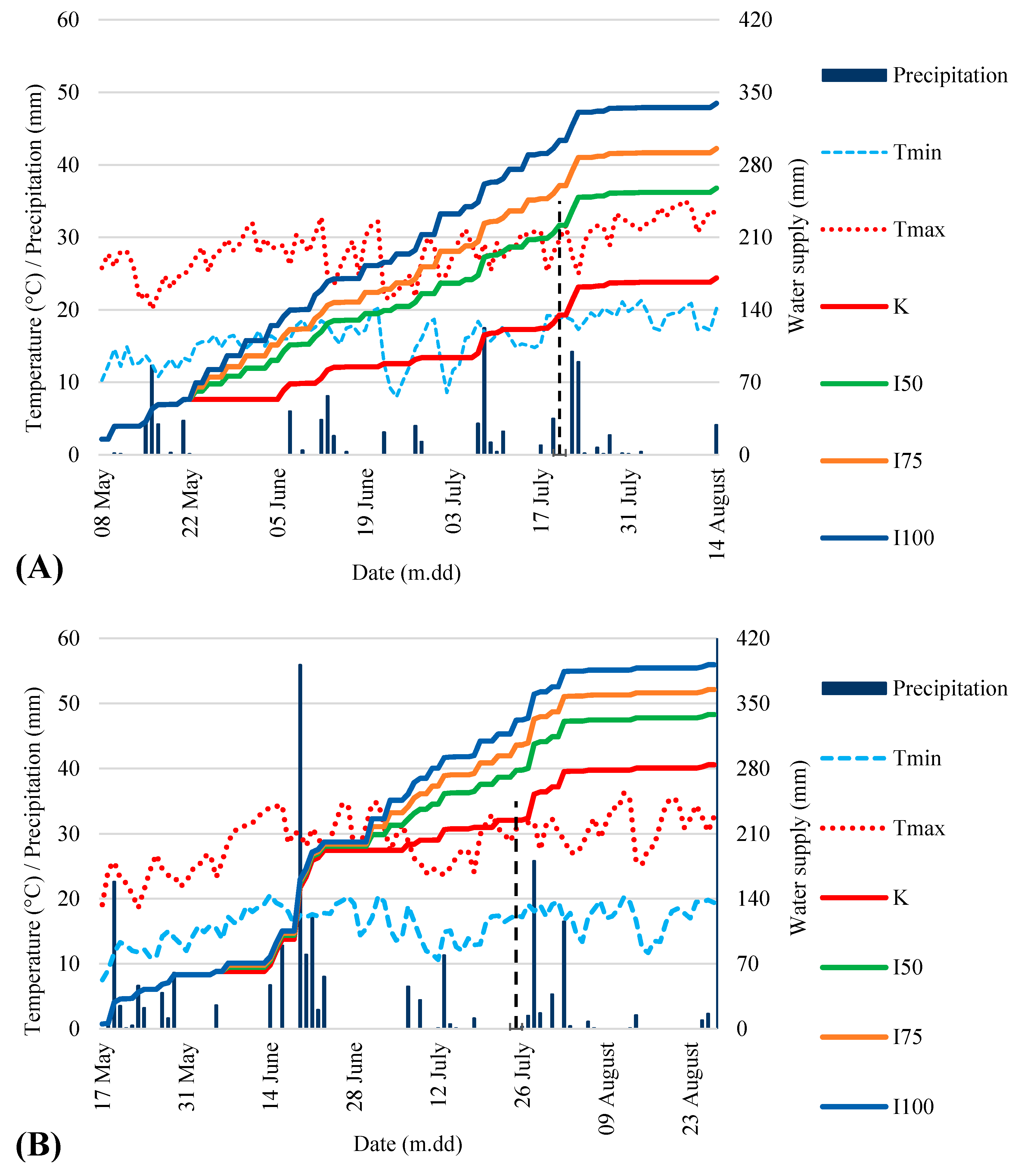
3.1. Meteorology, Irrigation

Climate conditions have a strong influence on the irrigation water needs and the stress levels of plants, thus we wanted to provide a detailed picture of the two seasons. The temperature was basically the same in both years regarding the mean temperatures of the whole growing season as well as of July. However, significant difference was registered in the precipitation of the whole season, which had doubled in 2019, compared to the previous year. In spite of this, the precipitation sum in July was basically the same in both years (Table 2).
A more detailed picture of the weather in July is shown (Figure 1). The temperature fluctuated more in 2019, causing a cooler period in the middle of the month. There were 16 days with some amount of rainfall, but only 3 of them were higher than 5 mm in 2018. This happened on 4 out of 12 days in 2019. Irrigation was ended 73 days after planting in 2018 and 69 days after planting in 2019.

3.2. Yields

Biomass production followed the same pattern in both years. Tomato reached much higher biomass yield in 2019, because the treatments received more water supply as the potential evapotranspiration was also higher. Season’s clear significant effect verifies this (Table 3). The same is true for total yields. However, marketable yields did not follow the same pattern. The highest marketable yield was reached in the I100 treatment in 2018 and 2019 as well, but the difference between I50 and I75 is not present in 2019. Explanation can be found in the green and non-marketable fruit yield. These show that green and non-marketable fruits together were higher in the I75 and I100 treatments in 2019 than in 2018. The ratio of green fruit yield was lower in the case of K and I50 and higher in the I75 and I100 treatments in 2019 (Table 4 and Table 5).
The crop’s potential evapotranspiration for the whole growing season calculated by AquaCrop is shown on Table 2. The difference between I100 water supply and ETc mostly comes from the period without irrigation before harvest. According to the findings of Kuşçu et al. [50], the best marketable yields (100.4 and 110.7 t ha−1) was reached always with the highest water supply rate; however, in their experiment the water restrictions were bound to different phenological stages and water restrictions were constant in our case in the deficit irrigated treatment. Highest marketable yields were found under the highest water supply in our case as well, but in 2019, the marketable yield of I50 is closer to I100 than the I75 treatment. As a meta-analysis study suggests, the rate of regulated deficit irrigation should be no less than 50% of water demand, because under this level, the water stress is too severe [51]. This is confirmed by our results in the case of marketable yield and only in 2018, since it reduced to 50.8%, but in 2019 it reduced only to 86.1%. However, it should be noted, that the water deficit was 82 mm in 2018 and only 54 mm in 2019 in the I50 treatment. According to Valcárcel et al. [52] irrigation with moderate water restriction (75% of crop ET) after fruit set does not cause yield reduction and mild restrictions (50% of crop ET) is recommended because of the increased functional quality of tomato production and considerable water savings. Though, the water restriction started from the beginning of fruit growing stage and it was not constant. Besides, they produced higher yields in the two years (118.18–157.88 t ha−1). In a study of evaluation of different tomato production scenarios, it was concluded that water saving practices that cause higher than mild water stress are not feasible under current climatic situation from a yield loss perspective [53], which is in agreement with our findings in the case of total yields. However, the use of different mulches can totally exclude the yield reduction effect of deficit irrigation [54], but the application of these mulches is problematic on large areas of open field farming.
The soluble solids yield is a very important factor in processing tomato production. Thus, the effect of water supply on it is widely researched and we also evaluated how the water supply affected SSC yield in our experiment. Water supply had a significant effect on SSC yields (p < 0.01) according to the two-year data. Differences appeared between the K and the I100 and I75 treatments. The most important result is that nor I50 neither I75 differed significantly from I100 treatment. This suggests that the same amount of soluble solids yield can be reached with deficit irrigation as well as with maximum water supply. However, only the upper quartile of I50 represents high enough SSC yields and 50% of the values are low, this means that I50 treatment is not reliable. I75 provided more safe soluble solids production along with I100.
Henceforth, the effect of water shortage stress on the tomato yields will be presented. Beforehand, the relationship between the water supply and the water stress was evaluated which is a linear relationship with R2 = 0.88 representing a strong connection (data not shown).

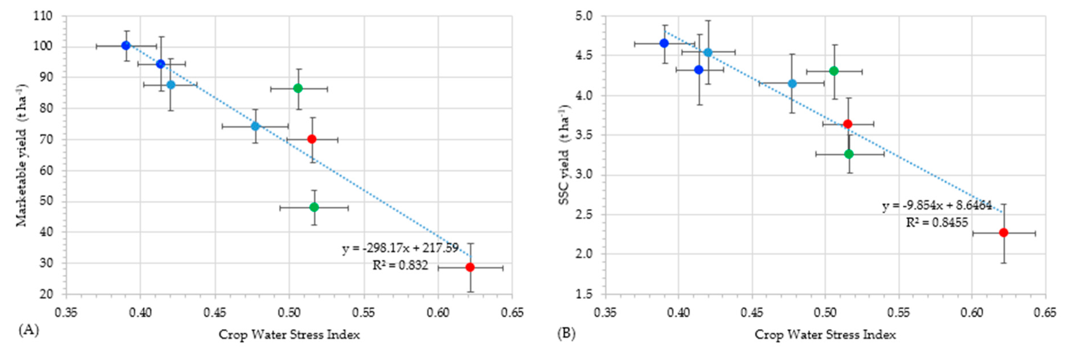
3.3. Effect of Irrigation

The effect of irrigation can be well illustrated on a PCA biplot (Figure 2). The different irrigation strategies are well differentiated by the ellipses enclosing the different groups. Eleven factors were used for the two principal components of the PCA. These two together explains 90.8% of the total variance of the data. Factors such as SSC-, biomass-, total, and marketable yield affected the first principal component and the two different carotenoids and their yields along with the stress values and SSC affected mostly the second principal component. The I100 group shows clear independence from the other two irrigated groups and from the control. The control slightly overlaps with the I50. The biggest overlap is between the two deficit irrigated groups according to the PCA. These overlaps are caused due to the results of 2019, where K, I50 and I75 are close to each other regarding different factors such as lycopene concentration, CWSI or marketable yield.

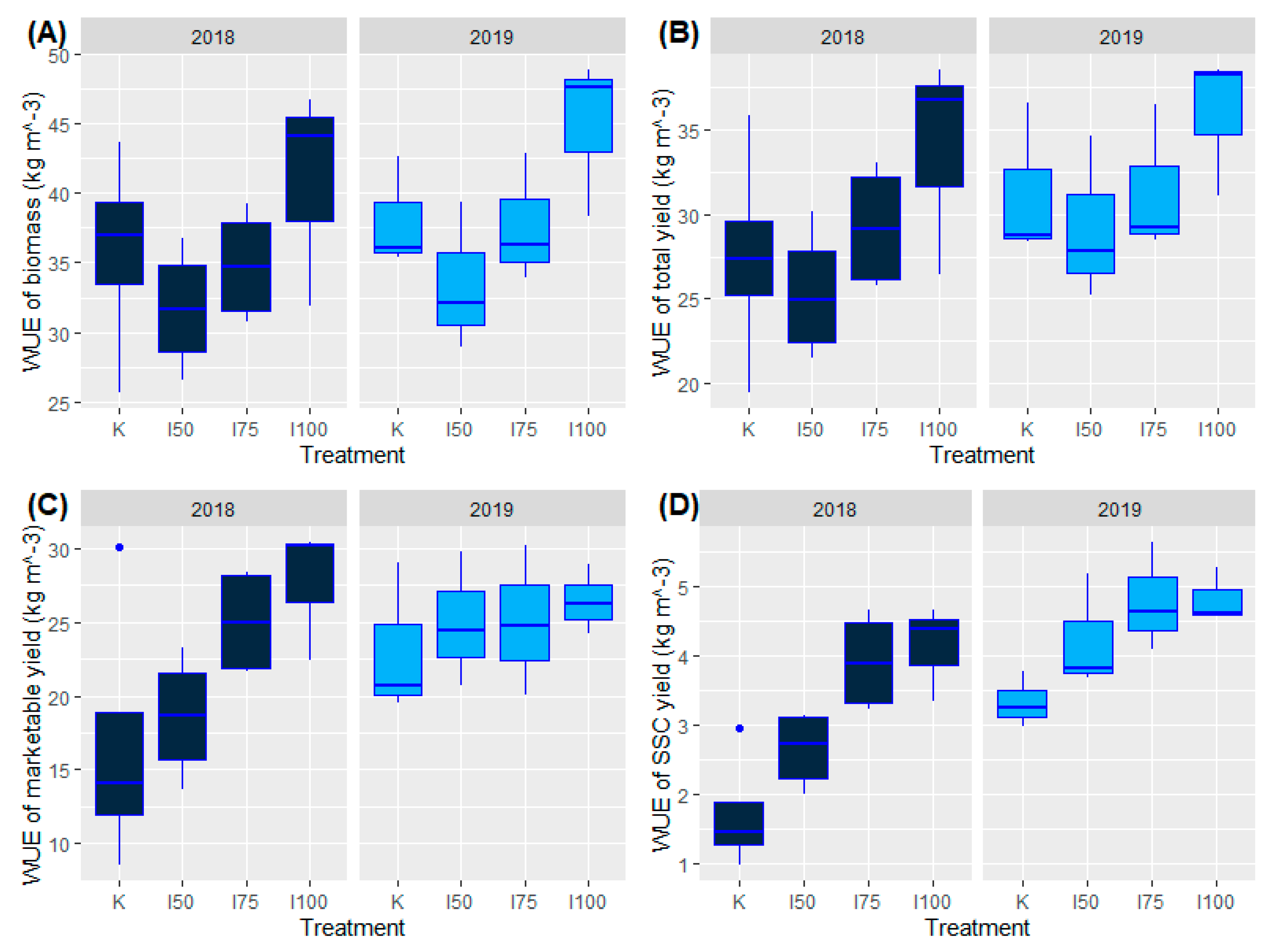
3.4. Effect of Water Supply on Water Use Efficiency

The effect of water supply levels on the water use efficiency, in the case of biomass and total yield shows the same pattern for both years where the highest means were produced in the I100 treatment and the lowest in the I50 (Figure 3). WUE of marketable yield reveal inconsistent results, since data show different patterns in the two years. The WUE of marketable yields shows step-like increase in 2018 from the lowest water supply to the highest. The highest mean was found in the I100 treatment, which also produced the highest yield in 2019, but the means of other treatments are very close to I100. One of the reasons for the confusing results is the big standard deviation in some cases, especially in the control of 2018. We could not find any significant difference between treatments evaluating the two years separately, but it is important to note, that the p-value was on the edge in several cases such as WUE for marketable yield in 2018. Though others found lower WUE values than was found by us, it clearly proved the enhanced WUE of deficit irrigation compared to full and unirrigated [55,56]. In our case higher WUE tend to be come with higher water supply levels, since I100 reached higher WUE in the case of biomass, marketable- and total yield. According to the results of Giuliani et al. [57] when applying partial root-zone drying, the 70% of ETc result in significantly better WUE regarding marketable yield than the treatment receiving 100% of ETc. However, they found the best WUE in the treatment irrigated only at transplanting and fertigation. Different deficit irrigations were investigated by another study [50], where WUE of marketable yield ranged 10.5–21.4 kg m−3. The highest WUE was found when irrigation was conducted throughout the growing season except the ripening stage, which agrees with our findings, because we also ended irrigation in the beginning of the ripening stage. No significant difference was found between treatments regarding WUE of SSC yield, however the same levels of WUE was reached in the I75 and I100 treatments, which is very good result with such an important factor of processing tomato as SSC yield.

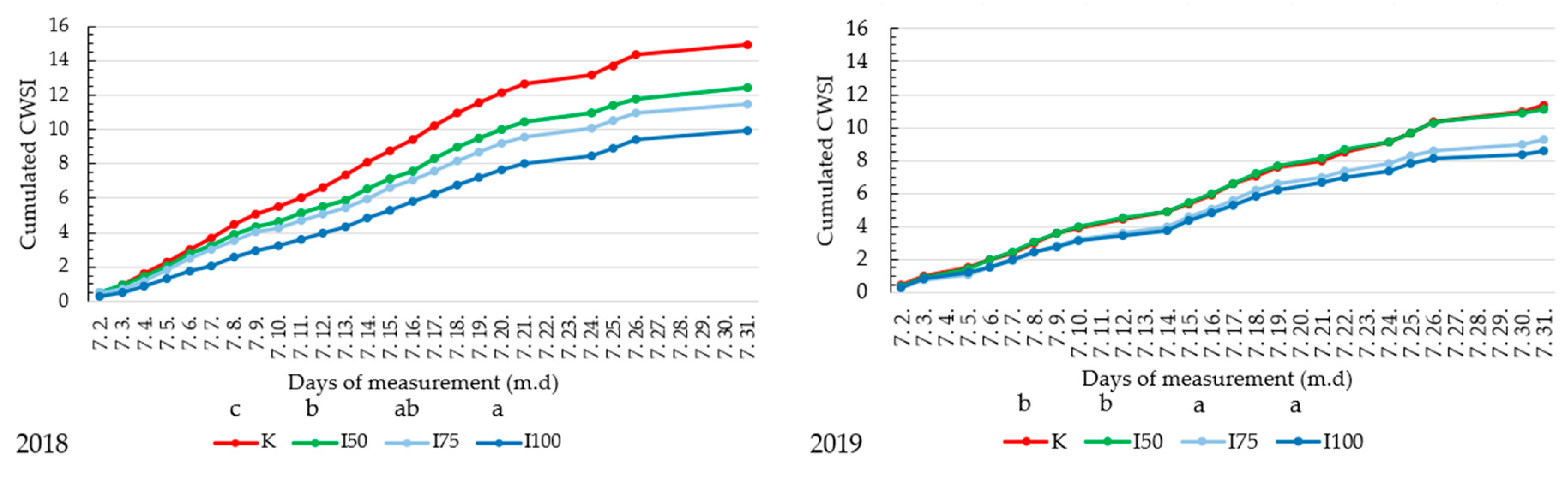
3.5. Effect of Stress Levels

The CWSI values in 2018 was statistically different in the case of K, I50, and I100. The values in the I75 treatment were similar to both of I100 and I50 treatments. The values were not well distinguished in 2019, where K and I50 were statistically the same and the I100 and I75 also. Thus, the K and I50 were exposed to the same stress level according to the ANOVA and post hoc test, and the other two treatments represented another stress level, lower than K and I50 (Figure 4). Giuliani et al. [57] found significantly different CWSI values for the treatments restoring 100% of ETc and 70% of ETc. The treatment irrigated only at transplanting and fertigation was different as well from the regularly irrigated treatments. In our case the difference was not clear between I75 and I100 in 2018, and the treatments were statistically the same in 2019.
In our case, the best option to assess the water shortage stress levels was to use the average of the measured CWSI values. The significant (p < 0.01) effect of water stress on biomass production was confirmed by a polynomial relationship giving an R2 of 0.87. Linear regression gives the best fit for total yields where R2 = 0.86 at p < 0.001 significance level. The regression line for the CWSI and marketable yield is linear. The points are only scattered in the center of the plot and the relationship is significant (R2 = 0.83, p = 0.002). This suggests that the best marketable yields comes with lower stress, and there is a breakpoint around 0.51 CWSI, above which marketable yields drop significantly (Figure 5A). Also linear, but weaker relationship was found between fruit yield and CWSI by others [58]. Total and marketable fruit yield appeared to be the highest at lower stress levels, we evaluated the formation of the green and non-marketable yields. According to the two-way ANOVA, the year had significant effect on green fruit yield, which seems to be clear, because in 2019 higher green fruit yields were produced (Table 3). Besides this, the interaction of year and treatment also showed significant effect. However, the stress levels had no effect of green yields, according to regression analysis.
The relationship between SSC yield and water stress levels are similar to the previous but it gives slightly better fit with the regression line. The relationship between the two factors is slightly better than the previous R2 = 0.85, at p = 0.001 significance level (Figure 5B). The two models are basically the same. When the stress is above 0.51 average CWSI, the SSC yield drops below 4 t ha−1.
Considering comprehensive tomato growth modelling results, other researchers suggested that the optimal water supply might be around 60–70% of crop evapotranspiration in the future, because of the predicted effects of climate change and heat stress identification will reduce irrigation water availability. The study emphasized the beneficial effects of moderate water stress during the ripening stage of tomato [59]. The increasement in dry yield induced by water deficit can be genotype dependent as well and not only the effect of water deficit [60].

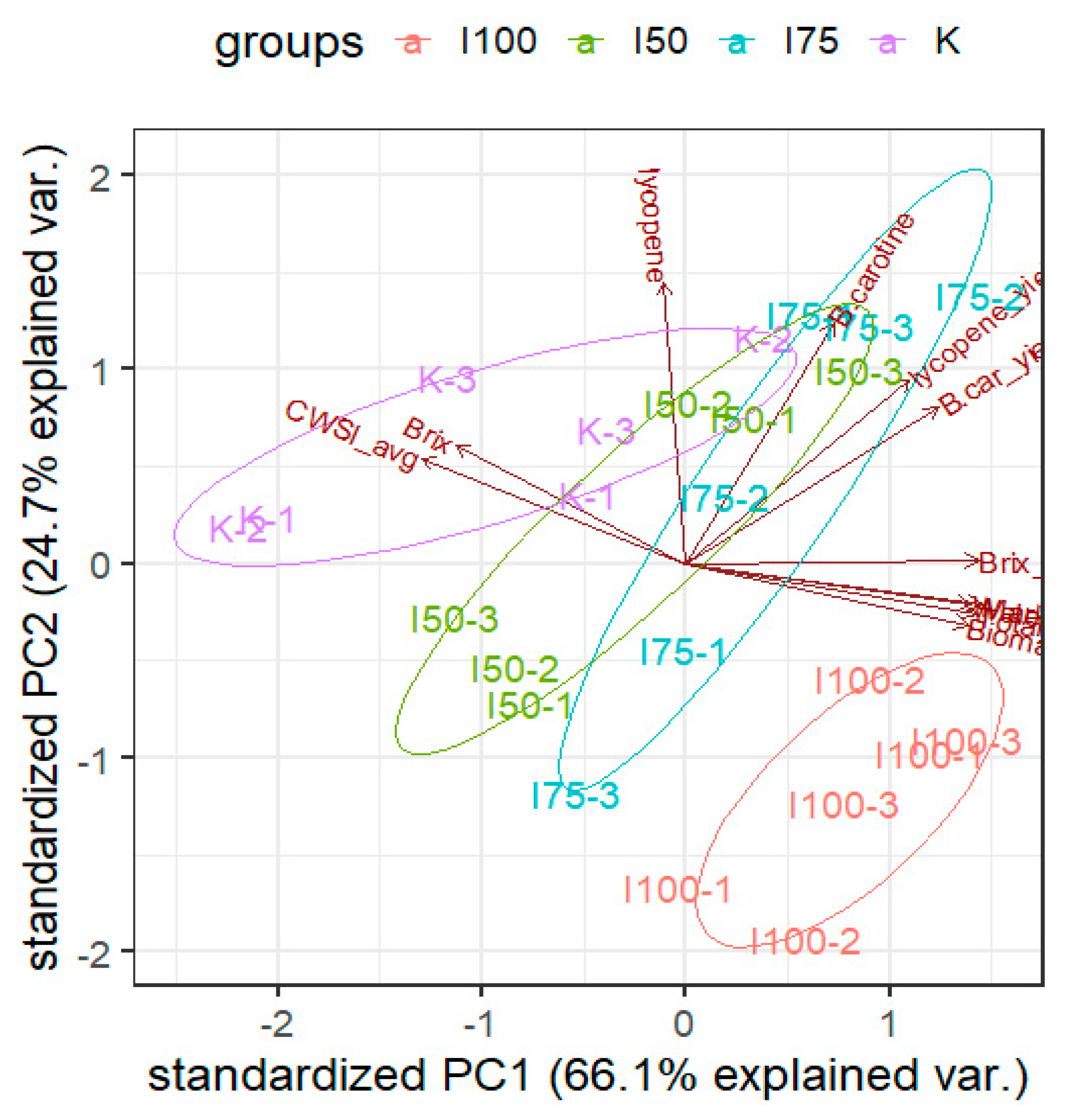
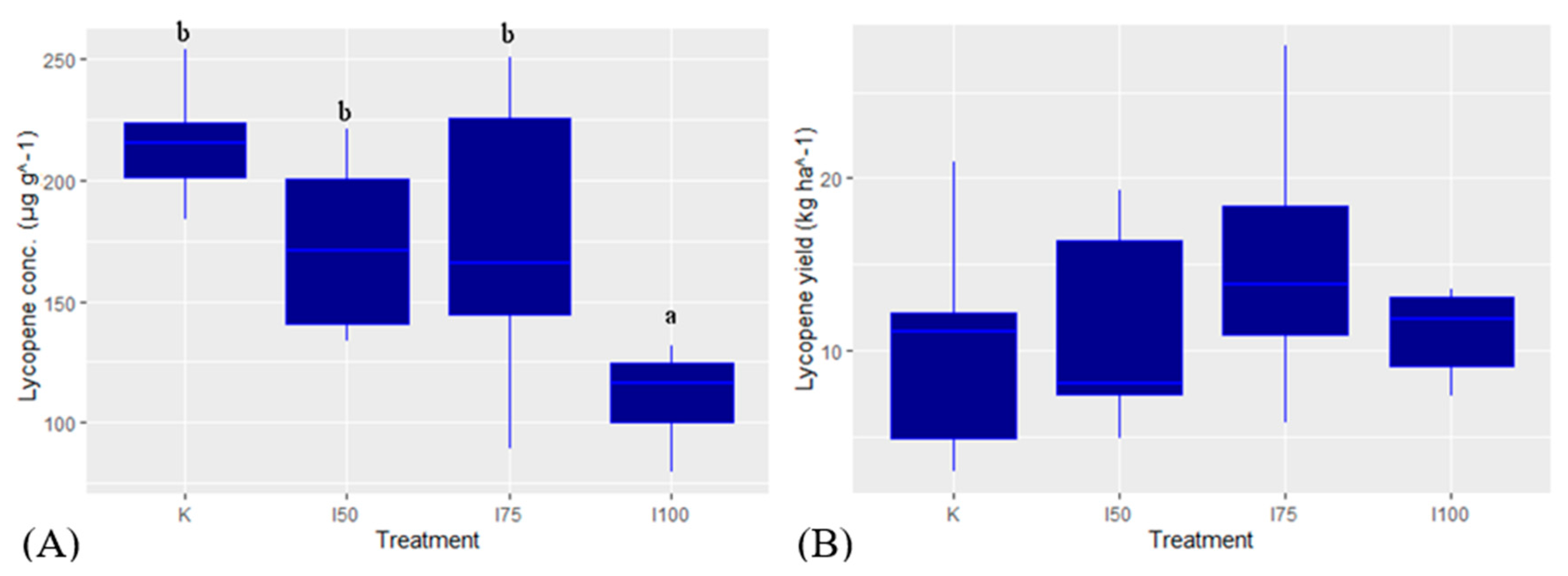
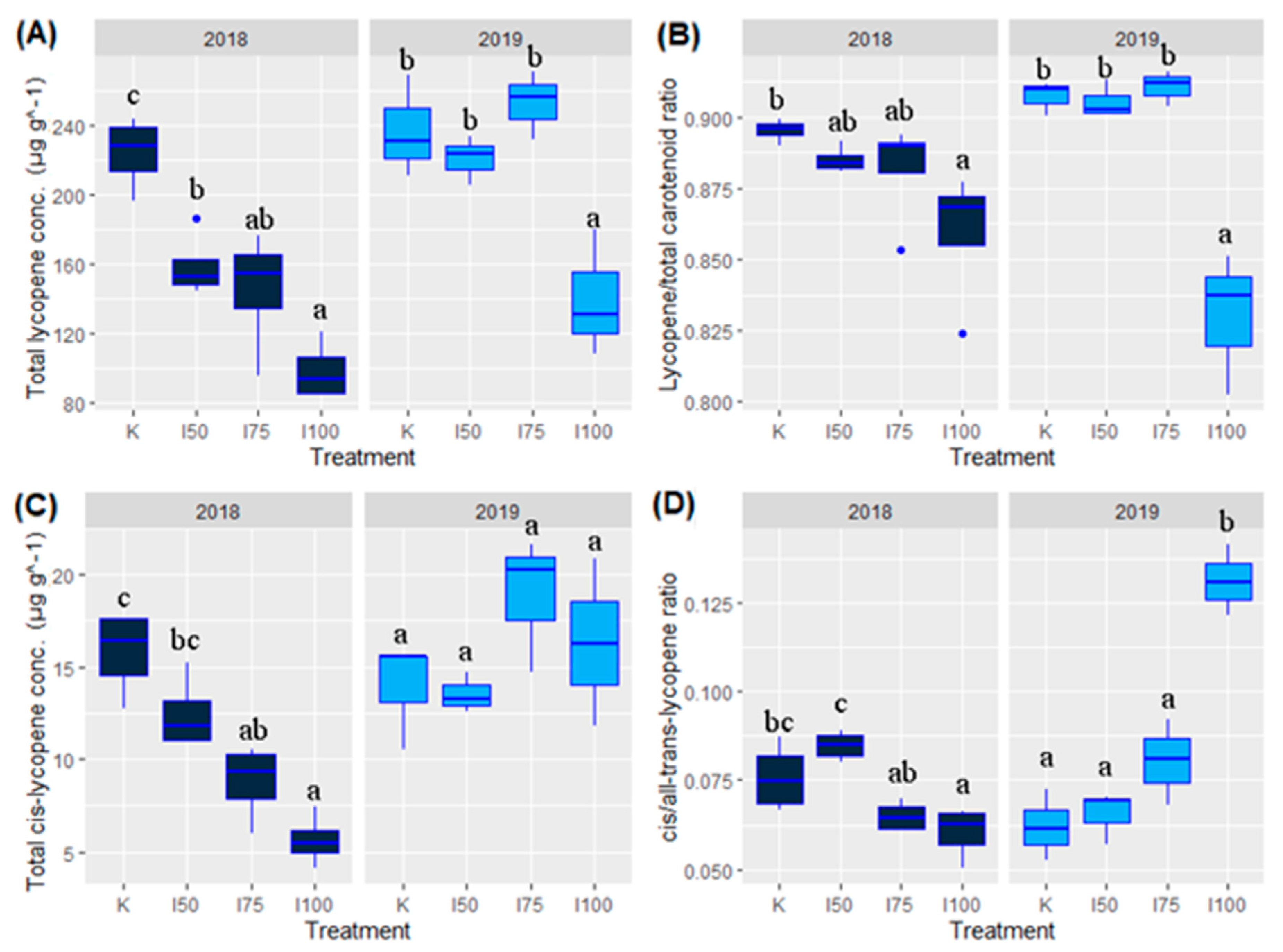
3.6. Effect of Water Supply and Season on Lycopene

A two-way ANOVA was also conducted to analyze the effect of water supply on the lycopene concentration in the fruits. The results revealed that both year and treatment and also their interaction had significant effect on tomato’s most important carotenoid (p < 0.01). When examined the means of the two-year values, we noticed that the water stress levels had a clear effect on carotenoid content of tomato. There is a significant difference between treatments as showed in Figure 6.
In both cultivation seasons, the highest concentration of lycopene was recorded in the control (K) treatment, while the lowest level was found in the I100 treatment that had the highest water supply (Figure 6). The two years differed in the effect of water supply on the lycopene content of the fruits. In 2019, the lycopene concentrations were very similar to that found in the K treatment, but this was not the case in 2018, when the concentrations of the deficit irrigated treatments were between the levels determined in the K and I100 treatments. In 2018, the lycopene concentration in the K treatment differed significantly from the content measured in the other treatments. In 2018, the I50 and I100 has differed significantly. The highest lycopene concentrations had been found in the rainfed treatment by other studies too [61,62]. Bogale et al. [55] found a significant effect of higher water supply on lycopene concentration, but according to their results the effect is most likely cultivar- dependent in tomato. It needs to be mentioned that the lack of statistical differences in some cases such as cis-lycopene concentration is due to very high standard deviation values obtained between the biological replications.
Despite the high marketable yields of tomato cultivated with I100 water supply, the low level of lycopene in the fruits makes it necessary to consume higher quantities to compensate the recommended daily intake of lycopene. In the I75 treatment lycopene yield was higher 10 kg ha−1, and the maximum yield of 27.67 kg ha−1 was reached in a replication of I75 treatment as well. The K and I50 treatments produced the same levels of lycopene yield. The highest lycopene yield has been produced in the rainfed treatment, but there was no significant difference between the deficit and full irrigation treatments as found by Le et al. in 2018 [62].
The total carotenoid and total lycopene concentrations followed the same pattern in both years and in all treatments also the ANOVA and the post hoc test revealed the same statistical differences in both cases (total carotenoid concentration data not shown). That is because lycopene is tomato’s most important carotenoid, which provides the highest proportion of the carotenoid composition. Significantly higher concentrations of total lycopene can be found in greenhouse grown red ripe tomato (>302 μg g−1) than the highest that we found in this experiment (233 μg g−1) [63]. In 2019, the fruits in the control and deficit irrigated treatments contained carotenoids in similar concentrations, but it was significantly less in the I100. In 2018, the K contained higher concentrations than all the irrigated treatments. The same is true for lycopene concentrations (Figure 7A), due to the diluting effect of irrigation in 2018 [64], but the concentration were basically the same in K, I50 and I75 in 2019. Student’s t-test was performed to see the differences between the two years in the carotenoid and lycopene concentration and the test verified that the concentrations in the two years were unlike (p < 0.01). Comparing the treatments using the two-year data indicates that only the I100 had less concentration than the other three in the case of total lycopene. The ratio of lycopene and total carotenoid concentrations shows the ratio of all trans lycopene in this case (Figure 7B). However, there was no difference between the two years; comparing the treatments we got almost the same result as in the comparison of total lycopene concentrations (from the two-year data).
The cis-lycopene concentration was the same in all treatments in 2019 according to the results of the post-hoc test (Figure 7C). The treatments with moderate and severe water stress reached higher concentrations of cis-isomers in 2018, than I75 and I100. Therefore, our findings do not consistently point in one direction in this case. No cis-isomers were found in fresh tomatoes in a previous study, which showed how the ratio of cis-isomers to all-trans is increasing due to different dehydration processes [65]. The evaluation of cis- and all trans-lycopene ratio gave confusing results. There was no significant difference between years or treatments when we evaluated the two-year data. The comparison of treatments in the two different years is not adequate to draw clear conclusions. The reason for that is, that in 2018 the I50 and control reached higher cis ratios, but in 2019 only the I100 was significantly higher than the others (Figure 7D). The explanation may be that in 2019, the K, I50, and I75 reached high lycopene concentrations and similar cis to all-trans ratios. However, the I100 presented the same level of cis-lycopene concentration as the other treatments, even if the total lycopene concentration was lower compared to K, I50, and I75 in 2019. On the other hand, slightly higher (around 0.15) cis to all-trans ratio found by others in fresh tomatoes compared to the highest ratio in our study (around 0.13) [66].

4. Conclusions

The highest yields were reached at the lowest water shortage stress levels. The I100 produced the best marketable yield in both years. From marketable and SSC yield perspective, the optimal water supply was provided in the I75 and I100 treatments. The WUE reached the same levels in the I100 and I75 treatments in the case of important production factors as marketable- and SSC yield. But, from lycopene concentration and -yield perspective the I75 proved to be better option, because of the significantly higher concentration regarding the summarized results in the two years, which could compensate the lower marketable yield, reaching the same or higher lycopene yields. High lycopene concentration results from low water supplies. Since lycopene concentrations are significantly lower in the I100, and K provides low yields, thus deficit irrigation is very beneficial, because the lycopene concentration in the fruit is good and it provides high lycopene yields as well, especially in the case of 75% of ETc water supply until the beginning of ripening stage. Nowadays, beside producing enough food, our other goal is to produce healthier, high quality food. In the case of tomato, higher lycopene concentration can serve this goal. However, I75 tend to be better than I100 only in one year regarding some evaluated factors, it reaches the same levels as I100 in the other year. This fact suggests, that I75 provides the same level of SSC and lycopene even if the raw material is less. The transportation of raw material from field to the processing factory can be more economic this way, and also water and energy savings can be reached. Our presented data indicates that the optimal water supply is between 300–370 mm for processing tomato under open field conditions and under the environmental and ecological conditions of south-east Hungary, which could be extended to the wider region of Central Europe. Moreover, water savings provided by I75 compared to the I100 can be significant on a large scale (27–43 mm), so we suggest the use of the 75% of ETc water supply until the beginning of ripening stage for processing tomato production under the examined conditions. According to our findings in the two different years, the cis and all-trans ratio or the cis-lycopene concentration was not clearly influenced by water supply levels, but important to note that we analyzed only two years, therefore, the data did not show consistent results.

Author Contributions

Conceptualization, L.H., G.P. and S.T.; methodology, Z.P., P.S. and H.G.D.; software, S.T.; validation, L.H. and Z.P.; formal analysis, Z.P.; investigation, S.T. and D.C.; resources; L.H. data curation, S.T.; writing—original draft preparation, S.T.; writing—review and editing, L.H., G.P., P.S. and Z.P.; visualization, S.T.; supervision, L.H. and Z.P.; funding acquisition, L.H., G.P., P.S. All authors have read and agreed to the published version of the manuscript.

Funding

The open field experiments were funded by GINOP 2.2.1-15-2016-00003. This paper and the research work was supported by the Higher Education Institutional Excellence Program (NKFIH-1159-6/2019) awarded by the Ministry for Innovation and Technology within the framework of water-related research of Szent István University and the EFOP-3.6.3-VEKOP-16-2017-00008 projects.

Acknowledgments

We would like to thank everyone who contributed to this article, especially to the field technical workers and the laboratory crew.

Conflicts of Interest

The authors declare no conflict of interest.

References

  1. Luo, T.; Young, R.; Reig, P. Aqueduct Projected Water Stress Country Rankings. In Technical Note; World Resources Institute: Washington, DC, USA, 2015. [Google Scholar]
  2. Helyes, L.; Gy, V.; Pék, Z.; Dimény, J. The simultaneous effect of variety, irrigation and weather on tomato yield. Acta Hortic. 1999, 487, 499–505. [Google Scholar] [CrossRef]
  3. Huang, J.; Wu, P.; Zhao, X. Effects of rainfall intensity, underlying surface and slope gradient on soil infiltration under simulated rainfall experiments. Catena 2013, 104, 93–102. [Google Scholar] [CrossRef]
  4. Nemeskéri, E.; Neményi, A.; Bocs, A.; Pék, Z.; Helyes, L. Physiological factors and their relationship with the productivity of processing tomato under different water supplies. Water (Switzerland) 2019, 11, 586. [Google Scholar] [CrossRef] [Green Version]
  5. Helyes, L.; Bocs, A.; Lugasi, A.; Pék, Z. Tomato antioxidants and yield as affected by different water supply. Acta Hortic. 2012, 936, 213–218. [Google Scholar] [CrossRef]
  6. Pék, Z.; Szuvandzsiev, P.; Neményi, A.; Helyes, L. Effect of season and irrigation on yield parameters and soluble solids content of processing cherry tomato. Acta Hortic. 2015, 1081, 197–202. [Google Scholar] [CrossRef]
  7. Unlu, N.Z.; Bohn, T.; Francis, D.M.; Nagaraja, H.N.; Clinton, S.K.; Schwartz, S.J. Lycopene from heat-induced cis-isomer-rich tomato sauce is more bioavailable than from all-trans-rich tomato sauce in human subjects. Br. J. Nutr. 2007, 98, 140–146. [Google Scholar] [CrossRef] [Green Version]
  8. Kelkel, M.; Schumacher, M.; Dicato, M.; Diederich, M. Antioxidant and anti-proliferative properties of lycopene. Free Radic. Res. 2011, 45, 925–940. [Google Scholar] [CrossRef]
  9. Caseiro, M.; Ascenso, A.; Costa, A.; Creagh-Flynn, J.; Johnson, M.; Simões, S. Lycopene in human health. LWT Food Sci. Technol. 2020, 127, 109323. [Google Scholar] [CrossRef]
  10. Helyes, L.; Pék, Z.; Lugasi, A. Function of the variety technological traits and growing conditions on fruit components of tomato (Lycopersicon lycopersicum (L) Karsten). Acta Aliment. 2008, 37, 427–436. [Google Scholar] [CrossRef]
  11. Ilahy, R.; Siddiqui, M.W.; Tlili, I.; Montefusco, A.; Piro, G.; Hdider, C.; Lenucci, M.S. When Color Really Matters: Horticultural Performance and Functional Quality of High-Lycopene Tomatoes. CRC. Crit. Rev. Plant Sci. 2018, 37, 15–53. [Google Scholar] [CrossRef]
  12. Ilahy, R.; Tlili, I.; Siddiqui, M.W.; Hdider, C.; Lenucci, M.S. Inside and beyond color: Comparative overview of functional quality of tomato and watermelon fruits. Front. Plant Sci. 2019, 10, 1–26. [Google Scholar] [CrossRef] [PubMed] [Green Version]
  13. Martí, R.; Valcárcel, M.; Leiva-Brondo, M.; Lahoz, I.; Campillo, C.; Roselló, S.; Cebolla-Cornejo, J. Influence of controlled deficit irrigation on tomato functional value. Food Chem. 2018, 252, 250–257. [Google Scholar] [CrossRef] [PubMed]
  14. Lahoz, I.; Pérez-de-Castro, A.; Valcárcel, M.; Macua, J.I.; Beltrán, J.; Roselló, S.; Cebolla-Cornejo, J. Effect of water deficit on the agronomical performance and quality of processing tomato. Sci. Hortic. (Amsterdam) 2016, 200, 55–65. [Google Scholar] [CrossRef] [Green Version]
  15. Helyes, L.; Dimény, J.; Bocs, A.; Schober, G.; Pék, Z. The effect of water and potassium supplement on yield and lycopene content of processing tomato. Acta Hortic. 2009, 823, 103–108. [Google Scholar] [CrossRef]
  16. Kuscu, H.; Turhan, A.; Ozmen, N.; Aydinol, P.; Demir, A.O. Optimizing levels of water and nitrogen applied through drip irrigation for yield, quality, and water productivity of processing tomato (Lycopersicon esculentum Mill.). Hortic. Environ. Biotechnol. 2014, 55, 103–114. [Google Scholar] [CrossRef]
  17. Favati, F.; Lovelli, S.; Galgano, F.; Miccolis, V.; Di Tommaso, T.; Candido, V. Processing tomato quality as affected by irrigation scheduling. Sci. Hortic. (Amsterdam) 2009, 122, 562–571. [Google Scholar] [CrossRef]
  18. Helyes, L.; Szuvandzsiev, P.; Neményi, A.; Pék, Z.; Lugasi, A. Different water supply and stomatal conductance correlates with yield quantity and quality parameters. Acta Hortic. 2013, 971, 119–126. [Google Scholar] [CrossRef]
  19. Campillo, C.; Carrasco, J.; Gordillo, J.L.; Cordoba, A.; Macua, J.I. Use of satellite images to differentiate productivity zones in commercial processing tomato farms. Acta Hortic. 2019, 1233, 97–104. [Google Scholar] [CrossRef]
  20. Bőcs, A.; Pék, Z.; Helyes, L.; Neményi, A.; Komjáthy, L. Effect of water supply on canopy temperature and yield of processing tomato. Cereal Res. Commun. 2009, 37, 113–116. [Google Scholar] [CrossRef]
  21. Fuchs, M. Infrared Measurement of Canopy Temperature and Detection of Plant Water Stress. Theor. Appl. Climatol. 1990, 42, 253–261. [Google Scholar] [CrossRef]
  22. Nemeskéri, E.; Molnár, K.; Pék, Z.; Helyes, L. Effect of water supply on the water use-related physiological traits and yield of snap beans in dry seasons. Irrig. Sci. 2018, 36, 143–158. [Google Scholar] [CrossRef]
  23. Nemeskéri, E.; Molnár, K.; Vígh, R.; Nagy, J.; Dobos, A. Relationships between stomatal behaviour, spectral traits and water use and productivity of green peas (Pisum sativum L.) in dry seasons. Acta Physiol. Plant. 2015, 37, 34. [Google Scholar] [CrossRef]
  24. Christmann, A.; Hoffmann, T.; Teplova, I.; Grill, E.; Mu, A. Generation of Active Pools of Abscisic Acid Revealed by In Vivo Imaging of Water-Stressed Arabidopsis 1. Plant Physiol. 2005, 137, 209–219. [Google Scholar] [CrossRef] [PubMed] [Green Version]
  25. Helyes, L.; Pék, Z.; McMichael, B. Relationship between the stress degree day index and biomass production and the effect and timing of irrigation in snap bean (Phaseolus vulgaris var. nanus) stands: Results of a long term expeiments. Acta Bot. Hung. 2006, 48, 311–321. [Google Scholar] [CrossRef]
  26. Nemeskéri, E.; Helyes, L. Physiological Responses of Selected Vegetable Crop Species to Water Stress. Agronomy 2019, 9, 447. [Google Scholar] [CrossRef] [Green Version]
  27. Jackson, R.D.; Idso, S.B.; Reginato, R.J.; Pinter, J.P.J. Canopy temperature as a crop water stress indicator. Water Resour. Res. 1981, 17, 1133–1138. [Google Scholar] [CrossRef]
  28. Jackson, R.D.; Kustas, W.P.; Choudhury, B.J. A reexamination of the crop water stress index. Irrig. Sci. 1988, 9, 309–317. [Google Scholar] [CrossRef]
  29. O’Shaughnessy, S.A.; Evett, S.R.; Colaizzi, P.D.; Howell, T.A. A crop water stress index and time threshold for automatic irrigation scheduling of grain sorghum. Agric. Water Manag. 2012, 107, 122–132. [Google Scholar] [CrossRef] [Green Version]
  30. Takács, S.; Pék, Z.; Bíró, T.; Helyes, L. Heat stress detection in tomato under different irrigation treatments. Acta Hortic. 2019, 1233, 47–52. [Google Scholar] [CrossRef]
  31. Khapte, P.S.; Kumar, P.; Burman, U.; Kumar, P. Deficit irrigation in tomato: Agronomical and physio-biochemical implications. Sci. Hortic. (Amsterdam) 2019, 248, 256–264. [Google Scholar] [CrossRef]
  32. El-Marsafawy, S.M.; Swelam, A.; Ghanem, A. Evolution of crop water productivity in the Nile Delta over three decades (1985-2015). Water (Switzerland) 2018, 10, 1168. [Google Scholar] [CrossRef] [Green Version]
  33. Hungarian Meteorological Service Climate of Hungary—General Characteristics. Available online: https://www.met.hu/en/eghajlat/magyarorszag_eghajlata/altalanos_eghajlati_jellemzes/altalanos_leiras/ (accessed on 10 June 2020).
  34. Nichols, M.A. Towards 10 t/ha Brix. Acta Hortic. 2006, 724, 217–223. [Google Scholar] [CrossRef]
  35. Van Halsema, G.E.; Vincent, L. Efficiency and productivity terms for water management: A matter of contextual relativism versus general absolutism. Agric. Water Manag. 2012, 108, 9–15. [Google Scholar] [CrossRef]
  36. Takács, S.; Bíró, T.; Helyes, L.; Pék, Z. Variable rate precision irrigation technology for deficit irrigation of processing tomato. Irrig. Drain. 2019, 68, 234–244. [Google Scholar] [CrossRef]
  37. Battilani, A.; Prieto, M.H.; Argerich, C.; Campillo, C.; Cantore, V. Tomato. In Fao Irrigation and Drainage Paper 66—Crop Yield Response To Water; Steduto, P., Hsiao, T.C., Fereres, E., Raes, D., Eds.; Food and Agriculture Organization of the United Nations: Rome, Italy, 2012; pp. 192–201. ISBN 9789251072745. [Google Scholar]
  38. Allen, R.G.; Pereira, L.S.; Raes, D.; Smith, M. Crop evapotranspiration—Guidelines for computing crop water requirements. In FAO Irrigation and Drainage Paper 56; FAO: Rome, Italy, 1998; p. D05109. [Google Scholar]
  39. Raes, D. AquaCrop Training Handbooks Book I Understanding AquaCrop; Food and Agriculture Organization of the United Nations: Rome, Italy, 2017; 50p, ISBN 978-92-5-109390-0. [Google Scholar]
  40. Steduto, P.; Hsiao, T.C.; Fereres, E.; Raes, D. Crop Yield Response to Water; Food and Agriculture Organization of the United Nations: Rome, Italy, 2012; 501p. [Google Scholar]
  41. Macua, J.I.; Lahoz, I.; Arzoz, A.; Garnica, J. The influence of irrigation cut-off time on the yield and quality of processing tomatoes. Acta Hortic. 2003, 613, 151–153. [Google Scholar] [CrossRef]
  42. Jones, H.G. Use of infrared thermometry for estimation of stomatal conductance as a possible aid to irrigation scheduling. Agric. For. Meteorol. 1999, 95, 139–149. [Google Scholar] [CrossRef]
  43. Costa, J.M.; Grant, O.M.; Chaves, M.M. Thermography to explore plant-environment interactions. J. Exp. Bot. 2013, 64, 3937–3949. [Google Scholar] [CrossRef]
  44. Maes, W.H.; Steppe, K. Estimating evapotranspiration and drought stress methylation and chromatin patterning with ground-based thermal remote sensing in agriculture: A review. J. Exp. Bot. 2012, 63, 4671–4712. [Google Scholar] [CrossRef] [Green Version]
  45. Grant, O.M.; Tronina, Ł.; Jones, H.G.; Chaves, M.M. Exploring thermal imaging variables for the detection of stress responses in grapevine under different irrigation regimes. J. Exp. Bot. 2007, 58, 815–825. [Google Scholar] [CrossRef]
  46. Daood, H.G.; Bencze, G.; Palotás, G.; Pék, Z.; Sidikov, A.; Helyes, L. HPLC analysis of carotenoids from tomatoes using cross-linked C18 column and MS detection. J. Chromatogr. Sci. 2014, 52, 985–991. [Google Scholar] [CrossRef] [Green Version]
  47. Chambers, J.M. Linear Models. In Statistical Models in S; Chambers, J.M., Hastie, T.J., Eds.; Wadsworth & Brooks/Cole: New York, NY, USA, 1992; pp. 95–144. [Google Scholar]
  48. Chambers, J.M.; Freeny, A.; Heiberger, R.M. Analysis of Variance; Designed Experiments. In Statistical Models in S; Chambers, J.M., Hastie, T.J., Eds.; Wadsworth & Brooks/Cole: New York, NY, USA, 1992; pp. 145–194. [Google Scholar]
  49. Mardia, K.V.; Kent, J.T.; Bibby, J.M. Multivariate Analysis; Academic Press: Cambridge, MA, USA, 1979; 518p. [Google Scholar]
  50. Kuşçu, H.; Turhan, A.; Demir, A.O.; Kuşçu, H.; Turhan, A.; Demir, A.O. The response of processing tomato to deficit irrigation at various phenological stages in a sub-humid environment. Agric. Water Manag. 2014, 133, 92–103. [Google Scholar] [CrossRef]
  51. Lu, J.; Shao, G.; Cui, J.; Wang, X.; Keabetswe, L. Yield, fruit quality and water use efficiency of tomato for processing under regulated deficit irrigation: A meta-analysis. Agric. Water Manag. 2019, 222, 301–312. [Google Scholar] [CrossRef]
  52. Valcárcel, M.; Lahoz, I.; Campillo, C.; Martí, R.; Leiva-Brondo, M.; Roselló, S.; Cebolla-Cornejo, J. Controlled deficit irrigation as a water-saving strategy for processing tomato. Sci. Hortic. (Amsterdam) 2020, 261, 108972. [Google Scholar] [CrossRef]
  53. Saadi, S.; Todorovic, M.; Tanasijevic, L.; Pereira, L.S.; Pizzigalli, C.; Lionello, P. Climate change and Mediterranean agriculture: Impacts on winter wheat and tomato crop evapotranspiration, irrigation requirements and yield. Agric. Water Manag. 2015, 147, 103–115. [Google Scholar] [CrossRef]
  54. Biswas, S.K.; Akanda, A.R.; Rahman, M.S.; Hossain, M.A. Effect of drip irrigation and mulching on yield, water-use efficiency and economics of tomato. Plant Soil Environ. 2015, 61, 97–102. [Google Scholar] [CrossRef] [Green Version]
  55. Bogale, A.; Nagle, M.; Latif, S.; Aguila, M.; Müller, J. Regulated deficit irrigation and partial root-zone drying irrigation impact bioactive compounds and antioxidant activity in two select tomato cultivars. Sci. Hortic. (Amsterdam) 2016, 213, 115–124. [Google Scholar] [CrossRef]
  56. Patanè, C.; Tringali, S.; Sortino, O. Effects of deficit irrigation on biomass, yield, water productivity and fruit quality of processing tomato under semi-arid Mediterranean climate conditions. Sci. Hortic. (Amsterdam) 2011, 129, 590–596. [Google Scholar] [CrossRef]
  57. Giuliani, M.M.; Nardella, E.; Gagliardi, A.; Gatta, G. Deficit irrigation and partial root-zone drying techniques in processing tomato cultivated under Mediterranean climate conditions. Sustainability 2017, 9, 2197. [Google Scholar] [CrossRef] [Green Version]
  58. Silva, C.J.D.; Silva, C.A.D.; Freitas, C.A.D.; Golynski, A.; da Silva, L.F.; Frizzone, J.A. Tomato water stress index as a function of irrigation depths. Rev. Bras. Eng. Agric. Ambient. 2018, 22, 95–100. [Google Scholar] [CrossRef] [Green Version]
  59. Giuliani, M.M.; Gatta, G.; Cappelli, G.; Gagliardi, A.; Donatelli, M.; Fanchini, D.; De Nart, D.; Mongiano, G.; Bregaglio, S. Identifying the most promising agronomic adaptation strategies for the tomato growing systems in Southern Italy via simulation modeling. Eur. J. Agron. 2019, 111, 125937. [Google Scholar] [CrossRef]
  60. Arbex de Castro Vilas Boas, A.; Page, D.; Giovinazzo, R.; Bertin, N.; Fanciullino, A.-L. Combined effects of irrigation regime, genotype, and harvest stage determine tomato fruit quality and aptitude for processing into puree. Front. Plant Sci. 2017, 8, 1725. [Google Scholar] [CrossRef] [PubMed]
  61. Helyes, L.; Lugasi, A.; Pék, Z. Effect of irrigation on processing tomato yield and antioxidant components. Turkish, J. Agric. For. 2012, 36, 702–709. [Google Scholar] [CrossRef]
  62. Le, T.A.; Pék, Z.; Takács, S.; Neményi, A.; Daood, H.G.; Helyes, L. The Effect of Plant Growth Promoting Rhizobacteria on the Water-yield Relationship and Carotenoid Production of Processing Tomatoes Zolt a. HortScience 2018, 53, 816–822. [Google Scholar] [CrossRef] [Green Version]
  63. Jarquín-Enríquez, L.; Mercado-Silva, E.M.; Maldonado, J.L.; Lopez-Baltazar, J. Lycopene content and color index of tomatoes are affected by the greenhouse cover. Sci. Hortic. (Amsterdam) 2013, 155, 43–48. [Google Scholar] [CrossRef]
  64. Helyes, L.; Le, T.A.; Bakr, J.A.; Pék, Z. The simultaneous effect of water stress and biofertilizer on physiology and quality of processing tomato. Acta Hortic. 2019, 53–60. [Google Scholar] [CrossRef]
  65. Shi, J.; Le Maguer, M.; Kakuda, Y.; Liptay, A.; Niekamp, F. Lycopene degradation and isomerization in tomato dehydration. Food Res. Int. 1999, 32, 15–21. [Google Scholar] [CrossRef]
  66. Stinco, C.M.; Rodríguez-Pulido, F.J.; Escudero-Gilete, M.L.; Gordillo, B.; Vicario, I.M.; Meléndez-Martínez, A.J. Lycopene isomers in fresh and processed tomato products: Correlations with instrumental color measurements by digital image analysis and spectroradiometry. Food Res. Int. 2013, 50, 111–120. [Google Scholar] [CrossRef]
Figure 1. Trend of maximum (Tmax) and minimum (Tmin) temperature, precipitation, and water supply for the four irrigation treatments in 2018 (A) and 2019 (B). Vertical dash line represents the date of last irrigation event.
Water 12 02165 g001
Figure 2. Biplot made from the results of the PCA (n = 3). The different water supply groups are shown with different colors. The different water supply levels are labeled on the plot in mm. The colored ellipses’ enclosing the water supply groups. Arrows show how the factors affect the principal components.
Water 12 02165 g002
Figure 3. The effect of different water supply treatments in both years on the water use efficiency, calculated for full biomass (A), the total yield (B), the marketable yield (C), and the soluble solids content (SSC) yield (D). No significant difference was found between treatments.
Water 12 02165 g003
Figure 4. Trend of cumulated crop water stress index (CWSI) in the two years. Different letters above treatments in the legend represent statistical differences as a result of Tukey post hoc test (p < 0.01).
Water 12 02165 g004
Figure 5. The relationship between the water stress values and marketable yield (R2 = 0.83) (A) and SSC yield (R2 = 0.85) (B). The vertical and horizontal bars represent the standard error.
Water 12 02165 g005
Figure 6. Effect of different water supplies on lycopene concentration (A) and yield (B) in tomato fruits. The values represent the average of two years. The values having the same letter above the boxes are statistically not significant (p > 0.05). No significant difference was found in the case of lycopene yield (B).
Water 12 02165 g006
Figure 7. Average of total lycopene (A) and cis-lycopene (C) content and lycopene/total carotenoid-(B) and cis-/all trans (D) lycopene ratio, under different water supply in two years. The different letters above the boxes indicate statistical differences between treatments inside one year (p < 0.05).
Water 12 02165 g007
Table 1. Date of planting and harvest and the fertilization in the two experimental years.
YearDate of PlantingDate of HarvestGrowing DaysN (kg ha−1)P (kg ha−1)K (kg ha−1)
20188 May14 August9813769174
201917 May27 August102138117183
Table 2. Major meteorological data for growing season also focusing on the period of the leaf surface temperature measurements (July).
Meteorological Data20182019
Mean temperature for growing season (°C)22.322.5
Mean temperature of July (°C)2322.4
Total precipitation for whole season (mm)126.9256.5
Total precipitation of July (mm)64.860.5
Mean relative humidity for whole season (%)6970.8
Mean relative humidity of July (%)69.167.3
Crop evapotranspiration for growing season (mm)445.5454.8
Crop evapotranspiration for irrigated period (mm)328.8321.3
Table 3. Two-way ANOVAs regarding tomato production variables.
VariableEffect of YearEffect of TreatmentEffect of Interaction
Biomass<0.001 ***<0.001 ***0.841
Total yield<0.001 ***<0.001 ***0.744
Marketable yield<0.001 ***<0.001 ***0.225
Green yield0.002 **0.3860.002 **
Non-marketable yield0.8030.039 *0.8
Stars represent different p-value thresholds: *** < 0.001, ** < 0.01, * < 0.05.
Table 4. Tomato production data for the two experimental years (Means ± Standard errors). “Water” column includes the summarized rainfall and irrigation water in the growing season in the treatments.
YearTreatmentWater
(mm)
Biomass
(t ha−1)
Total Fruit Yield
(t ha−1)
Marketable Fruit Yield
(t ha−1)
Green Fruit Yield
(t ha−1)
Non-Marketable Fruit Yield
(t ha−1)
SSC Yield
(t ha−1)
2018K17161.2 ± 6.3 a46.9 ± 5.6 a28.5 ± 7.8 a9 ± 1 b,c9.4 ± 4.2 a1.7 ± 0.4 a
I5025881.7 ± 5.8 a,b65.4 ± 5 a,b47.9 ± 5.5 a,b10.9 ± 1.5 c6.6 ± 2.2 a2.6 ± 0.3 a,b
I75297103.3 ± 6 b,c86.8 ± 5.4 b,c74.2 ± 5.4 b,c4.3 ± 0.3 a8.2 ± 0.8 a3.9 ± 0.4 b
I100340139.3 ± 15.2 c115.4 ± 12.5 c94.3 ± 8.7 c4.3 ± 1.1 a,b16.7 ± 3.3 a4.1 ± 0.4 b
2019K284110.5 ± 5.1 a91.4 ± 5.9 a69.9 ± 7.3 a12.2 ± 2 a9.0 ± 0.9 a3.6 ± 0.3 a
I50338118.9 ± 9.1 a103 ± 7.7 a86.3 ± 6.4 a6.4 ± 2 a10.0 ± 1 a4.3 ± 0.3 a
I75365136.4 ± 7 a,b114.8 ± 6.5 a,b87.6 ± 8.4 a13.1 ± 5.9 a13.7 ± 7.2 a4.5 ± 0.4 a
I100392170.7 ± 11.9 b136.9 ± 8.8 b100.2 ± 5.7 a22.1 ± 2.3 a14.1 ± 2.4 a4.6 ± 0.3 a
Different letters indicate statistically significant differences at p < 0.05 level regarding the different years.
Table 5. The ratio of marketable, green, and non-marketable fruit yield.
YearTreatmentRatio of Marketable Yield (%)Ratio of Green Yield (%)Ratio of Non-Marketable Yield (%)Fruits Per Plant (pcs)
2018K60.819.120.164.6 a
I5073.316.71065.4 a
I7585.659.458.4 a
I10081.73.814.572.1 a
2019K76.513.51069.5 a
I5083.86.39.876.4 a
I7576.311.612.1103.9 a,b
I10073.216.410.4119.9 b
Different letters indicate statistically significant differences at p < 0.05 level regarding the different years.

