Seasonal and Diurnal Variation of Air/Water Exchange of Gaseous Mercury in a Southern Reservoir Lake (Cane Creek Lake, Tennessee, USA)

Abstract

A year-long field study of mercury (Hg) air/water exchange was conducted at a southern reservoir lake, Cane Creek Lake (Cookeville, TN, USA). The Hg air/water exchange fluxes and meteorological data including solar radiation (global solar radiation, R_g and ultraviolent radiation, UVA), water and air temperatures, relative humidity, and wind speed were collected to study the daily and seasonal trends of the Hg air/water exchange at the lake in relation to solar radiation and wind speed. The Hg exchange fluxes generally exhibited diurnal patterns with a rise in the morning, a peak around noontime, and a fall in the afternoon through the evening, closely following the change of solar radiation. There were cases that deviated from this general daily trend. The Hg emission fluxes were all below 3 ng m⁻² h⁻¹ with the daily mean fluxes < 2 ng m⁻² h⁻¹. The fluxes in the summer (mean: 1.2 ng m⁻² h⁻¹) were higher than in the fall (mean: 0.6 ng m⁻² h⁻¹) and winter (mean: 0.7 ng m⁻² h⁻¹). The daily and seasonal trends of the Hg air/water exchange fluxes are similar to the trends of the changes of the dissolved gaseous mercury (DGM) concentrations in the lake observed in our previous study. Solar radiation was found to exert a primary control over the Hg air/water exchange, while wind speed appeared to have a secondary effect on the Hg exchange. The two-thin-film model was used to calculate Hg emission fluxes from the Cane Creek Lake water.

1. Introduction

Air/water exchange of mercury (Hg) strongly impacts its global biogeochemical cycle [1,2,3]. A growing body of research indicates that aquatic gaseous Hg emits into the atmosphere constantly, especially during daytime (Table 1). Aquatic Hg emission serves as a major pathway to transfer the atmospheric-deposited Hg back to the atmosphere. This bi-directional atmosphere/water exchange of Hg is an important component of the global Hg cycle in the environment [2,4].

As a result of its emission, Hg can escape aquatic systems. This reduces the aquatic Hg pool available for Hg methylation. Various studies have shown that chemical reduction of divalent mercury (Hg(II)) to dissolved gaseous mercury (DGM) can enhance the aquatic Hg emission [5,6,7,8,9,10]. DGM has been shown to be frequently over-saturated in aquatic systems, especially during daytime [11,12,13,14,15]. Sunlight can photochemically reduce aquatic Hg(II) to DGM [14,15,16,17,18], whose levels vary closely following the change of solar radiation [5,6,7,8,15,19,20,21,22]. Correspondingly, the aquatic Hg emission has also been found to track the daily variation of solar radiation, exhibiting diurnal cycles [10,23,24,25].

Table 1. Summary of some published data of the Hg air/water exchange fluxes obtained over various natural fresh water systems using the dynamic flux chamber (DFC) method.

Site	Time	Mean Flux (ng m−2 h−1)	S.D.	Reference
River, Knobesholm, southwestern Sweden	August, 1999	11.1	11.8	[9]
Nova Scotia (Canada)	Summer, 2002	3.8	2.6	[10]
St. Lawrence River (Canada)	Summer, 1998	2.9	–	[12]
Michigan (USA)	Summer, 1996	3.4	3.5	[14]
Lake Superior (USA)	Summer, 1997	2.5	0.5	[14]
Everglades (FL, USA)	Summer, 1997	2.7	5.6	[23]
St. Lawrence River (Canada)	Summer, 1995	0.33	0.25	[24]
Bay Saint Franscois wetlands (Canada)	May, 2000	0.92	1.02	[25]
Bay Saint Franscois wetlands (Canada)	June–July, 2003	0.32–0.77	0.37–0.60	[25]
Swedish Lakes	Summer, 1988	7.9	4.4	[26]
Kejimkujik National Park, Nova Scotia (Canada), high DOC lake		5.4	–	[27]
Kejimkujik National Park, Nova Scotia (Canada), low DOC lake		1.1	–	[27]
Cane Creek Lake (Cookeville, TN, USA)	Summer, 2003	1.2	0.6	This study
Cane Creek Lake (Cookeville, TN, USA)	Fall, 2003	0.6	0.2	This study
Cane Creek Lake (Cookeville, TN, USA)	Winter, 2004	0.8	0.2	This study

S.D.: standard deviation. DOC: dissolved organic carbon.

Table 1. Summary of some published data of the Hg air/water exchange fluxes obtained over various natural fresh water systems using the dynamic flux chamber (DFC) method.

Site	Time	Mean Flux (ng m−2 h−1)	S.D.	Reference
River, Knobesholm, southwestern Sweden	August, 1999	11.1	11.8	[9]
Nova Scotia (Canada)	Summer, 2002	3.8	2.6	[10]
St. Lawrence River (Canada)	Summer, 1998	2.9	–	[12]
Michigan (USA)	Summer, 1996	3.4	3.5	[14]
Lake Superior (USA)	Summer, 1997	2.5	0.5	[14]
Everglades (FL, USA)	Summer, 1997	2.7	5.6	[23]
St. Lawrence River (Canada)	Summer, 1995	0.33	0.25	[24]
Bay Saint Franscois wetlands (Canada)	May, 2000	0.92	1.02	[25]
Bay Saint Franscois wetlands (Canada)	June–July, 2003	0.32–0.77	0.37–0.60	[25]
Swedish Lakes	Summer, 1988	7.9	4.4	[26]
Kejimkujik National Park, Nova Scotia (Canada), high DOC lake		5.4	–	[27]
Kejimkujik National Park, Nova Scotia (Canada), low DOC lake		1.1	–	[27]
Cane Creek Lake (Cookeville, TN, USA)	Summer, 2003	1.2	0.6	This study
Cane Creek Lake (Cookeville, TN, USA)	Fall, 2003	0.6	0.2	This study
Cane Creek Lake (Cookeville, TN, USA)	Winter, 2004	0.8	0.2	This study

S.D.: standard deviation. DOC: dissolved organic carbon.

A sound characterization of the Hg air/water exchange and an improved quantification of the Hg exchange flux are required for a solid understanding of the global Hg cycle and its modeling. Most of the previous field measurements of the Hg air/water change fluxes were conducted over short periods of time (Table 1). The need has remained to enlarge and improve the database for long-term field observations of the Hg air/water exchange that captures seasonal trends. Geographically, there has been a lack of data for the Hg exchange fluxes over the southern waters (Table 1), especially a lack of long-term seasonal collection of the flux data. We previously conducted a year-long field study at a southern reservoir lake (Cane Creek Lake, Cookeville, TN) and observed diurnal and seasonal variations of the DGM levels in the lake closely following the change of solar radiation [19,22,28]. These findings suggest that the Hg air/water exchange would also show daily and seasonal variations following the temporal changes of solar radiation. We here report a year-long field study of the Hg air/water exchange at the same lake of Cookeville (TN) to attempt to fill the data gap mentioned above. To our best knowledge, this is the first field study on the Hg air/water exchange using the dynamic flux chamber method in southern freshwater systems covering year-long seasonal variations.

The main purposes of this field study were (1) to determine the Hg air/water exchange fluxes at the southern lake, (2) to characterize the daily and seasonal trends of the Hg exchange, and (3) to examine the effect of solar radiation and wind on the Hg exchange. This study together with our previous DGM study paves the way for further estimating the apparent rates and kinetics of the in situ photochemical reactions for generation of DGM in the southern lake by using our datasets of the DGM concentrations and Hg fluxes. In this paper focused on the field study, a description of the site and field methods is given first and then the Hg flux results are presented and discussed. This is followed by a calculation of the fluxes using the two-thin-film model as an effort towards a full use of the field data and as an enhancement of the discussion of the flux results.

2. Site and Methods

2.1. Site Description and Field Study Period

The field study of air/water exchange of gaseous mercury was conducted at Cane Creek Lake, a reservoir lake in the Cane Creek Lake Park of Cookeville (TN, USA). The lake is located about 75 miles east of Nashville (the state capital of Tennessee) and about five miles north of I-40 interstate highway at Cookeville (36°09.73′ N, 85°32.64′ W). The site maps are available elsewhere in our previous publications [19,22]. Detailed descriptions of the lake are available elsewhere [19,22,29,30]. Two sites at the lake were selected for the air/water Hg exchange flux measurements. The primary site was located at the eastern shore of the lake and had an easy access to the main road as well as the edge of the lake for a convenient field setup. This site was used for daily field measurements over the study year. The secondary site was located deep inside the park and used to perform the overnight field measurements. A pier located at the southern shore of the lake served as the secondary site. The pier extended into the lake to a point where the lake depth was approximately 1.5–2 m.

The year-long flux measurements were carried out from June 2004 to April 2005 (

Table 2. Summary of the Hg air/water exchange fluxes at Cane Creek Lake (TN, USA) and meteorological data.

Date	Flux (ng m−2 h−1)	Number of Flux	Rg (W m−2)	UVA (µW cm−2)	u10 (m s−1)	Tw (°C)	Ta (°C)	RH (%)
22 June 2004	0.93 (0.27–1.37)	10	533 (161–859)	1224 (530–1860)	1.6 (1.0–2.0)	29.4 (28.0–30.0)	26.4 (23.8–27.9)	70 (63–80)
9 July 2004	1.90 (0.42–2.79)	13	630 (102–876)	1430 (520–2150)	1.4 (0.7–2.0)	30.5 (29.0–32.0)	29.7 (27.9–30.8)	62 (56–82)
15 July 2004	1.84 (0.56–2.61)	14	611 (143–873)	1211 (390–2210)	1.7 (1.1–2.5)	30.7 (29.0–32.0)	26.0 (23.8–27.2)	55 (49–72)
3 August 2004	1.23 (0.32–2.43)	14	427 (1–865)	766 (0–1820)	1.4 (0.4–2.2)	30.8 (30.0–31.0)	28.4 (22.9–30.7)	65 (52–92)
4 August 2004	0.92 (−0.40–2.14)	22	414 (2–892)	708 (0–1600)	1.0 (0.0–4.1)	30.4 (29.0–31.0)	27.5 (19.3–31.6)	72 (57–97)
5 August 2004	0.57 (−0.63–1.12)	16	176 (23–399)	480 (80–1410)	2.5 (0.5–4.3)	28.8 (28.0–29.0)	22.7 (21.3–24.3)	89 (79–95)
29 October 2004	0.95 (0.37–1.44)	11	343 (120–628)	272 (20–420)	2.0 (1.4–2.9)	21.4 (20.2–22.1)	25.0 (22.4–26.2)	67 (59–86)
4 November 2004	0.27 (0.08–0.58)	10	174 (62–270)	–	3.8 (3.2–4.5)	19.4 (19.0–19.4)	14.5 (14.2–14.8)	72 (68–75)
5 November 2004	0.43 (0.10–0.61)	9	477 (230–587)	365 (60–580)	2.6 (1.7–2.9)	18.1 (17.5–18.3)	12.9 (10.6–14.5)	44 (33–60)
2 December 2004	0.91 (0.61–1.37)	8	179 (31–371)	–	2.0 (1.7–2.5)	10.7 (9.8–11.0)	8.5 (6.4–10.6)	57 (46–70)
3 December 2004	0.36 (0.10–0.71)	7	395 (42–534)	164 (0–290)	1.4 (0.9–1.9)	9.8 (9.4–10.2)	8.5 (6.7–10.2)	51 (46–60)
20 January 2005	0.56 (0.26–0.96)	7	215 (58–311)	–	2.0 (1.7–2.2)	6.0 (5.8–6.2)	7.8 (5.8–9.3)	60 (55–68)
21 January 2005	0.40 (0.25–0.57)	10	360 (124–512)	130 (80–150)	2.5 (2.3–2.9)	7.1 (6.6–7.4)	7.2 (5.3–8.3)	70 (64–80)
18 February 2005	1.41 (1.13–1.75)	9	518 (225–645)	–	3.8 (1.6–5.4)	9.7 (9.0–10.2)	8.8 (5.8–10.5)	39 (37–40)
20 April 2005	1.26 (0.23–2.10)	14	619 (114–860)	–	2.3 (1.6–2.9)	21.4 (19.0–32.2)	23.7 (18.9–25.4)	34 (24–50)

All data (except for the number of flux) shown as: mean (min–max). R_g: global solar radiation. UVA: ultraviolet A radiation; u₁₀: wind speed; T_w: water temperature; T_a: air temperature; RH: relative humidity.

). The typical sampling period spanned each day from the middle morning to early evening hours. The fieldwork schedule was dependent on the local weather and the operating hours of the park. Over-night field monitoring was conducted in the summer on 3 August through 5 August to obtain complete 24 h diel trends of the Hg air/water exchange in the lake.

2.2. Field Measurement Methods

Dynamic flux chamber (DFC). The DFC used in this study was a commercially available Cambro round plastic transparent cake display cover with a chrome handle on its top (12-inch in diameter, volume: 11.2 L, bottom surface area A_c: 660 cm², height: 17.8 cm, UV radiation: ~70%). Two holes (3/8”) were drilled approximately 2–3 inches from the bottom edge to serve as air inlets and the holes were located on opposite sides of the chamber. A third hole was drilled at the top of the chamber near the chrome handle to serve as the outlet. All three holes were fitted with Teflon unions for connecting to the Teflon tubing of ¼“ (O.D.). The tubing was fit tightly to the chamber.

Field flux measurement operation. To make the flux chamber (a cake display cover) float stably with a good air-seal, a wooden framework was built to support the DFC placed on the water surface with ~1–1.5” of the chamber bottom submerged in the water to secure the seal. The framework consisted of treated 2 × 2” wood bars nailed together in a box-like framework (one horizontal bottom square bar frame connected at its four corners each via a vertical wooden bar to another identical horizontal top frame). The handle of the chamber was strapped to a central cross bar at the top frame to hold the DFC steady. The wooden box-like framework as depicted above had such a height that once the DFC was fixed in the framework in the way as described, ~1–1.5” of the chamber bottom would be able to be submerged in the water to implement the required seal when the DFC setup was placed floating on the water surface. Styrofoam block was attached to each bottom frame bar to enhance floating and stabilize the DFC on the water surface. Teflon tubing was connected to each of the inlet unions of the DFC and reached to the top frame so that no water from high waves could enter the DFC through the inlet holes. In case of rain, two “flaps” were placed on the top frame to protect the openings of the inlet lines from receiving rain droplets, which carried the ambient air into the DFC via the two holes at the bottom part of the chamber. The framework was built tall enough to keep the DFC bottom below the water surface to ensure a good seal and also keep the air inlet holes above the water at all times as described previously.

The DFC was fitted to the wooden framework and positioned in the water at the desired point of the field site. A stretch of ¼” Teflon tubing came from the DFC outlet union at the top of the chamber and fed, over the water surface, to a clean glass chiller on the shore to remove the water vapor from the air sampled. The chiller was acid-washed and pre-baked at 500 °C to remove residual Hg prior to each period of fieldwork. The chiller was kept in a cooler during field operations and was covered in plastic bags of ice. The Teflon tubing from the chiller outlet was then connected to the Tekran Analyzer Dual Sampler (TADS, Tekran Instruments C., Toronto, ON, Canada) [31] as the chamber outlet to collect the outlet Hg(0) concentration (C_o). Another piece of Teflon tubing reached from the top wooden frame was connected to the TADS to serve as the chamber inlet to collect the inlet (ambient) air Hg(0) (C_i or C_a). The end of this tubing at the top frame was placed near the opening of the chamber inlet tubing connected to the chamber inlet hole. The TADS was controlled by a Tekran Series 1100 controller, which was synchronized with the sampling operation of the Tekran 2537A Mercury Analyzer (TK2537A) [31].

The TADS had two outlets: one leading to the TK2537A and the other to a flushing pump. The pump operated at 1.5 L min⁻¹, the same flow as the pump operating inside the TK2537A for sampling Hg in the gas phase (DFC flow rate Q). The TK2537A has two traps that alternatively samples air. As one trap was analyzed, the other was continuously flushed to remove the air from the DFC to prevent any buildup of Hg in the chamber. The Hg content in the air was analyzed by the TK2537A by means of cold vapor atomic fluorescence spectroscopy (CVAFS) [31]. A laptop computer was connected to the instrument to automatically collect all of the data continuously.

Before a field operation, the TK2537A was calibrated by manual injections using a standard Hg(0) vapor source [30]. The routine for each fieldwork was to flush the DFC and lines with ambient air, then measure the DFC system blank, set up the DFC in the lake and conduct flux measurements, and find the DFC system blank again at the end of each fieldwork. The Hg flux measurement usually started in the mid-morning hours local time (~9:00–10:00 Central Time) after the DFC system was first inspected for its system blank and line bias and then set up in the water on the site.

DFC system blank. The DFC system blank was determined twice, in the morning and evening, at the start and end of each sampling day. First, a Teflon tubing was connected from the chamber outlet to a non-lubricated laboratory vacuum pump operating at a flushing rate of 12 L min⁻¹ for a period of 20 min to clean up the DFC. After the DFC was flushed, the DFC system blank was measured by placing the DFC over a piece of aluminum foil that had been pre-baked at 500 °C to remove any residual mercury. The blank was collected for 40 min (2 pairs of data points). At the end of each fieldwork in the evening, the DFC was moved directly from the water to the same piece of the aluminum foil, and the blank was determined again as before. The fluxes were corrected for the DFC system blanks by deducting the blank flux value determined on each sampling day. The averages of the morning and evening DFC blanks for each field measurement day ranged from 0.13 to 0.54 ng m⁻² h⁻¹ (mean for the whole study year: 0.28 with SD of 0.12 ng m⁻² h⁻¹).

DFC flux field measurement error estimation. There is more than one way to determine the DFC flux field measurement errors, depending on the interpretation of the flux measurement errors. In the present field study, a series of repetitive DFC blank measurements were performed to estimate the DFC flux measurement errors under field conditions. To achieve this, on one fieldwork day, the identical DFC blank measurement as described above (in the section of DFC system blank) was conducted (on site but without the DFC being placed in the water to avoid the effect of in-water operation and keep the same DFC condition for the desired error estimation) consecutively five times (n = 5) over a period of ~1.5 h. From this operation, the DFC flux field measurement error (SD of the five blank measurements) was found to be 0.02 ng m⁻² h⁻¹ and the relative error to be 3%. Note that this is not the blank used to undertake the flux blank correction as described previously.

Flux calculation. The Hg air/water exchange fluxes were calculated by using the following Equation [31]:

$$F=\frac{\left(C_0-C_i\right)Q}{A_c}$$

(1)

where C₀ and C_i are the averages of the air Hg(0) concentrations of two consecutive 5 min samples over a 20-min of sampling period (ng m⁻³) collected alternatively for the outlet and inlet of the DFC, respectively, Q is the DFC flushing flow rate (0.09 m³ h⁻¹ or 1.5 L min⁻¹), and A_c is the bottom surface area enclosed by the DFC (0.066 m²). The average of the DFC system blanks determined for each day was used for the DFC system blank correction to obtain the flux values for the day. The flux data reported here are based on the Eastern Standard Time (EST time).

Weather data collection. The weather data was collected at the field site using a HOBO weather station (Onset, Bourne, MA, USA) [29]. The station is equipped with sensors for air temperature, relative humidity, solar radiation, wind speed, and wind direction. The station was positioned on the shoreline, on the same spot for each sampling day, with the solar radiation sensor mounted on a metal arm pointing to the north. The data were temporarily saved in the weather station data logger that can be downloaded onto a computer. The sensors were set to record the data at 5-min intervals, which synchronized with the sampling time of the TK2537A Hg analyzer. The wind speed data are reported as those converted to the values at the height of 10 m above the surface following the convention using the equation below [32]:

$$u_{10}=\frac{10.4u_z}{lnz+8.1}$$

(2)

where u_z is the wind speed measured at height z and u₁₀ is the wind speed at 10 m above the air/water interface.

Dissolved gaseous mercury (DGM) concentration data collection. In this field study, the DGM concentrations of the lake water were also collected in parallel together with the collection of the Hg air/water exchange flux data during some days of flux collection field campaigns. These DGM data were obtained to add additional information to help to interpret and understand the results of the Hg air/water exchange at the lake. To obtain the DGM concentrations of the lake water, a surface water sample at the site for the flux measurement was collected using a pre-baked glass bottle (with a gas-tight lid) at a desired time. The water sample bottle was then sent back to the laboratory where the water inside the bottle was purged by Hg-free gas to deliver the Hg from the water to a gold-coated sand trap. The Hg in the trap was then analyzed using a Tekran2600 Hg analyzer. The operation procedures for the water sampling and Hg analysis were documented in detail elsewhere in our previous publications [19,30].

3. Results and Discussion

During the field study of the Hg air/water exchange at Cane Creek Lake spanning from June to April, a total of 174 fluxes were obtained over 15 field measurement days (Table 2). These data provide a detailed characterization of the daily and seasonal trends of the Hg air/water exchange over the lake as well as a sound quantification of the magnitude of the Hg exchange fluxes (Figure 1, Table 2 and

Table 3. Seasonal variation of the Hg air/water exchange fluxes and meteorological parameters obtained at Cane Creek Lake (TN, USA).

	Flux ng m−2 h−1)	Rg (W m−2)	UVA (µW cm−2)	u10 (m s−1)
summer	1.2 (−0.6–2.8)	453 (1–892)	963 (0–2210)	1.6 (0.0–4.3)
fall	0.6 (0.08–1.4)	327 (62–628)	318 (20–580)	2.8 (1.4–4.5)
winter	0.7 (0.7–1.8)	341 (31–645)	147 (0–290)	2.4 (0.9–5.4)

All data shown as: mean (min–max). Summer: June-August. Fall: September-November. Winter: December-February; R_g: global solar radiation; UVA: ultraviolet A radiation; u₁₀: wind speed.

).

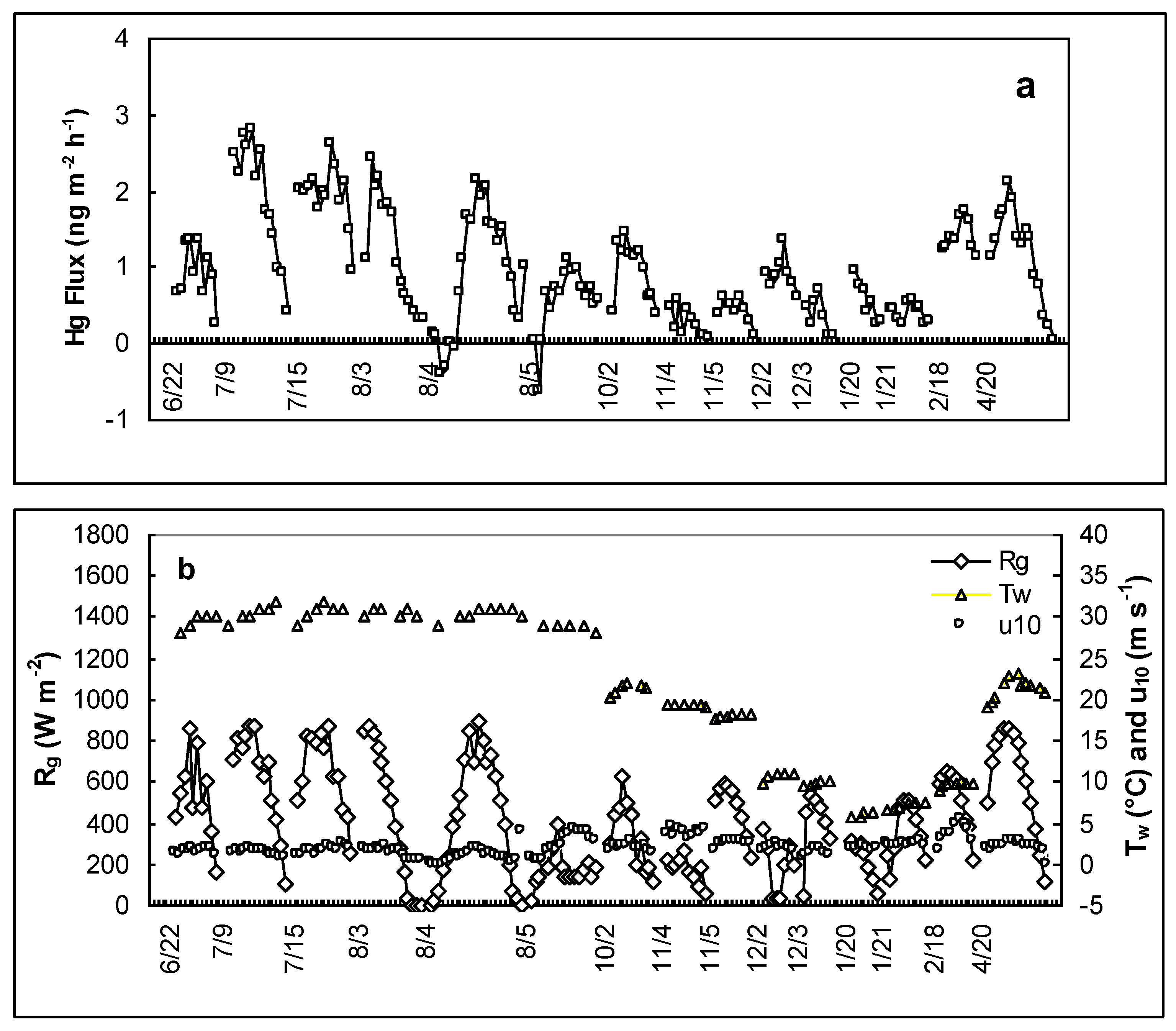
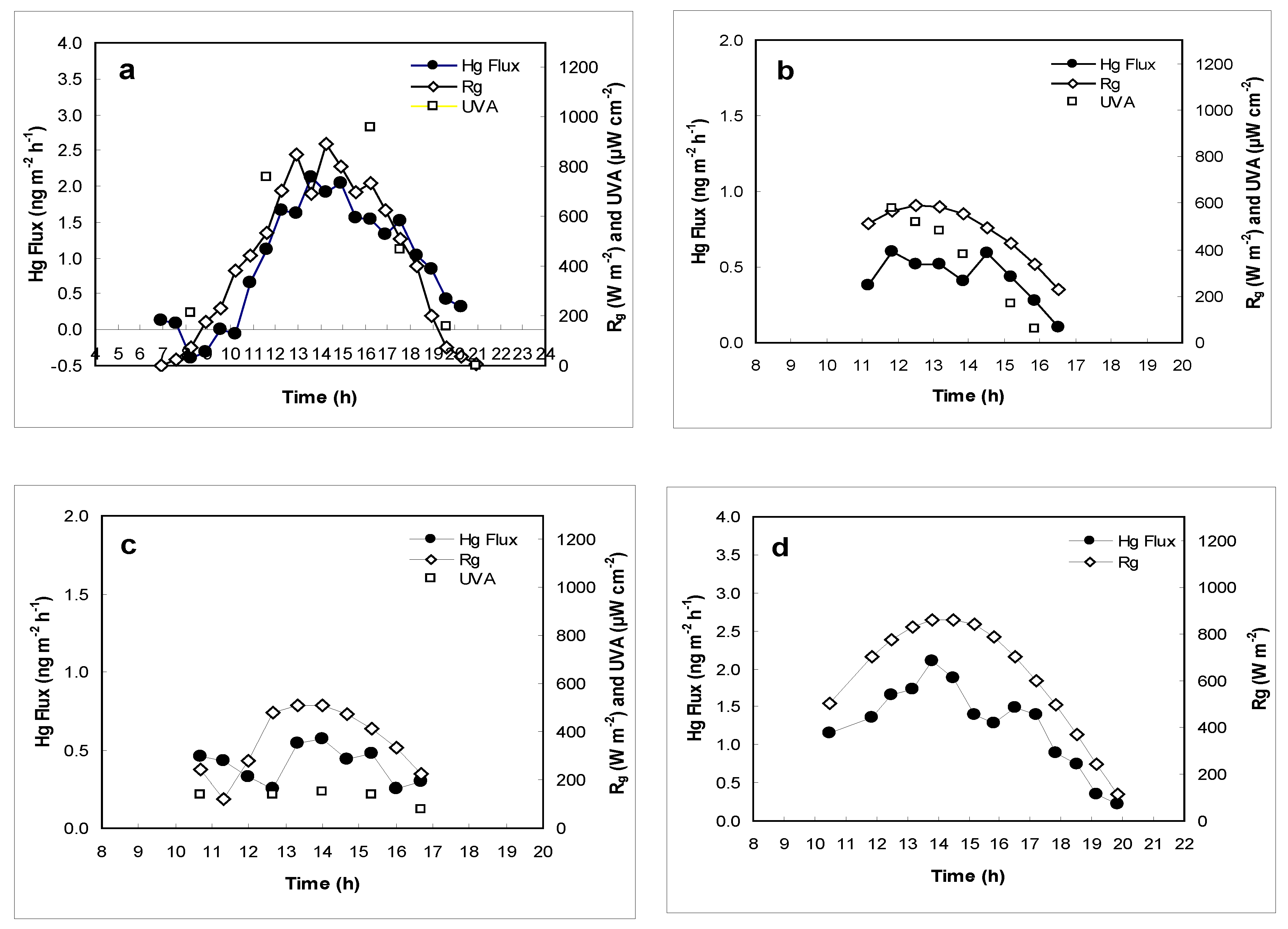
3.1. Daily Magnitude and Variation of Hg Air/Water Exchange Flux

The magnitude of the Hg air/water exchange flux over Cane Creek Lake was obtained for each of the sampling days, and a summary of the flux results together with the meteorological data is presented in Table 2 and Figure 1. The values for the first period of the field study (June–August) are significantly higher than those for the next one (October–January). For the months of June through August, the average daily flux values ranged at 0.92–1.9 ng m⁻² h⁻¹, and the maximum daily flux values were 1.1–2.8 ng m⁻² h⁻¹ (Table 2). During the later months (October through January), the flux values were lower; during this period, the average daily flux values were 0.27–0.95 ng m⁻² h⁻¹, and the maximum daily flux values were 0.57–1.4 ng m⁻² h⁻¹. An exception was 2 December, which had a daily average of 0.91 ng m⁻² h⁻¹ and a maximum value of 1.4 ng m⁻² h⁻¹. The fluxes went up afterwards through the spring (March–April) of the following year with the daily fluxes as high as 2.1 ng m⁻² h⁻¹ in April (Table 2).

Some negative fluxes were observed in the present study. However, during the entire nearly year-long field study, the negative fluxes occurred only in a single case in which a continuous flux measurement field campaign was conducted to obtain 24 h diel flux cycles during the period of 3–5 August (Table 2, Figure 1a) and this particular study was undertaken at the secondary site as mentioned previously. This case is interesting, but it is rather not straightforward to interpret this observation, especially in the consideration that it occurred only on the secondary site and in a special occasion in the morning times of 4 and 5 August (Figure 1a). Nevertheless, if this observation is assumed to be a real phenomenon, then its occurrence could be due to a build-up of the air Hg(0) concentration overnight above the water surface as the wind calmed down, or an effective drop of the dissolved gaseous mercury (DGM) concentration in the surface water, or both, since these changes could reverse the Hg(0) concentration gradient across the air/water interface, causing the negative fluxes. It is well-known that the DGM concentration can decrease to great degrees from mid-afternoon through the night to the morning time (e.g., see [10] and references within). This trend was also clearly observed on the very same site in a previous field study to characterize the DGM trends in Cane Creek Lake [19,30].

A comparison of the emission flux values observed for Cane Creek Lake with the results of the previously published studies is of interest. Table 1 presents some previous results of the Hg emission fluxes mainly for northern America regions (with some for northern Europe, e.g., see [26]), which share similar conditions for environmental Hg pollution. O’Driscoll et al. [10], for example, observed Hg emissions from two Canadian lakes and the emission fluxes found ranged from −4.6 to 9 ng m⁻² h⁻¹ for one lake and −0.15 to 6.5 ng m⁻² h⁻¹ for the other. Gardfeldt et al. [9] reported an average flux of 11 ng m⁻² h⁻¹ for a river in southwestern Sweden. The maximum values in the summer for Cane Creek Lake reached only 2.8 ng m⁻² h⁻¹, far lower than the flux values observed by O’Driscoll et al. [10] and Gardfeldt et al. [9]. Lindberg and Zhang [23] reported the Hg emission fluxes in the Florida Everglades; the average daily fluxes in the summer were 3 ± 2 ng m⁻² h⁻¹, and the fall and winter average values were 2 ± 4 ng m⁻² h⁻¹. These results are comparable to those we observed at Cane Creek Lake. Poissant and Casimir [24] observed the emission fluxes of −0.5–1.0 ng m⁻² h⁻¹ over the St. Lawrence River, and these results are somewhat lower than ours observed at Cane Creek Lake. It appears that no clear geographic trends of the Hg air/water exchange fluxes are recognizable among the published data available so far.

The emission fluxes at Cane Creek Lake frequently exhibited diurnal patterns that closely followed the solar radiation variations. Typical examples of these patterns were found on 9 July [29], August 3 [29], August 4 (Figure 2a), October 29 [29], and November 5 (Figure 2b), and April (Figure 2d). For example, a typical full diurnal flux pattern was observed on August 4. The flux plot for the day (Figure 2a) shows the peak of the emission fluxes around 1:30 pm with the emission increasing in the morning and decreasing in the afternoon and evening hours. The solar radiation on the same day exhibited a similar trend (Figure 2a). The plot of the diurnal flux pattern for 29 October shows the peak around 1:30 pm [29] and that for 4 April 2005 around 1:45 pm (Figure 2d).

O’Driscoll et al. [10] observed typical diel patterns of the Hg emission fluxes for both lakes of Canada studied as mentioned previously. The peaks appeared near the middle of the day with the fluxes rising in the morning and falling in the afternoon and evening, following the solar radiation variation closely. The daily emission flux and solar radiation at the Everglades (FL, USA) also showed strong diurnal patterns [23], exhibiting the same trends observed by O’Driscoll et al. [10]. An extensive study by Zhang et al. [25] also showed the typical diel trends over the wetlands in the Bay Saint Francois of Canada. Similar diurnal patterns for the Hg emission fluxes were also observed elsewhere (e.g., [4,9,12,24,27], showing flux increase in the morning and decrease in the afternoon and evening hours.

The patterns of the Hg emission flux variations other than the typical diurnal patterns as shown above were also observed at Cane Creek Lake in this study as shown by the following examples [29]. For instance, the data for 15 July show delayed flux peak around 3:45 pm. The data for 5 August show low solar radiation with a flux curve that does not match the solar radiation closely, and the fluxes exhibit a delayed peak around 2:45 pm. On 4 November, both the Hg emission flux and solar radiation showed high variations. The data for 2 December is interesting. The peak for the emission flux occurred at the same time as the solar radiation reached its lowest values, which is opposite to what is expected. The data for 3 December show little parallel between the emission flux and solar radiation (Figure 1 and data shown in [29]). These findings demonstrate that the Hg emission fluxes may also be subject to the controls other than solar radiation.

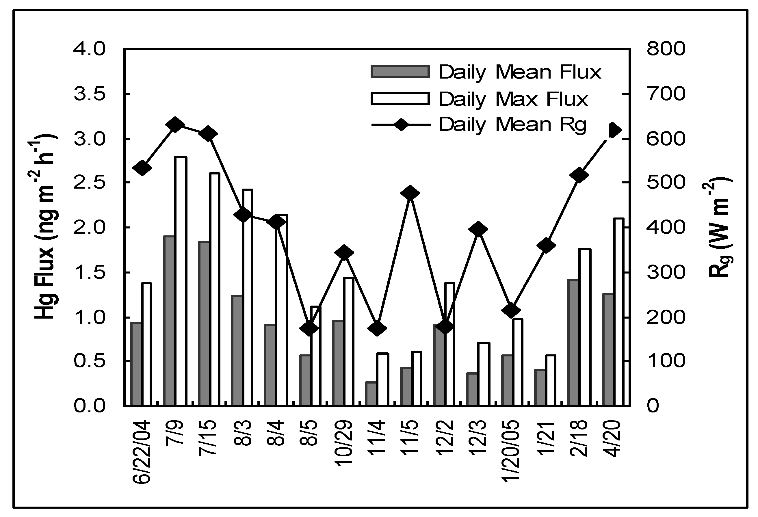
3.2. Seasonal Trends of Hg Air/Water Exchange Flux

The seasonal trend of the Hg emission fluxes at Cane Creek Lake is presented in Figure 3 and Table 3. Figure 3 shows the average and maximum daily flux values plotted with the daily average solar radiation (R_g) for the entire study period from June to April. A seasonal trend of the Hg emission fluxes emerges that although fluctuating, the fluxes generally were high in the summer months (June–August) and low in the fall (September–November) and winter (December–February) months followed by a bounce back in the springtime (March–April); moreover, this flux trend also generally follows the seasonal variation of solar radiation (Figure 3). This trend of the Hg flux variation mirrors the daily flux change patterns presented previously (Figure 1 and Figure 2). Thus, the effect of solar radiation on the Hg air/water exchange manifests on both the daily and seasonal scales.

The seasonal Hg emission flux trend is also reflected by the seasonal means of the fluxes (Table 3). The mean flux value for the summertime (1.2 ng m⁻² h⁻¹) nearly doubles that for the fall time (0.6 ng m⁻² h⁻¹) and the wintertime (0.7 ng m⁻² h⁻¹). The same trend holds true for the seasonal maximum fluxes (Table 3). These trends correlate with the seasonal mean values of solar radiation with respect to R_g and UVA (Table 3).

The daily and seasonal trends of the Hg air/water exchange fluxes observed at Cane Creek Lake share the daily and seasonal trends of the DGM concentrations in the same lake observed in our previous study [19,22,28]. This similarity seems to support the two-thin film model (TTF model) for Hg air/water exchange as formulated below [4,10,13,25,29,33,34]:

$$F=k_w\left[C_w-\frac{C_a}{K_H{}^{\prime }}\right]$$

(3)

where, F is the emission flux from the water (ng m⁻² h⁻¹), k_w is the gas transfer coefficient (m h⁻¹), C_w is the concentration of Hg in the water (DGM, ng m⁻³), C_a is the concentration of Hg in the ambient air above the water (ng m⁻³), and K_H′ is Henry’s law constant (dimensionless, depending on water temperature). The above model equation indicates that the Hg air/water exchange flux should depend approximately linearly on the concentration of DGM; in other words, the above equation prescribes the similar trend shared by the Hg air/water exchange and DGM. Our calculations showed that the model-predicted results agreed satisfactorily or acceptably with the measured flux values in trends for various cases, although not in every case [29]. A detailed description of the use of the TTF model in predicting the Hg emission fluxes from the Cane Creek Lake water is given subsequently in Section 3.6.

It needs to be pointed out that the apparent linear dependence of the Hg flux on the DGM concentration is based on the assumption that k_w, C_a, and K_H′ remain approximately constant (i.e., varying slowly compared to the change of DGM). This assumption is roughly valid, especially with respect to C_a and K_H′, since C_a varied only slightly (data not shown, see [29]) and the site temperature (thus K_H′) changed only moderately (Table 2). The two-thin film model is instructive in discussing the factors that control the Hg air/water exchange. It indicates that the Hg air/water exchange is dependent also on k_w, which in turn depends on solar radiation and wind speed. Hence, the assumption of a constant k_w is probably not quite valid since both solar radiation and wind speed are highly variable. Therefore, the Hg air/water exchange is also subject to the control of solar radiation and wind speed. These effects will be discussed below.

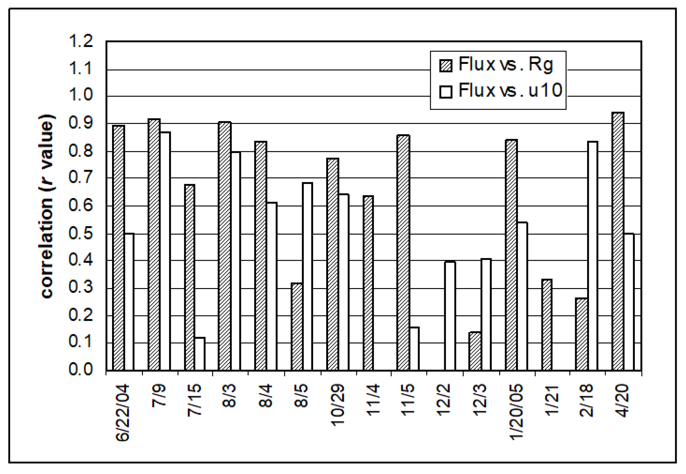
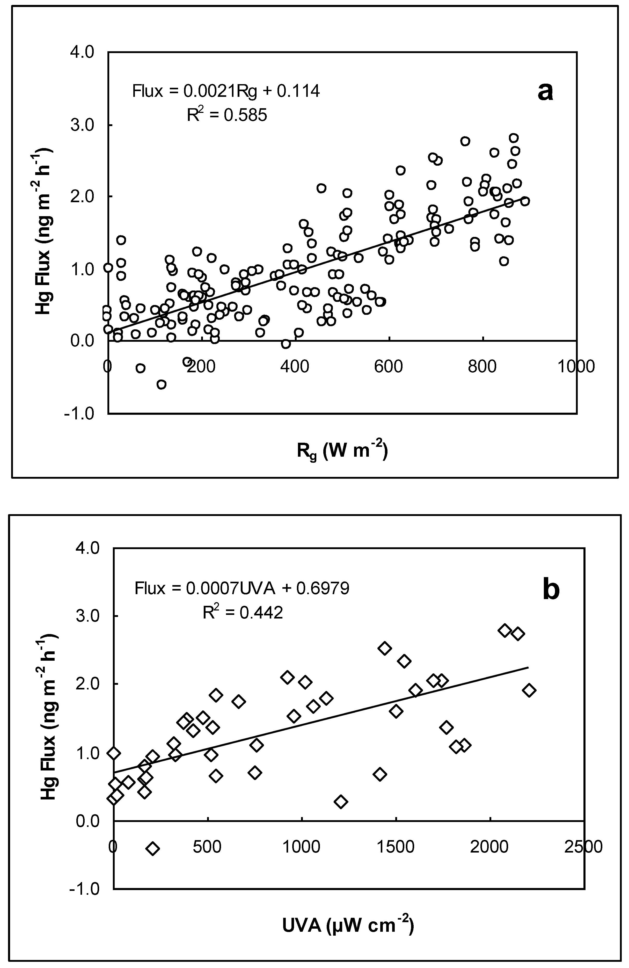
3.3. Effect of Solar Radiation on Hg Air/Water Exchange

Solar radiation has been shown to enhance Hg air/water exchange over various aquatic systems (e.g., see [9,10,23,24]). Our study at Cane Creek Lake supports this notion in various cases. For some days at the lake, the Hg air/water exchange fluxes appeared to follow the solar radiation (R_g) exhibiting typical diurnal trends. The data of July 9, for example, gives a good correlation between the two (r = 0.9208, p < 0.0005); the same is true for the data of 3 August (r = 0.9033, p < 0.0005) and 4 August (r = 0.8366, p < 0.002), and 20 April (r = 0.9434, p < 0.0005). Correlations were also found for the data of 5 November (r = 0.8567, p = 0.002) and 20 January (r = 0.8402, p = 0.002).

Three days of the field measurements exhibited good correlations between the Hg flux and solar radiation, but did not show the typical diurnal trends of the morning rise and afternoon fall in fluxes. The data of 22 June give the correlation value of r = 0.8930 (p < 0.0005) without the diurnal rise and fall of fluxes, and the same can be seen for 15 July (r = 0.6768, p = 0.027) and October 29 (r = 0.7736, p = 0.01) [29]. The data of some days did not show any significant correlation between the emission flux and solar radiation (e.g., 5 August, 2 and 3 December, and 21 January) [29]. A complete presentation of the correlations between the Hg fluxes and R_g for this study is given in Figure 4.

The relationship between the Hg air/water exchange flux and solar radiation was also inspected on the seasonal scale. The daily mean and maximum emission fluxes correlate with the daily mean solar radiation in terms of R_g (r = 0.7086, p = 0.004 and r = 0.6318, p = 0.012, respectively) considering all the days of field measurements over the entire study period; the daily maximum emission fluxes also correlate with the daily maximum R_g values (r = 0.7916, p = 0.007). Similarly, the daily mean and maximum emission fluxes correlate with the daily mean UVA radiation (r = 0.8510, p = 0.002 and r = 0.7928, p = 0.007, respectively); the daily maximum emission fluxes also correlate with the daily maximum UVA radiation (r = 0.8505, p = 0.002). The relationship between all individual emission flux points versus the solar radiation data (R_g and UVA) are presented in Figure 5. With all the data considered together, general correlating trends of the flux vs. R_g and UVA can be recognized by ignoring the fluctuations as shown in Figure 5. These results show that the Hg air/water exchange fluxes increase with the increase of solar radiation. Our study thus supports the notion that solar radiation exerts a strong control over the Hg air/water exchange in aquatic systems.

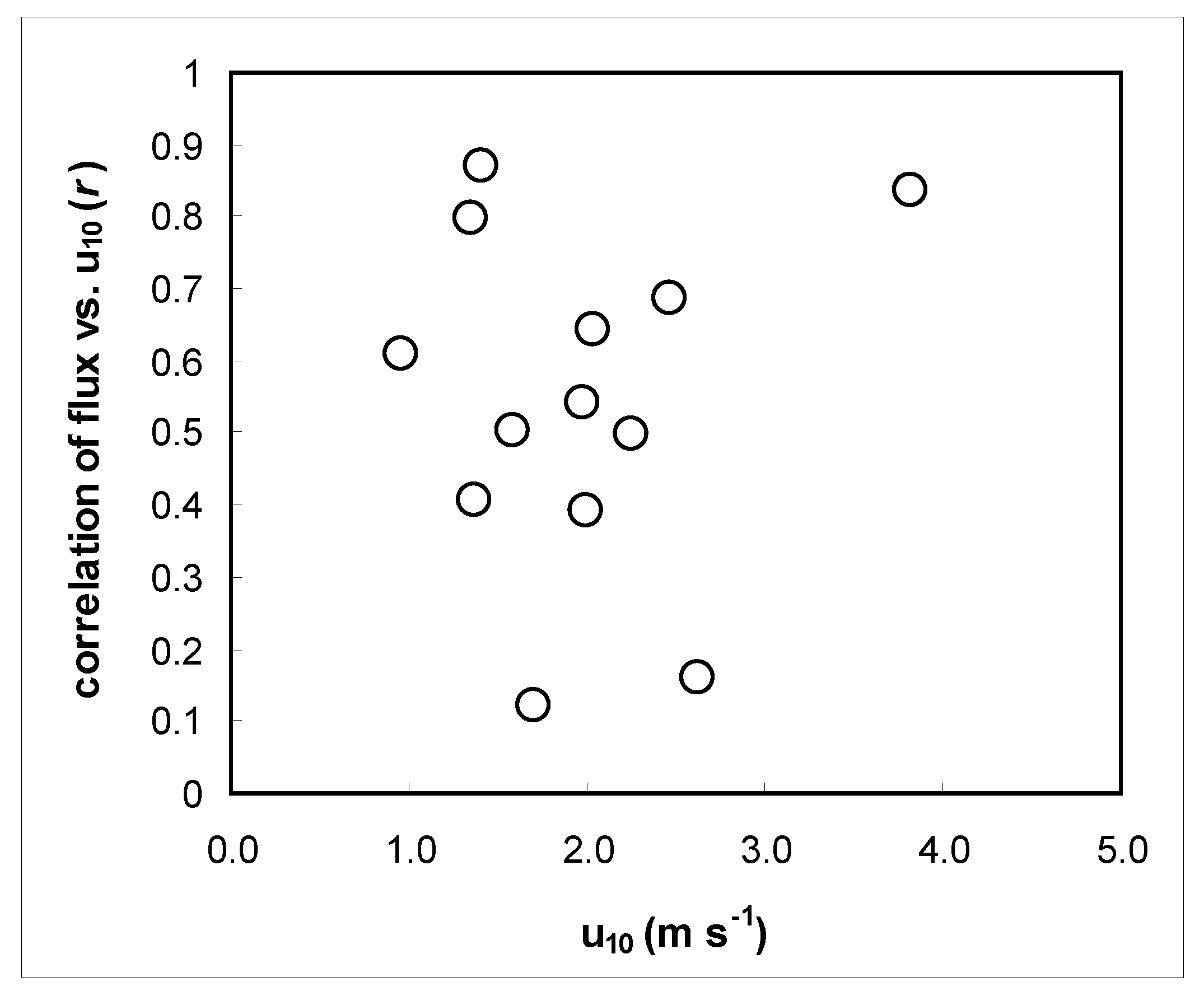
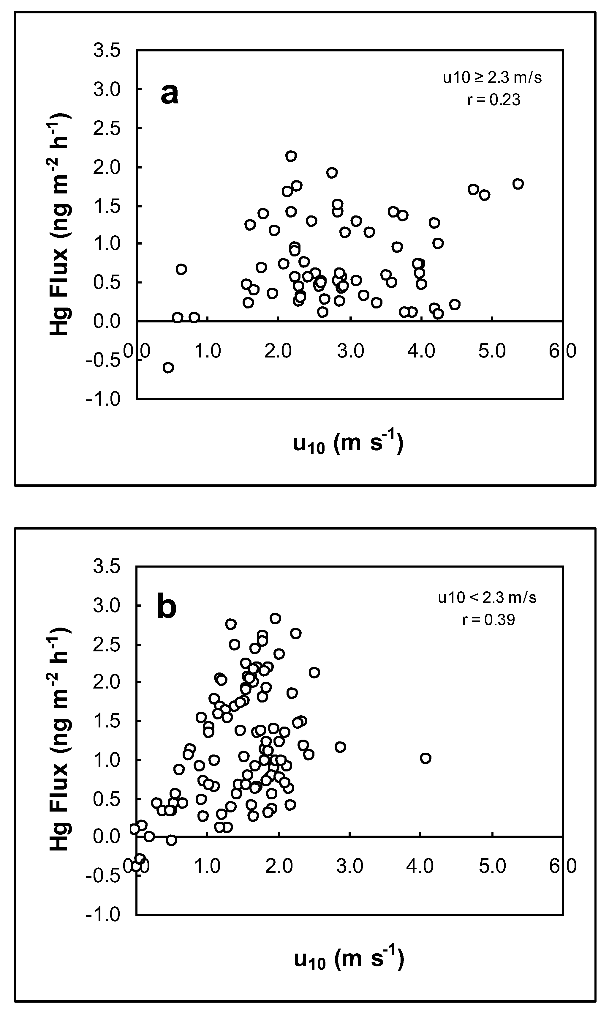
3.4. Effect of Wind on Hg Air/Water Exchange

According to the two-thin film model, the effect of wind on the air/water interface should influence the magnitude of the Hg air/water exchange. Wind speed is related to the gas transfer coefficient and can affect the emission flux in linear [35] and non-linear [29] manners. The wind over water can disturb the air/water interface through waves, and the breaking waves accelerate the gas transfer from the water into the air [36]. Attempts were thus made to examine the effect of the wind speed on the Hg air/water exchange over Cane Creek Lake.

The modified wind speed values (adjusted to 10 m above the water surface, u₁₀) are provided in Table 2 and Table 3. The average wind speed for the summer (June–August) was 1.6 m s⁻¹, which is lower than the average wind speed of 2.6 m s⁻¹ for the fall and winter months (October–February). This is opposite to the trend for solar radiation (Table 2 and Table 3). Small variations were seen for the wind speed (low standard deviations, generally SD < 0.8 m s⁻¹) except for 4 August (SD = 0.97 m s⁻¹) and 5 August (SD = 1.4 m s⁻¹). Figure 4 shows the correlations between the Hg air/water exchange fluxes and the wind speed values (u₁₀). The trends are inconsistent and the correlations appear to exhibit no dependence on the wind speed (Figure 4 and Figure 6). Both significant (e.g., r = 0.8694, p = 0.001 on 9 July, r = 0.7986, p = 0.007 on 3 August, r = 0.8370, p = 0.003 on 18 February) and poor correlations were found across the seasons. In a few cases, the correlations were even negative (e.g., r = –0.4528 on 4 November, r = –0.1590 on 21 January).

In some cases, the apparent correlating trends were observed, but the corresponding p values were high. For example, on July 15 the emission flux appeared to follow the variation in the wind speed (Figure 1 and [29]), but the p value is 0.741. The emission flux and wind speed shared the similar trends on 2 and 3 December (Figure 1 and [29]), yet the p values in both cases are high (0.265 and 0.252, respectively).

The relationship between the Hg air/water exchange flux and wind speed (u₁₀) on a seasonal scale, however, is different completely from that on a daily scale. The correlations of the daily mean and maximum Hg air/water exchange fluxes and the daily mean wind speeds were found to be negative considering all the sampling days over the entire study period; the same is true for the correlation between the daily maximum Hg fluxes and the daily maximum wind speeds. This suggests that the effect of the wind speed differs from that of the solar radiation and seems to be more complicated. The relationship between all individual emission flux points versus the wind speeds (u₁₀) are presented available in SM Figure S1. This figure further reinforces the notion that the effect of the wind speed on the Hg air/water exchange is indeed complicated.

Boudala et al. [27] reported a positive correlation between the Hg air/surface exchange fluxes and wind speeds (r² = 0.45) over Big Dam West Lake (Canada). Similar findings were also reported for the sites (WCA2A in summer and Cell 3 in winter) at the Florida Everglades [23]. Boudala et al. [27] further showed that significant increases in the Hg flux with increasing of the wind speed occurred at the wind speed >~2 m s⁻¹ as observed by others. Our data from this study, however, show that the Hg fluxes increased clearly with the increase of the wind speed at the daily mean wind speed <2.3 m s⁻¹, while there was no clear increase or other trend found for the case with the daily mean wind speed >2.3 m s⁻¹ (Figure 7). Actually, the correlation between the Hg flux and wind speed seems somewhat better for the case with the daily mean wind speed <2.3 m s⁻¹ than for the case with ≥ 2.3 m s⁻¹ (Figure 7). Our data (Figure 7) also supports the notion that the formation of the sub-surface layer (surface air layer <100 cm above) of strong stability linked to Hg evasion is in good agreement with the relationship between low wind speeds and higher Hg evasion [24]. Although wind can enhance the Hg air/water exchange by increasing the rate of the transport of Hg(0) through vertical mixing, this mechanism cannot act alone to account for the increase of the Hg flux with increasing of the wind speed and the role of solar radiation also needs to be considered [27]. It is likely that these two factors are intertwined. In other words, wind and heat conditions are probably inter-related and so the Hg air/water exchange responds to the effect of both solar radiation and wind. A comparison of the effects of solar radiation and wind speed from further investigation thus should be of interest.

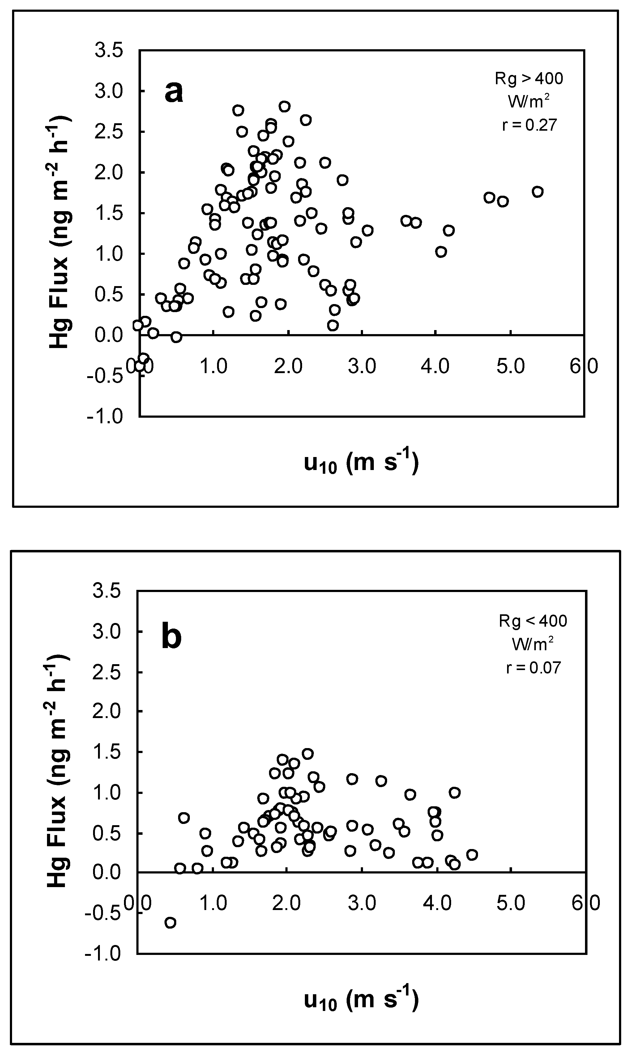
3.5. Comparison of Effects of Solar Radiation and Wind Speed on Hg Air/Water Exchange

The previous analyses show that generally the Hg air/water exchange fluxes correlate better and more consistently on both daily and seasonal scales with solar radiation (R_g and UVA) than with the wind speed (u₁₀) (Figure 4 and Figure 5). This suggests that solar radiation appears to play a primary role in controlling the magnitude and trend of the Hg air/water exchange over the lake studied. This notion is supported by the observations that the wind speeds were highest on 4 and 5 November and 21 January (Table 2), but the daily mean Hg fluxes for the same days were among the lowest. Interestingly, our data also show that the correlation between the Hg fluxes and wind speeds appears to be better for the data with the daily mean solar radiation >400 W m⁻² than the data with the daily mean solar radiation <400 W m⁻² (Figure 8). The effect of wind may manifest through wind-induced transport and supply of photochemically reducible Hg(II) species to the water surface [27]. Thus, wind and solar radiation jointly enhance the Hg air/water exchange, although there seems to be no correlation between solar radiation (R_g) and wind speed (u₁₀) (SM Figure S2).

The dynamic flux chamber system does protect the surface water from the direct wind effects, but the wave caused by the wind still could reach into the chamber. Although the mixing of water should enhance the transfer of gases through the water, this phenomenon is not supported by our Hg air/water exchange flux measurements in this study. Our study seems to support the idea that wind probably plays a secondary role in controlling the Hg air/water exchange over the lake in this study. This notion also agrees well with the similar findings reported previously (e.g., see [23,24,27]). Further research to investigate the effect of wind on Hg air/water exchange in various aquatic systems should shed more light on the role of wind in controlling Hg air/water exchange.

3.6. Calculation of Hg Fluxes Using the Two-Thin-Film Theory

To further extend and enhance the discussion of the Hg air/water exchange flux results, the two-thin-film model as discussed previously in Section 3.2 (TTF theory) was used to calculate the Hg fluxes from the Cane Creek Lake water. This serves as an effort towards a full use of the field data collected in this field study, rather than as an attempt to validate the TTF model, which is beyond the scope of this field study and the present research report. The TTF theory has been widely used for estimating Hg emission from freshwaters (e.g., see [29] and references within) and also from salty waters, such as estuaries and coastal lagoons (e.g., see [37]). The model equation has been given previously as Equation 3. This is the general model equation that is employed to calculate the Hg air/water exchange fluxes by using coupled concentrations of DGM (C_w) and air Hg (C_a). The only model parameter in the model equation is k_w, the gas transfer coefficient (m h⁻¹), which is dependent on the assumptions made about the nature of the Hg exchange at the air/water interface (the two-thin-film). In the present work, four previously published models for this parameter were used to calculate the Hg fluxes as described below.

Model 1:

k_w1 = 0.09 m h⁻¹

(4)

The gas transfer coefficient in this model is a constant without a consideration of wind speed [24].

Model 2

$$k_{w2}=0.0017u_{10}{\left[\frac{S{c}_{\mathrm{H}\mathrm{g}}}{S{c}_{C{O}_2}}\right]}^{-0.5}\mathrm{for} u_{10}<3.6 {\mathrm{m}\mathrm{s}}^{-1}$$

(5)

$$k_{w2}=\left(0.0285u_{10}-0.0965\right){\left[\frac{S{c}_{\mathrm{H}\mathrm{g}}}{S{c}_{C{O}_2}}\right]}^{-0.5} \mathrm{for}3.6<u_{10}<13 {\mathrm{m}\mathrm{s}}^{-1}$$

(6)

$$k_{w2}=\left(0.059u_{10}-0.493\right){\left[\frac{S{c}_{\mathrm{H}\mathrm{g}}}{S{c}_{C{O}_2}}\right]}^{-0.5}\mathrm{for}{u}_{10}>13 {\mathrm{m}\mathrm{s}}^{-1}$$

(7)

where Sc is the Schmidt number and u₁₀ is the wind speed at 10 m above the air/water interface. The gas transfer coefficient in this model follows the Liss and Merlivat linear expression with respect to wind speed [35].

Model 3:

$$k_{w3}=0.0031u_{10}{}^2{\left[\frac{S{c}_{\mathrm{H}\mathrm{g}}}{S{c}_{C{O}_2}}\right]}^{-0.5}$$

(8)

The gas transfer coefficient in this model follows the Wanninkhof non-linear equation with respect to the wind speed [23,32].

Model 4:

$$k_{w4}=0.0036+51.84u_{10}{}^{2.2}S{c}_{Hg}{}^{-0.5}$$

(9)

The gas transfer coefficient in this model takes a form of a modified linear equation with respect to the wind speed [4,10].

Each of the above model parameters of k_w was then inserted into the general TTF model equation (Equation (3)) to generate four individual TTF model equations. These were then used to implement the calculation of the Hg emission fluxes. The coupled DGM concentration (C_w) and air Hg concentration (C_a) together with the corresponding water temperature (for corresponding K_H′, Henry’s law constant) obtained in the fieldwork in parallel to the field flux measurement were used in the flux calculations. The flux calculation results were then used to find which model(s) would work for the studied lake in reproducing the Hg fluxes from the lake water. This is the major goal for this flux calculation exercise.

A brief description of the flux calculation outcome is as follows. The main difference in the flux results for various models is the magnitude of the emission flux values reflecting the varying gas transfer coefficient used. Generally, the calculated flux results predicted by Model 4 are greater than those by the other models by two orders of magnitude. The flux values given by Models 2 and 3 are significantly smaller than the other model values, while the flux results by Model 1 vary greatly. Yet, despite the differences in the calculated flux magnitude, there are some similarities in the overall shapes and trends of the calculated fluxes for the various models used.

The model-calculated Hg emission fluxes were then compared with the corresponding field-measured fluxes in order to find which model(s) would work to reproduce the Hg emission fluxes from the Cane Creek Lake water. Generally speaking, Models 1 and 4 overestimate the emission flux. The gas transfer coefficients for Models 1 and 4 are too large, making the flux values too high as compared to the measured flux values. Recent determinations of the elemental Hg diffusion coefficient by molecular dynamics simulation [38] and by experimental measurement [39] show that the newly determined Hg diffusion coefficients are actually lower than those used in some previous flux prediction models. Models 2 and 3, however, give an underestimation of the emission fluxes.

To obtain an overall picture of the model performance collectively, two statistical methods were used to inspect the differences between the calculated and measured flux values, i.e., the average residual values and the root mean squared errors (RMSE). As a simple way to estimate the flux differences, the residual value is merely the difference between the modeled and calculated flux values [10]:

Residual = Modeled Flux − Measured Flux

(10)

The RMSE is a sophisticated statistical way of estimating the flux differences and can be calculated using the following equation [40]:

$$\mathrm{RMSE}=\sqrt{\left[\frac{1}{n_d-n_p}\right]{\displaystyle \sum }_{j=1}^{n_d}{\left(C_j-C_j{}^{\prime }\right)}^2}$$

(11)

where n_d is the number of data points, n_p is the number of adjustable parameters, C_j and C_j′ are the measured and modeled fluxes, respectively. The models that best fit or reproduce the measured flux values should have the lowest absolute average residuals and lowest RMSE values. The statistical calculations show that the lowest RMSE values occur to Model 3 (

Table 4. The results of the Root Mean Squared Errors (RMSE) used to inspect the differences between the model-calculated fluxes and the field-measured fluxes using various models (Models 0–4).

		RMSE
Date	Model 0	Model 1	Model 2	Model 3	Model 4
22 June 2004	3.5	1.1	1.0	1.0	115.1
9 July 2004	3.0	3.9	2.0	1.6	536.6
15 July 2004	2.9	1.1	2.2	2.1	109.4
3 August 2004	3.7	1.4	2.0	1.8	205.5
4 August 2004	2.3	1.2	1.4	1.3	175.2
5 August 2004	3.1	0.5	0.8	0.7	89.2
29 October 2004	3.8	0.9	1.1	1.0	122.1
5 November 2004	5.3	1.4	0.4	0.3	338.3
3 December 2004	2.9	3.3	0.4	0.3	165.4
21 January 2005	4.2	2.3	0.3	0.1	347.3
Mean RMSE	3.5	1.7	1.2	1.0	220.4

Model 0: Empirical Model [10]. Model 1: [24]. Model 2: [35]. Model 3: [23,32]. Model 4: [4,10].

). The same consistently holds true for the inspection using the absolute average residuals [29]. This seems to suggest that Model 3 would yield the fluxes closest to the measured flux values for the Cane Creek Lake water. More research would be needed to further sophistically evaluate the applicability of the models in predicting Hg air/water exchange from lakes. One additional interesting finding worth mentioning here is that both the average residual and the RMSE values in the summertime (June–August) are higher than in the wintertime (December–February).

In addition to the TTF models, an empirical equation (Model 0, a non-TTF model) relating the solar radiation and wind speed to the Hg emission flux as given below [10] was also used to evaluate its use in predicting the Hg emission fluxes from the lake water.

F = 2.44R_gu₁₀^1.5 + 1.1

(12)

where F is the emission flux in ng m⁻² h⁻¹, R_g is the global solar radiation in W m⁻², and u₁₀ is the wind speed at 10 m above the air/water interface in m s⁻¹. The flux calculations using the empirical model show that this model yields flux estimates higher than those by Models 2 and 3 for the TTF model. It appears that the empirical model is probably best applicable to a large water body with high wind speeds, not characteristic of Cane Creek Lake in the present study. A detailed presentation of the performance of all the models (Models 1–4 and empirical model) in predicting the Hg emission fluxes from the Cane Creek Lake water is available elsewhere [29].

4. Summary and Conclusions

Our year-long field study on the Hg air/water exchange at Cane Creek Lake (TN, USA) shows that the Hg exchange over the lake generally exhibits diurnal patterns closely following the change of solar radiation. However, there are various cases that deviate from this daily flux trend. The Hg emission fluxes are all below 3 ng m⁻² h⁻¹ and the daily mean fluxes are below 2 ng m⁻² h⁻¹. There seem to be no clear geographic trends of the Hg air/water exchange fluxes recognizable among the data available so far. The Hg emission fluxes of the lake are higher in the summer than in the fall and winter. The daily and seasonal trends of the Hg air/water exchange flux changes are similar to the trends of the changes of the dissolved gaseous mercury (DGM) concentrations in the lake observed in our previous study. Solar radiation appears to be the primary factor controlling the Hg air/water exchange. Wind speed exerts a secondary effect on the transfer of Hg from the water to the air. Among the four two-thin-film model equations used to calculate the Hg emission fluxes from the lake water, the Wanninkhof non-linear gas transfer model appears to yield the results closest to the field-measured flux values obtained using the DFC method in the present study.

References

1. Mason, R.P.; Fitzgerald, W.F.; Morel, F.M.M. The biogeochemical cycling of elemental mercury: Anthropogenic influences. Geochim. Cosmochim. Acta 1994, 58, 3191–3198. [Google Scholar] [CrossRef]
2. Schroeder, W.H.; Munthe, J. Atmospheric Mercury—An Overview. Atmos. Environ. 1998, 32, 809–822. [Google Scholar] [CrossRef]
3. Sommar, J.; Osterwalder, S.; Zhu, W. Recent advances in understanding and measurement of Hg in the environment: Surface-atmosphere exchange of gaseous elemental mercury (Hg0). Sci. Total Environ. 2020, 721, 137648. [Google Scholar] [CrossRef] [PubMed]
4. Xu, X.; Yang, X.; Miller, D.R.; Helble, J.J.; Carley, R.J. Formulation of bi-directional atmosphere-surface exchanges of elemental mercury. Atmos. Environ. 1999, 33, 4345–4355. [Google Scholar] [CrossRef]
5. Amyot, M.; Mierle, G.; Lean, D.R.; McQueen, D.J. Sunlight-induced formation of dissolved gaseous mercury in lake waters. Environ. Sci. Technol. 1994, 28, 2366–2371. [Google Scholar] [CrossRef]
6. Amyot, M.; Lean, D.; Mierle, G. Photochemical formation of volatile mercury in high arctic lakes. Environ. Toxicol. Chem. 16, 2054–2063. [CrossRef]
7. Amyot, M.; Mierle, G.; Lean, D.; McQueen, D.J. Effects of solar radiation on the formation of dissolved gaseous mercury in temperate lakes. Geochim. Cosmochim. Acta 1997, 61, 975–987. [Google Scholar] [CrossRef]
8. Costa, M.; Liss, P.S. Photoreduction of mercury in sea water and its possible implications for Hg0 air/sea fluxes. Mar. Chem. 1999, 68, 87–95. [Google Scholar] [CrossRef]
9. Gardfeldt, K.; Feng, X.; Sommar, J.; Lindqvist, O. Total gaseous mercury exchange between air and water at river and sea surface in Swedish coastal regions. Atmos. Environ. 2001, 35, 3027–3038. [Google Scholar] [CrossRef]
10. O’Driscoll, N.J.; Beauchamp, S.; Siciliano, S.D.; Rencz, A.N.; Lean, D.R.S. Continuous analysis of dissolved gaseous mercury (DGM) and mercury flux in two freshwater lakes in Kejimkujik Park, Nova Scotia: Evaluating mercury flux models with quantitative data. Environ. Sci. Technol. 2003, 37, 2226–2235. [Google Scholar]
11. Fitzgerald, W.F.; Mason, R.P.; Vandal, G.M. Atmospheric cycling and air-water exchange of mercury over mid-continental regions. Water Air Soil Poll. 1991, 56, 745–767. [Google Scholar] [CrossRef]
12. Poissant, L.; Amyot, M.; Pilote, M.; Lean, D. Mercury water-air exchange over the upper St. Lawrence river and Lake Ontario. Environ. Sci. Technol. 2000, 34, 3069–3078. [Google Scholar] [CrossRef]
13. Vandal, G.M.; Mason, R.P.; Fitzgerald, W.F. Cycling of volatile mercury in temperate lakes. Water Air Soil Poll. 1991, 56, 791–803. [Google Scholar] [CrossRef]
14. Vette, A.F. Photochemical Influences on the Air-Water Exchange of Mercury. Ph.D. Thesis, University of Michigan, Ann Arbor, MI, USA, August 1998. [Google Scholar]
15. Zhang, H.; Lindberg, S.E. Sunlight and iron (III)-induced photochemical production of dissolved gaseous mercury in freshwater. Environ. Sci. Technol. 2001, 35, 928–935. [Google Scholar] [CrossRef]
16. Nriagu, J.O. Mechanistic steps in the photoreduction of mercury in natural waters. Sci. Total Environ. 1994, 154, 1–8. [Google Scholar] [CrossRef] [Green Version]
17. Xiao, Z.F.; Stromberg, D.; Lindqvist, O. Influence of humic substances on photolysis of divalent mercury in aqueous solution. Water Air Soil Poll. 1995, 80, 789–798. [Google Scholar] [CrossRef]
18. Zhang, H. Photochemical redox reactions of mercury. In Recent Developments in Mercury Science; Atwood, D.A., Ed.; Structure and Bonding series; Springer: Berlin, Germany, 2006; Volume 120, pp. 37–79. [Google Scholar]
19. Dill, C.; Kuiken, T.; Zhang, H.; Ensor, M. Diurnal variation of dissolved gaseous mercury (DGM) levels in a southern reservoir lake (Tennessee, USA) in relation to solar radiation. Sci. Total Environ. 2006, 357, 176–193. [Google Scholar] [CrossRef]
20. O’Driscoll, N.J.; Lean, D.R.S.; Loseto, L.L.; Carignan, R.; Siciliano, S.D. Effect of dissolved organic carbon on the photoproduction of dissolved gaseous mercury in lakes: Potential impacts of forestry. Environ. Sci. Technol. 2004, 38, 2664–2672. [Google Scholar] [CrossRef]
21. Zhang, H.; Lindberg, S.E. Trends in dissolved gaseous mercury in the Tahquamenon river watershed and nearshore water of Whitefish bay in the Michigan Upper Peninsula. Water Air Soil Poll. 2002, 133, 381–391. [Google Scholar] [CrossRef]
22. Zhang, H.; Dill, C.; Kuiken, T.; Ensor, M.; Crocker, W. Change of dissolved gaseous mercury (DGM) concentrations in a southern reservoir lake (Tennessee, USA) following seasonal variation of solar radiation. Environ. Sci. Technol. 2006, 40, 2114–2119. [Google Scholar] [CrossRef]
23. Lindberg, S.; Zhang, H. Air/water exchange of mercury in the Everglades II: Measuring and modeling evasion of mercury from surface waters in the Everglades nutrient removal project. Sci. Total Environ. 2000, 259, 135–143. [Google Scholar] [CrossRef]
24. Poissant, L.; Casimir, A. Water-air and soil-air exchange rate of total gaseous mercury measured at background sites. Atmos. Environ. 1998, 32, 883–893. [Google Scholar] [CrossRef]
25. Zhang, H.H.; Poissant, L.; Xu, X.; Pilot, M.; Beauvais, C.; Amyot, M.; Garcia, E.; Laroulandie, L. Air-water gas exchange of mercury in the bay Sait Francois wetlands: Observation and model parameterization. J. Geophys. Res. Atmos. 2006, 111, D17307. [Google Scholar] [CrossRef] [Green Version]
26. Xiao, Z.F.; Munthe, J.; Schroeder, W.H.; Lindqvist, O. Vertical fluxes of volatile mercury over forest soil and lake surfaces in Sweden. Tellus B 1991, 43, 267–279. [Google Scholar] [CrossRef]
27. Boudala, F.S.; Folkins, I.; Beauchamp, S.; Tordon, R.; Neima, J.; Johnson, B. Mercury flux measurement over air and water in Kejimkujik national park, Nova Scotia. Water Air Soil Poll. 2000, 122, 183–202. [Google Scholar] [CrossRef]
28. Zhang, H.; Dill, C. Apparent rates of production and loss of dissolved gaseous mercury (DGM) in a southern reservoir lake (Tennessee, USA). Sci. Total Environ. 2008, 392, 233–241. [Google Scholar] [CrossRef] [PubMed]
29. Crocker, W.C. Air/water Exchange of Aquatic Gaseous Mercury in a Southern Reservoir Lake: Cane Creek Lake, Putman County, TN. Master’s Thesis, Tennessee Technological University, Cookeville, TN, USA, May 2005. [Google Scholar]
30. Dill, C. Aquatic photochemokinetics of mercury in Cane Creek Lake, Putnam County, TN. Master’s Thesis, Tennessee Technological University, Cookeville, TN, USA, May 2004. [Google Scholar]
31. Zhang, H.; Lindberg, S.; Barnett, M.; Vette, A.; Gustin, M. Dynamic flux chamber measurement of gaseous mercury emission fluxes over soils: I. Simulation of gaseous mercury emissions from soils using a two-resistance exchange interface model. Atmos. Environ. 2002, 36, 835–846. [Google Scholar] [CrossRef]
32. Wangberg, I.; Schmolke, S.; Schager, P.; Munthe, J.; Ebinghaus, R.; Iverfeldt, A. Estimates of air-Sea exchange of mercury in the Baltic sea. Atmos. Environ. 2001, 35, 5477–5484. [Google Scholar] [CrossRef]
33. Liss, P.S.; Slator, P.G. Flux of gases across the air-sea interface. Nature 1974, 247, 181–184. [Google Scholar] [CrossRef]
34. Schroeder, W.H. Estimation of atmospheric input and evasion fluxes of mercury to and from the Great Lakes. In Global and Regional Mercury Cycles: Sources, Fluxes and Mass Balances; NATO ASI Series (Series 2: Environment); Baeyens, W., Ebinghaus, R., Vasiliev, O., Eds.; Springer: Dordrecht, The Netherlands, 1996; Volume 21, pp. 109–121. [Google Scholar]
35. Achman, D.R.; Hornbuckle, K.C.; Eisenreich, S.J. Volatilization of polychlorinated biphenyls from Green Bay, Lake Michigan. Environ. Sci. Technol. 1993, 27, 75–87. [Google Scholar] [CrossRef]
36. Siddiqui, M.H.K.; Loewen, M.R.; Richardson, C.; Asher, W.E.; Jessup, A.T. Turbulence generated by microscale breaking waves and its influence on air-water gas transfer. In Gas Transfer at Water Surfaces; Donelan, M.A., Drennan, W.M., Saltzman, E.S., Wanninkhof, R., Eds.; AGU: Washington, DC, USA, 2002; pp. 11–16. [Google Scholar]
37. Sharif, A.; Tessier, E.; Bouchet, S.; Monperrus, M.; Pinaly, H.; Amouroux, D. Comparison of different air-water gas exchange models to determine gaseous mercury evasion from different European coastal lagoons and estuaries. Water Air Soil Poll. 2013, 224, 1606. [Google Scholar] [CrossRef]
38. Kuss, J.; Holzmann, J.; Ludwig, R. An elemental mercury diffusion coefficient for natural waters determined by molecular dynamics simulation. Environ. Sci. Technol. 2009, 43, 3183–3186. [Google Scholar] [CrossRef] [PubMed]
39. Kuss, J. Water-air gas exchange of elemental mercury: An experimentally determined mercury diffusion coefficient for Hg0 water-air flux calculations. Limnol. Oceanogr. 2014, 59, 1461–1467. [Google Scholar] [CrossRef]
40. Lindberg, S.E.; Zhang, H.; Vette, A.F.; Gustin, M.S.; Barnett, M.O.; Kuiken, T. Dynamic fluxchamber measurement of gaseous mercury emission fluxes over soils: Part 2—Effect of flushing flow rate and verification of a two-resistance exchange interface simulation model. Atmos. Environ. 2002, 36, 847–859. [Google Scholar] [CrossRef]
Figure 1. (a) Hg air/water exchange fluxes observed at Cane Creek Lake (TN, USA) from June to April and (b) the corresponding meteorological data measured simultaneously (Rg: global solar radiation, Tw: water temperature, u10: wind speed).
Water 12 02102 g001
Figure 2. Examples of the daily variations of the Hg air/water exchange fluxes obtained at Cane Creek Lake (TN, USA) in (a) the summer (August 4), (b) fall (November 5), (c) winter (January 21), and (d) spring (April 4) (Rg: global solar radiation, UVA: ultraviolet A radiation).
Water 12 02102 g002
Figure 3. Daily mean and maximum fluxes of the Hg air/water exchange at Cane Creek Lake (TN, USA) and daily mean solar radiation values (Rg) from June to April.
Water 12 02102 g003
Figure 4. Correlations of the Hg air/water exchange fluxes at Cane Creek Lake (TN, USA) with solar radiation (Rg) and wind speed (u10) for each of the 15 sampling days from June to April (the negative correlation values are not shown).
Water 12 02102 g004
Figure 5. The relationships between all individual emission flux points versus the solar radiation data with respect to (a) solar radiation (Rg) and (b) UVA radiation for the entire study at Cane Creek Lake (TN, USA).
Water 12 02102 g005
Figure 6. The relationship between the correlation of Hg air/surface exchange flux with wind speed (u10) for each sampling day and the corresponding daily mean wind speed.
Water 12 02102 g006
Figure 7. The correlation between Hg air/water exchange flux and wind speed (u10) for all the data with the daily mean wind speed (a) ≥2.3 m s−1 (r = 0.23) and (b) <2.3 m s−1(r = 0.39).
Water 12 02102 g007
Figure 8. The correlation between Hg air/water exchange flux and wind speed (u10) for all the data with the daily mean solar radiation (Rg) (a) >400 W m−2 (r = 0.27) and (b) <400 W m−2 (r = 0.07).
Water 12 02102 g008