Article

The Application of Ground-Based and Satellite Remote Sensing for Estimation of Bio-Physiological Parameters of Wheat Grown Under Different Water Regimes

by
Nada Mzid
1,*,
Vito Cantore
2,
Giuseppe De Mastro
3,
Rossella Albrizio
4,
Mohamed Houssemeddine Sellami
4 and
Mladen Todorovic
1,*
1
CIHEAM–Mediterranean Agronomic Institute of Bari, 70010 Valenzano, Bari, Italy
2
Institute of Sciences of Food Production, National Research Council (CNR-ISPA), Via Amendola, 122/O, 70125 Bari, Italy
3
Department of Agricultural and Environmental Science, University of Bari “A. Moro” Via Amendola, 165/A, 70126 Bari, Italy
4
Institute for Mediterranean Agricultural and Forestry Systems, National Research Council, Via Patacca, 85, 80056 Ercolano Naples, Italy
*
Authors to whom correspondence should be addressed.
Water 2020, 12(8), 2095; https://doi.org/10.3390/w12082095
Submission received: 20 May 2020 / Revised: 6 July 2020 / Accepted: 20 July 2020 / Published: 24 July 2020

Abstract

:
Remote sensing technologies have been widely studied for the estimation of crop biometric and physiological parameters. The number of sensors and data acquisition methods have been increasing, and their evaluation is becoming a necessity. The aim of this study was to assess the performance of two remote sensing data for describing the variations of biometric and physiological parameters of durum wheat grown under different water regimes (rainfed, 50% and 100% of irrigation requirements). The experimentation was carried out in Policoro (Southern Italy) for two growing seasons. The Landsat 8 and Sentinel-2 images and radiometric ground-based data were acquired regularly during the growing season with plant biometric (leaf area index and dry aboveground biomass) and physiological (stomatal conductance, net assimilation, and transpiration rate) parameters. Water deficit index was closely related to plant water status and crop physiological parameters. The enhanced vegetation index showed slightly better performance than the normalized difference vegetation index when plotted against the leaf area index with R2 = 0.73. The overall results indicated that the ground-based vegetation indices were in good agreement with the satellite-based indices. The main constraint for effective application of satellite-based indices remains the presence of clouds during the acquisition time, which is particularly relevant for winter–spring crops. Therefore, the integration of remote sensing and field data might be needed to optimize plant response under specific growing conditions and to enhance agricultural production.

1. Introduction

In the last decade, the development of earth observation technology, especially satellite remote sensing, has made massive remotely sensed data available for research and various applications [1,2]. Agricultural remote sensing is a highly specialized field to generate images and spectral data in volume and complexity to drive decisions for agricultural development. Agricultural systems can be made resource-efficient by integrating tools, technologies, and information management systems that come under Precision Agriculture (PA). Such a concept implies observation, measurement, and response to inter- and intra-field variability in crops employing information technology [3]. Remote sensing is the cornerstone of modern precision agriculture [4]. It aims to optimize farm inputs, to improve efficiency of water/nutrient application, and to realize site-specific crop field management strategies that account for within-field variability of soil, early detection of plant abiotic/biotic stresses, and the effects of applied treatments. This is done by focusing on the best management practice at the right rate and time and in the right place [5].
Remote sensing technology has been developed for earth observation from different sensors and platforms. Sensors are mainly used for imaging and non-imaging broadband multispectral or narrow-band hyper-spectral data acquisition. Platforms are space-borne for satellite-based sensors, airborne for sensors on manned and unmanned airplanes, and ground-based for field and laboratory sensors [5].
Remote sensing-based indices are an effective tool for water/nutrient requirement monitoring [6], crop growth and yield investigation through various phenological stages [7] and vegetation health status, and monitoring of abiotic stresses. Vegetation indices (VIs) have been developed by combining the remote sensing data and the reflectance of monitored surfaces within different wavebands, mainly visible and Near Infrared (NIR). VIs provide consistent spatial and temporal comparisons of global vegetation conditions [8].
The indices frequently used in the agricultural sector are Normalized Difference Vegetation Index (NDVI) [9,10,11,12,13], Soil Adjusted Vegetation Index (SAVI) [14,15,16,17], and Enhanced Vegetation Index (EVI) [18,19].
Normalized Difference Vegetation Index (NDVI) is one of the most common spectral indices used in the crop canopy studies. It is defined in terms of the Near Infrared (NIR) and Red (R) satellite bands as ( NIR R ) / ( NIR + R ) . Satellite-derived NDVI time-series data characterize the annual greenness changes on land surfaces, the radiance reflected in the R band related to the amount of chlorophyll, and the radiance in the NIR band related to the density of green leaves [20]. The index is an important data source for many applications, such as the estimation of vegetation photosynthetic activity [21], detection of vegetation phenology [22,23], and classification of land cover [24]. NDVI has also been used with land-surface models for quantitative prediction of vegetation health [25]. Despite the usefulness of NDVI data in vegetation studies, its application has been limited mainly to the issue of interaction of soil reflectance with overlying vegetation. To overcome this limitation, the alternatives to NDVI such as the Soil Adjusted Vegetation Index (SAVI) [26], Generalized SAVI (GESAVI) [27], and Enhanced Vegetation Index (EVI) [28] have been yielded. Huete [26] proposed using a soil-adjustment factor “L” to account for first-order soil background variations and obtained a soil-adjusted vegetation index (SAVI). Soil-adjusted indices such as the Transformed Soil-Adjusted Vegetation Index (TSAVI) [29], the Modified Soil-Adjusted Vegetation Index (MSAVI) [30], the Optimized Soil-Adjusted Vegetation Index (OSAVI) [31], and the Generalized Soil-Adjusted Vegetation Index (GESAVI) [27] have attempted to minimize brightness-related soil effects. The EVI was proposed based on a feedback-based approach that incorporates both background adjustment and atmospheric resistance concepts into the NDVI [32]. Thus, the EVI has been considered a modified NDVI with improved sensitivity to high biomass regions and improved vegetation-monitoring capability through decoupling of the canopy background signal and a reduction in atmospheric influences [33].
Along with the spectral indices, thermal remote sensing indices are very useful for crop stress monitoring. For this purpose, surface temperature is considered a rapid response variable that can indicate crop stress prior to their visual symptoms. By measuring estimates of surface temperature, Thermal Remote Sensing (TRS) has been indicated as a promising tool for precision agriculture [34]. Thus, a series of satellite and airborne thermal sensors have been developed and used directly or indirectly for many agricultural applications. Surface temperature detected by thermal sensors is found to be a rapid response variable for crop and soil monitoring in the agricultural sector [35,36], including estimating soil moisture and crop water stress for irrigation scheduling [3,37,38], determining disease and pathogen infected crops [39], mapping soil texture, estimating residue cover, locating tiles in fields, monitoring crop maturity for harvesting [40], and mapping crop yield [41,42]. Crop water demand for growth and cooling purposes is directly related to leaf or canopy temperature and soil moisture [43]. Thermal remote sensing has been suggested as a potential tool to determine the irrigation needs and crop’s water status in a variety of studies [44,45,46]. These studies assume that soil surface is completely covered by vegetation and not viewed by sensors, so that canopy temperature is obtained by thermal infrared measurements. However, soil background causes a false indication of water stress in the early stage of crop growth or in the case of low plant population because dry soil temperature is often higher than air temperature. To overcome this limitation, Moran et al. [47] developed the Water Deficit Index (WDI) to take into account vegetation cover using the difference between canopy temperature (Tc) and air temperature (TA) against an NDVI scatter plot. This “trapezoid method” appears to have potential for evaluating the evapotranspiration rate and relative field water deficit for both full-cover and partially vegetated sites.
It is frequently desirable to compare the same vegetation indices over time and space using data from different sensors. Verhoelst et al. [48] reported that the comparisons with ground-based correlative measurements constitute a key component in the validation of satellite data on atmospheric composition. Satellite remote sensing along with ground-based remote sensing offer immense potentialities and advantages in performing useful geospatial operation and functionalities addressing various geo-disciplinary problems [49]. Based on Zhang [50], remote sensing data fusion, as one of the most commonly used techniques, aims to integrate the information acquired with different spatial and spectral resolutions from sensors mounted on satellites, aircraft, and ground platforms to produce fused data that contain more detailed information than each of the sources. Due to the development of multi-view and multi-resolution earth observation systems, data fusion of satellite, aerial, and close-range images is necessary for precision agriculture and environmental monitoring application. Care must be exercised in making such comparisons because the band-response functions for each instrument are different.
Despite the successful application of high spatial and spectral resolution sensors in agricultural studies, there are challenges related to high acquisition costs, small area coverage, and limited availability [51]. The abovementioned limitations have therefore seen a shift toward the use of free and readily available broadband multispectral sensors with a large swath width such as Landsat and Sentinel datasets. The free availability of Landsat 8 Operational Land Imager (OLI) and Sentinel-2A Multi Spectral Instrument (MSI) data significantly advances the virtual constellation paradigm for mid-resolution land imaging [52,53]. The spatial resolution of 10 m in four visible and NIR bands lies directly between the Landsat 8 multispectral bands at 30 m.
In this study, we hypothesize that there is a correspondence between satellite imagery and ground-based vegetation indices. In order to verify this hypothesis, the objectives of the study are as follows:
  • to assess the relationships between remote sensing vegetative indices, and biometric and physiological parameters of wheat grown under different water regimes;
  • to compare the ground-based remote sensing indices with the same indices derived from satellite imagery; and
  • to evaluate the estimation of the Vegetation Index/Temperature (VIT) trapezoid from the ground-based and satellite temperature data.

2. Materials and Methods

2.1. Experimental Site and Design

The experimental study has been conducted at the experimental farm “E. Pantanelli” of Bari University “Aldo Moro”, located in Policoro, Southern Italy (MT). The climate is subhumid Mediterranean according to the De Martonne climate classification [54] with an annual rainfall of 600 mm, while the average annual temperature ranges around 16–17 °C. The soil is defined as fine, mixed, sub-active, and thermic Chromic Haploxererts [55].
Durum wheat (Triticum durum Desf.) was cultivated in two growing seasons (February–June 2015 and December 2015–July 2016) in nine experimental plots, each covering a surface of 0.185 ha (43 × 43 m²). Three water regimes were adopted, i.e., rainfed (RF), deficit (I50), and full (I100) irrigation; where I50 and I100 corresponded to 50% and 100% of irrigation requirements, respectively. Each treatment was replicated three times.
The climatic data over the study period were recorded by an agrometeorological station located a few hundred meters away from the wheat field. Air temperature was increasing from sowing to harvesting in both years. In particular, in the first cropping season, the minimum daily temperature (Tmin) ranged between 2.3 (March 10 and 17) and 18.5 °C (June 4), while the maximum temperature (Tmax) was between 8.5 (March 10) and 32.1 °C (June 10 and 12). In the second cropping season, Tmin ranged between −1.0 °C (December 26) and 15.2 °C (May 14), while Tmax was between 5.8 °C (January 27) and 28.8 °C (May 22). Total precipitation during the crop growing cycle was 355 and 264 mm in 2015 and 2016, respectively. The cumulative reference evapotranspiration values during the crop cycle, calculated by the Food and Agriculture Organization (FAO) Penman–Monteith equation [56], were 504 and 590 mm in 2015 and 2016, respectively. Crop water balance and irrigation scheduling were managed using an Excel-based model [57] that estimates crop evapotranspiration and irrigation water requirements through the standard procedure proposed by FAO [56].
In both years, irrigation was applied three times, starting at flowering, with the total amount of I100 treatments corresponding to 1050 and 960 m3/ha in 2015 and 2016, respectively. Half of these volumes was applied in I50 treatments.

2.2. Ground-Based Remote Sensing Measurements

2.2.1. Canopy Reflectance and Vegetation Indices Calculation

A high spectral resolution ASD FieldSpec Hand-Held 2 spectro-radiometer (Analytical Spectral Devices Inc, Boulder, CO, USA) was used to measure in situ canopy spectral reflectance. The instrument recorded reflectance between 325 and 1075 nm, with an accuracy of ±1 nm and a resolution of <3 nm at 700 nm. The readings were conducted around noon time (11:00 to 13:00) in all wheat plots. The sensor, with a field of view 25°, was placed approximately 1.2 m above durum wheat canopy (the height of the wheat at maturity stage was 89 ± 2 cm). Two replicates of spectral measurements were obtained in each plot. Measurements were taken under clear sky conditions, once a week from the beginning of the experimentation. Averages by treatment were calculated to serve after in the elaboration of vegetation indices. Appropriate spectral bands (visible and near infrared) were selected from the reflectance measurements, using the central value of each Landsat 8 and Sentinel 2 waveband, to compute specific VIs (as the Sentinel 2 spatial resolution of 10 m lies directly within the Landsat 8 multispectral bands at 30 m).

2.2.2. Canopy Temperature and WDI

A portable thermal imaging camera (FLIR B335, FLIR Systems, Inc., Wilsonville, OR, USA) was used for the measurement of wheat canopy temperature. The handheld thermal imager range is 7.5–1.3 µm, allowing accurate temperature measurement with an infrared resolution of 320 × 240 pixels and lens with an angular field of view of 25° (H) × 19° (V). Imagery was taken across the experimental field on clear sky days’ conditions at solar noon, once a week from the beginning of the experimentation. Image acquisition was preceded by taking the image at 1 m above the wheat canopy level. Thermal images of three water treatments were individually recorded twice by plot. Digital imageries were analyzed with ThermaCam Researcher Professional software.
Starting from the collected data, the theoretical Vegetation Index/Temperature (VIT) trapezoid approach, developed by Moran et al. [48], was used. The vertices of the trapezoid (Figure 1) constitute four extreme states of vegetation cover and water status.
Hence, WDI was estimated as follows:
WDI = [ ( T s T A ) r ( T s T A ) min ] [ ( T s T A ) max ( T s T A ) min ]
where Ts is the surface temperature (°C); TA is the air temperature (°C); and r, min, and max referred to the measured, minimum, and maximum values.
( T s T A ) min and ( T s T A ) max represented the wet and dry references, respectively, of WDI. These temperature references depend on vegetation indices (NDVI and/or SAVI). For each vertex of trapezoid, the ( T s T A ) i value (the subscript “i” referred to vertices 1 to 4) was based on the physical-based energy balance equations and can be computed for well-watered dense vegetation as follows:
( T s T A ) 1 = r a ( R n G ) C v γ ( 1 + r cp r a ) + γ ( 1 + r cp r a ) ( VPD + γ ( 1 + r cp r a ) )  
where ra is the aerodynamic resistance (s/m), Rn is the net radiation (W/m²), G is the soil heat flux density (W/m²), Cv is the volumetric heat capacity of air (J/°C m3), γ is the psychrometric constant (kPa/°C), rcp is the canopy resistances to vapor transfer for fully transpiring cover (s/m), VPD is the air vapor pressure deficit (kPa), and is the slope of the saturated vapor pressure–temperature relationship (kPa/°C).
For water-stressed dense vegetation, the ( T s T A ) value was as follows:
( T s T A ) 2 = r a ( R n G ) C v γ ( 1 + r cx r a ) + γ ( 1 + r cx r a ) ( VPD + γ ( 1 + r cx r a ) )  
where rcx is canopy resistance to vapor transfer for fully stressed cover (s/m).
For water-saturated bare soil, where canopy resistance rc = 0, the ( T s T A ) was computed as follows:
( T s T A ) 3 = r a ( R n G ) C v γ + γ ( VPD + γ )  
For dry bare soil, where rc = ∞, it was estimated as follows:
( T s T A ) 4 = r a ( R n G ) C v
The soil heat flux density G was computed from Rn, with G equal to 0.15 Rn for vegetation, 0.3 Rn for saturated bare soil, and 0.5 Rn for dry bare soil.
The WDI considers two important assumptions associated to the relationship between VIs and the difference (Ts–TA). The variations in (Ts–TA) would be associated to evapotranspiration (ET). Thus, for a partially vegetated area, WDI is as follows:
WDI = 1 ET E pot
where ET E pot is the relative evapotranspiration, the ratio of effective to potential ET.

2.2.3. Leaf Gas Exchange Measurements

The net photosynthetic CO2 assimilation rate (An, µmol/m2/s) at saturating light, stomatal conductance to water vapor (gs, mol/m2/s), and transpiration was determined by using a portable open-system gas-exchange Li-6400 (Li-Cor Biosciences, Lincoln, NE, USA), with CO2 inside the leaf chamber set to 400 µmol/mol air by means of an external bottled CO2 source. An LED light source provided a photosynthetic photon flux density (PPFD) equal to 2000 µmol/m2/s. Measurements were taken around noon time (from 11:00 to 13:00). Each measurement was replicated on six leaves per plot for each treatment.

2.2.4. Biometric Measurements: Leaf Area Index and Dry Aboveground Biomass

Leaf Area Index (LAI) of durum wheat was measured every 10–12 days. Plants from an area of 0.25 m2 per plot were collected on several sampling dates throughout the growing seasons. Then, they were subdivided in leaves and stems. From a subsample of leaves, leaf area was determined using the leaf area meter (Li-Cor, 3100 Lincoln, NE, USA). On the same sampling dates, the Dry Aboveground Biomass (DAGB) was measured after drying it in the oven at 70 °C until a constant weight was reached.

2.3. Space-Borne Remote Sensing Measurements

2.3.1. Image Acquisition and Analysis

Landsat 8 images were downloaded free of charge from the United States Geological Survey (USGS) Earth Resources Observation and Science (EROS) Centre archive website (http://earthexplorer.usgs.gov/). The images consisted of the Operational Land Imager (OLI) sensor and the Thermal Infrared Sensor (TIRS). The study area was covered by two Landsat 8 paths/rows: 188/32 and 187/32. For the first year, the satellite images were acquired from 07 April 2015 to 19 June 2015 using both Operational Land Imager and Thermal InfraRed sensors. Regarding the second year, imagery was downloaded from 09 April 2016 to 07 July 2016. It was not possible to use more images due to weather constraints (dense cloud presence).
Sentinel-2A image was collected on 30 April 2016. The imagery was downloaded from the Sentinels Scientific Data Hub, which provides unlimited open access to the Sentinel-2 Level-1C (L1C) user products. The L1C pixel values refer to the Top of Atmosphere (TOA) reflectance. The combination of data from these two sun-synchronous polar orbiting systems provided a global median average revisit interval of 4.6 days [58].
The Landsat 8 and Sentinel-2 imagery were analyzed through ENVI 5.1 software. As the Landsat 8 downloaded data are already geo-referred, no geometric calibration was performed. The alternative process was the radiometric calibration. Standard Landsat 8 L1T products are distributed by USGS EROS in 16 bits unsigned integer format and can be rescaled to top of atmosphere spectral reflectance and top of atmosphere spectral radiance using the radiometric rescaling coefficients provided in the product metadata (MTL) file. Landsat 8 operational land imager files were converted from Digital Number (DN) to Top of the Atmosphere (TOA) spectral data in terms of gains, offsets, solar irradiance, and sun elevation defined in the metadata. The brightness temperature option is available only for thermal imagery. The Landsat 8′s two thermal bands were designed to allow the retrieval of surface temperature values, using the split-window algorithm. Subsequently, representative vegetation indices (VIs) were selected and derived.
The selected Sentinel-2 scene (30/04/2016) was cloud free; therefore, there was no requirement for performing cloud masking.

2.3.2. Vegetation Indices Mapping

A preliminary assessment of optical vegetation indices was carried out in order to study their potential as indicators of crop water status and to assess structural changes potentially caused by the irrigation regime.
The band sets used in each vegetation index, at pixel-based scale, included those centered at 654.5 and 865 nm for the NDVI, SAVI, and EVI calculations as well as for the LAI estimation. An overview of the spectral indices used in this study is presented in Table 1.

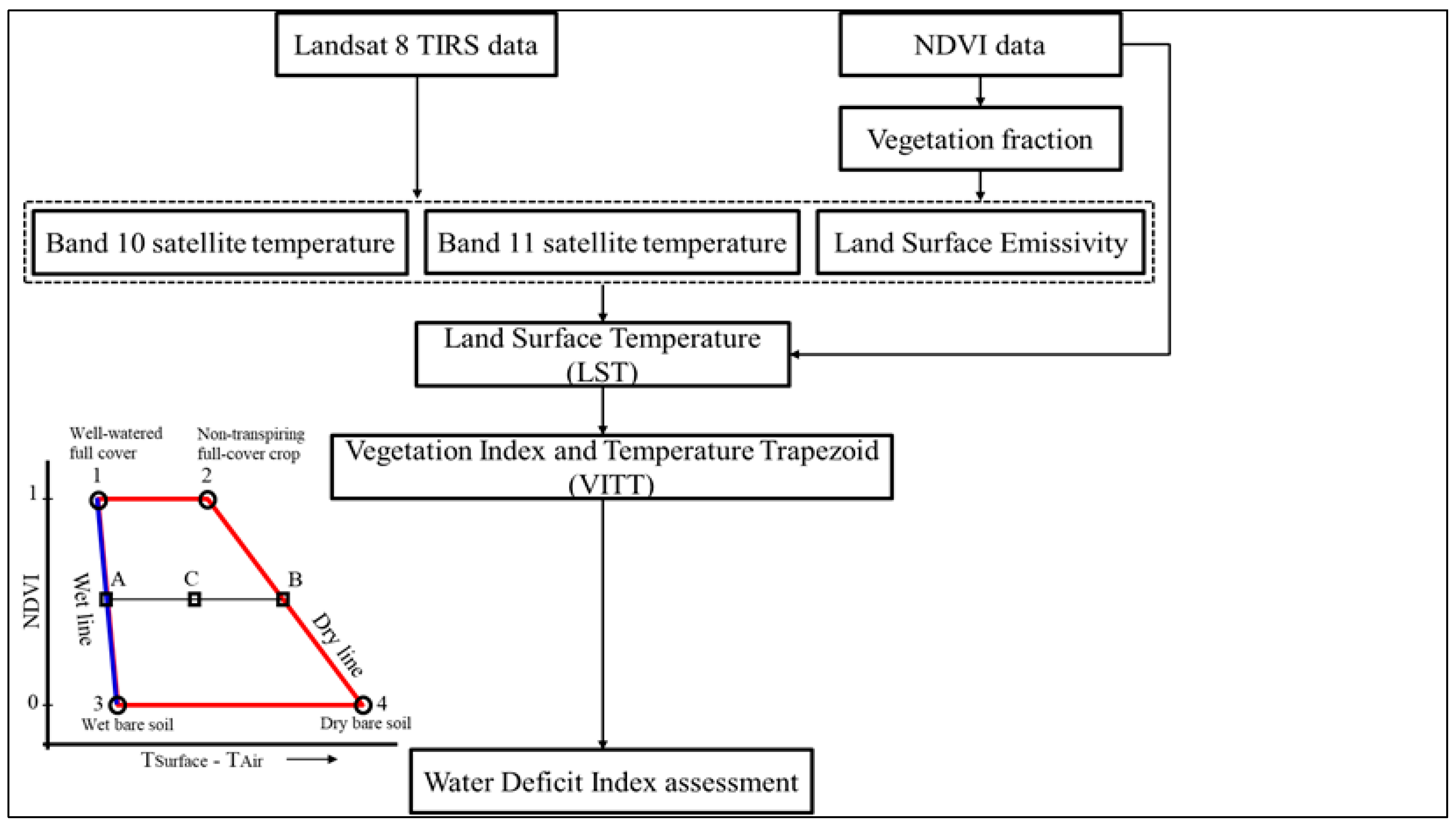
2.3.3. Land Surface Temperature Estimation—WDI Assessment

The methodology adopted for the estimation of Land Surface Temperature (LST) and WDI is synthetized in a flowchart given in Figure 1.
Land surface temperature was retrieved from Landsat 8 thermal infrared sensor bands using the Split Window (SW) algorithm proposed by Jimenez-Munoz and Sobrino [61]:
T s = T 10 + c 1 ( T 10 T 11 ) + c 2 ( T 10 T 11 ) 2 + c 0 + ( c 3 + c 4 w ) ( 1 ε ) + ( c 5 + c 6 w ) ε  
where ε is the mean emissivity ε = 0.5 ( ε i + ε j . ), ε is the emissivity difference ε = ( ε i ε j . ), W is the total atmospheric water vapor content (g/cm²), and c0–c6 are the Split Window coefficients.
Thermal infrared sensor data of both bands (10 and 11) of all the Landsat images were converted into spectral radiance as mentioned above. The retrieved radiance was converted into brightness temperature (TB) using the thermal constants provided in the Landsat metadata.
Brightness temperature (in Kelvin), for each pixel within the extracted region, was applied as follows:
T B = K 2 ln ( K 1 L λ + 1 )
where TB is the at-satellite brightness temperature (K); Lλ is the TOA spectral radiance (W/m²/srad/μm); and K1 and K2 are the band-specific thermal conversion constants (Table 2).
The split-window coefficients c0 to c6 (Table 3) were extracted from simulated data reported by Skokovic et al. [62].
In this study, the land surface temperature retrieval method was used with previously known Land Surface Emissivity (LSE), since the simultaneous methods need specific requirements and sophisticated algorithms, while the previously known land surface emissivity methods appear to be more practical with reasonable accuracy for land surface temperature retrieval from Landsat imagery. Emissivity ( ε ) is estimated following NDVI thresholds method retrieved using Sobrino et al. [63,64] and Wang et al. [65].
ε i = {   a i ρ red + b i   ;   NDVI   < 0.2   ε v , i P v + ε s , i ( 1 P v ) + C i ; 0.2 <   NDVI   < 0.5   ε v , i + C i ;   NDVI   > 0.5
The emissivity of vegetation (εv) and soil (εs) was calculated from the Moderate Resolution Imaging Spectroradiometer (MODIS) UCSB (University of California, Santa Barbara) emissivity library, using the following equation:
ε i = λ 1 , i λ 2 , i f i ( λ ) ε i ( λ ) d λ λ 1 , i λ 2 , i f i ( λ ) d λ
where εi is the emissivity for channel I, εi(λ) is the spectral emissivity, λi is the effective band wavelength for band I, and f i ( λ ) . is the spectral response function for correspondent band.
Soil and vegetation emissivity’s values for Landsat 8 TIRS are reported in Table 4.
The vegetation fraction (Pv) is derived from NDVI [63,66]:
P v = ( NDVI NDVI min NDVI max NDVI min ) 2
where NDVImin = 0.2 and NDVImax = 0.5.
Ci is a term which considers the cavity effect due to the surface roughness (C = 0 for flat surfaces). Sobrino et al. [67] suggested that Ci can be estimated as follows:
C i = ( 1 ε s , i ) ε v , i   F ( 1 P v )
where F′ is the geometrical factor ranging between 0 and 1, depending on the geometrical distribution of the surface (usually 0.55).
When NDVI < 0.2 (never occurred in this experiment), the pixel was considered as bare soil (Pv = 0). For this circumstance, the emissivity was estimated from an empirical relationship with the red band reflectance (R), which is also derived from MODIS UCSB emissivity library [64,68,69]. The relationships for band 10 and 11 were ε 10 = 0.973–0.047 R and ε 11 = 0.984−0.026 R.
Different vegetation indices such as NDVI, MSAVI, and SAVI may have different linkages with land surface temperature providing the design basis of the vegetation index/temperature trapezoid. In this research, the NDVI was utilized since it shows more sensitivity to partial covers in early stages of the crop. The corners of the vegetation index/temperature trapezoid were determined using the measured values of wheat NDVI during several crop stages under conditions of rainfed and full irrigation and the difference between surface and air temperature. For a given pixel, we combined visible, infrared, and thermal datasets. The correlation between three bands has proven to be useful for appropriate monitoring of vegetation and water stress. Then, the vertices were defined and the empirical vegetation index/temperature trapezoid was built. It led to the definition of the WDI.
The WDI is developed to combine the NDVI and land surface temperature data to detect changes in moisture conditions. In this study, the Landsat 8 land surface temperature vs. NDVI relationship in terms of irrigation regimes is interpreted via the vegetation index/temperature trapezoid, which is a simplification of the WDI model.

2.4. Statistical Analysis

Linear regression analysis was applied to assess the relationship between crop physiological and biometric data and vegetation indices, whereas the exponential regression analysis was used to evaluate the relationship between the ground-based and satellite-based vegetation indices. The coefficient of determination (R²) was considered to judge the strength of relationships.
All statistical analyses were carried out using SAS University Edition (Cary, NC, USA).

3. Results and Discussion

3.1. Ground-Based Sensing Results

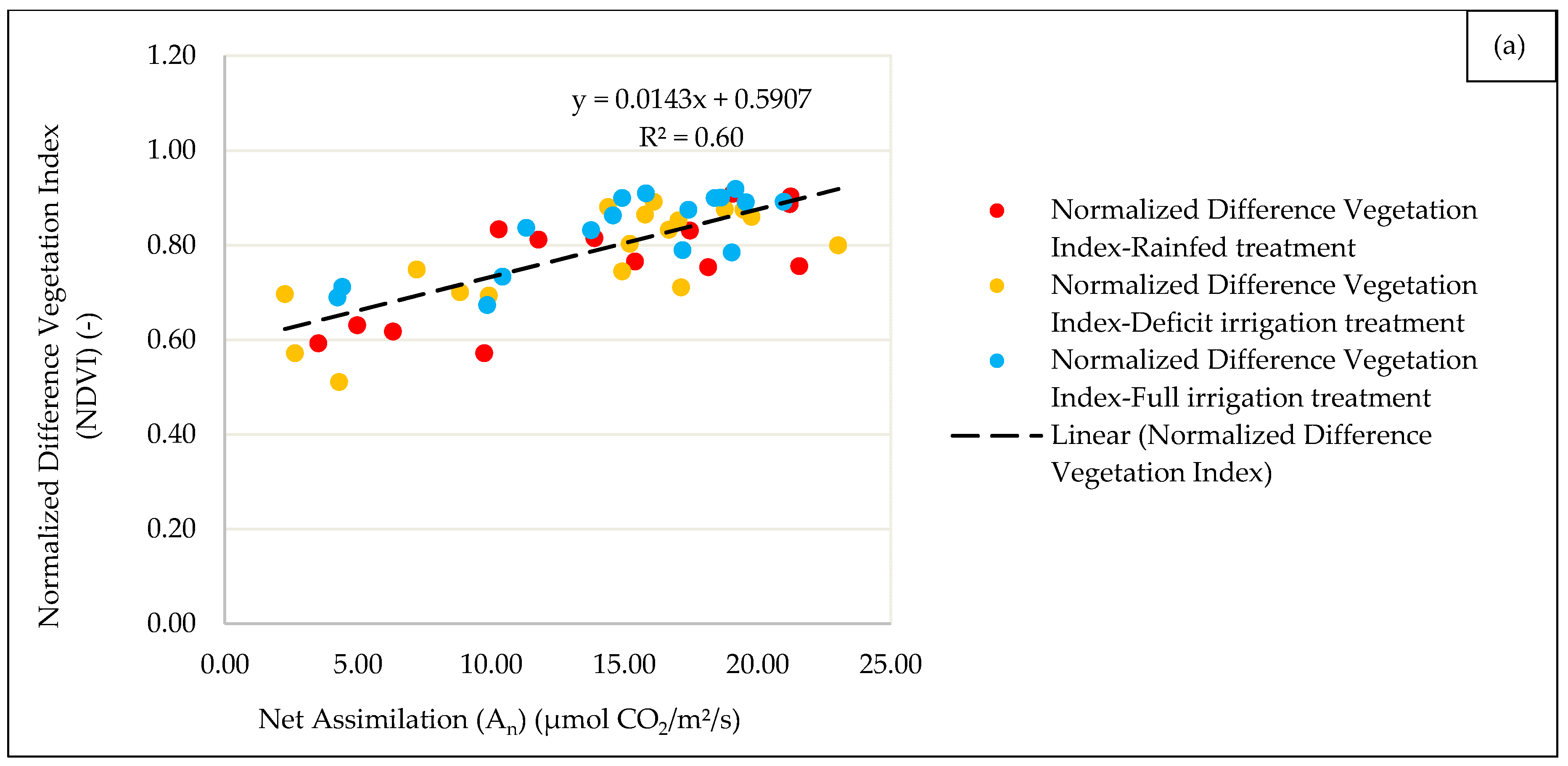
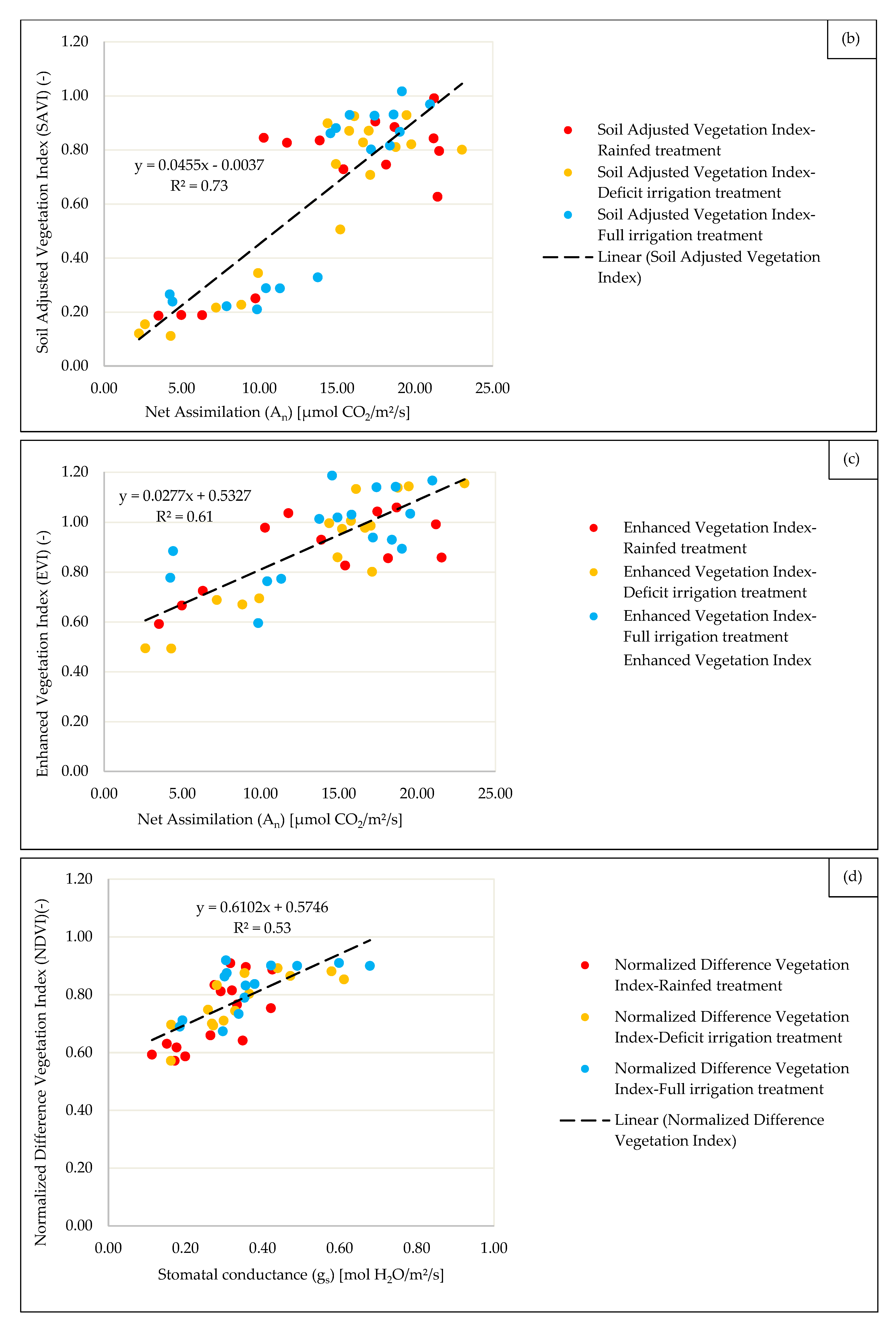
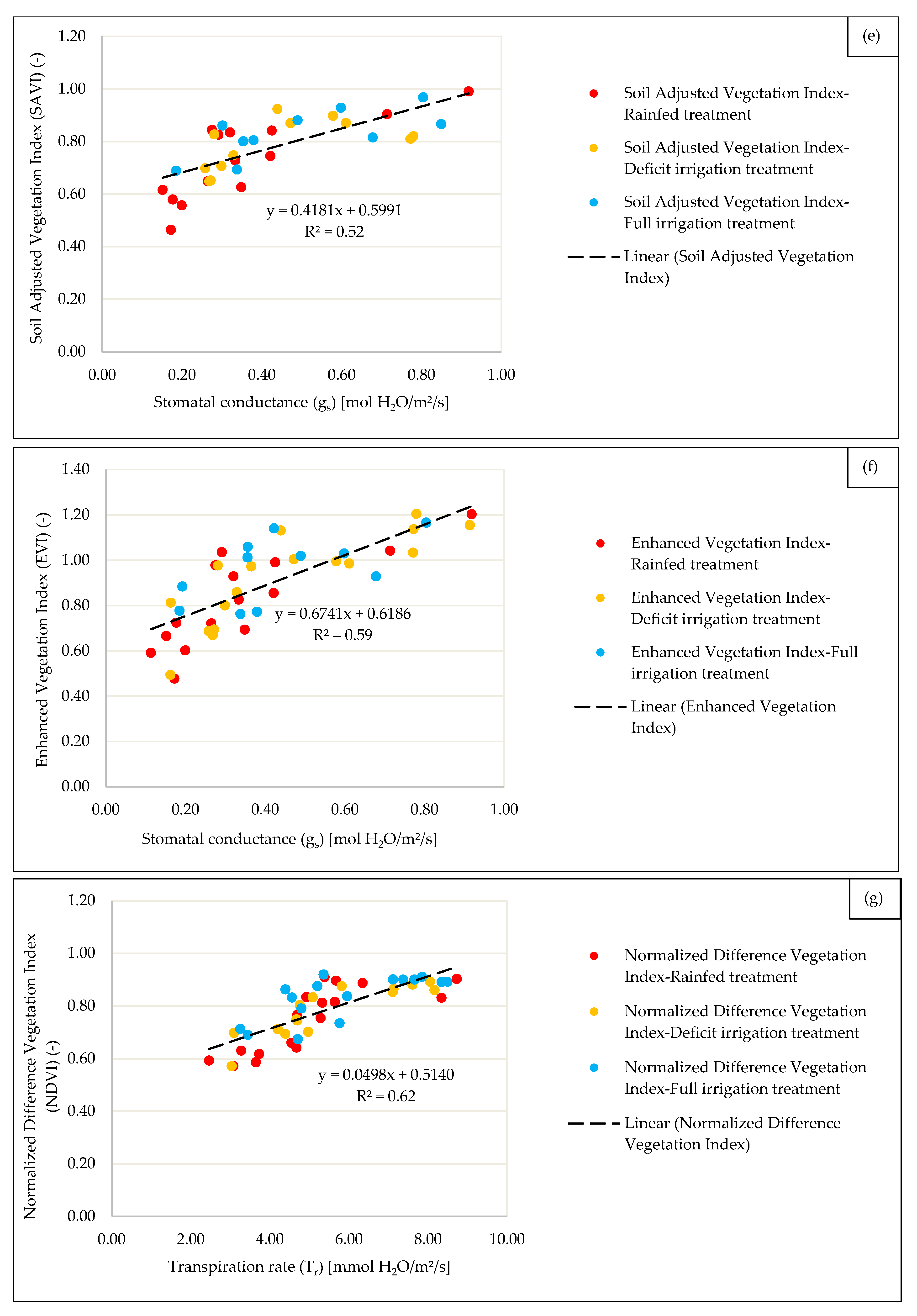
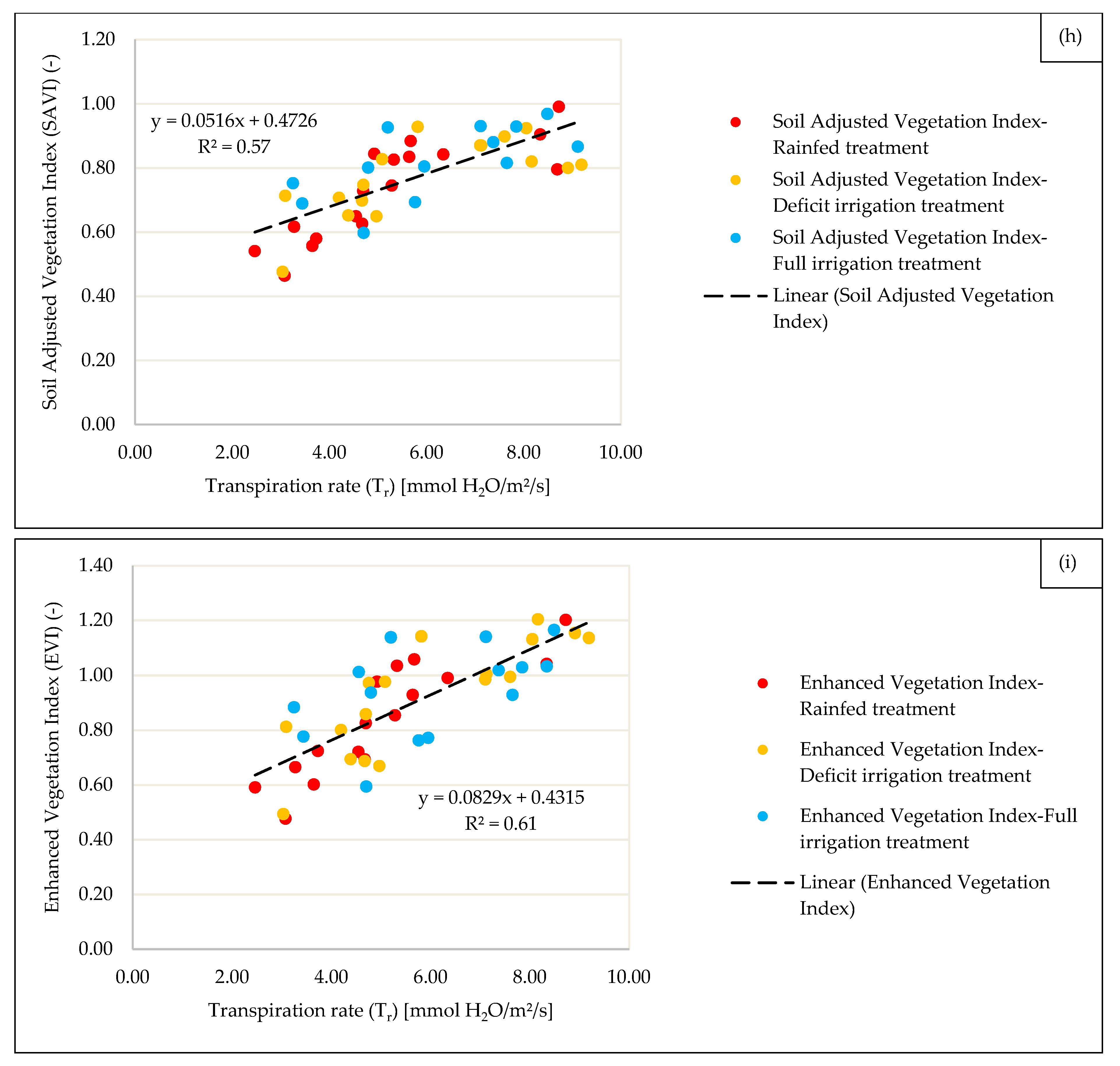
3.1.1. Leaf Gas Exchange Parameters Versus VIs Measured at Canopy Scale

The parameters of the linear regressions linking the measured gas exchange variables (stomatal conductance, net assimilation. and transpiration rate), with thermal (WDI) and spectral (NDVI, SAVI, and EVI) VIs are presented in Figure 2 and Figure 3, respectively. The linear regression function was chosen since it was applied successfully in several other studies [70,71,72,73].
Overall, the optical-based Leaf Gas Exchanges (LGE) models performed consistently well. A positive correlation between leaf gas exchanges and NDVI, SAVI, and EVI was observed. Nevertheless, a negative correlation between leaf gas exchanges and WDI was apparent. The R² of VI-based leaf gas exchange estimation ranged from 0.52 to 0.75. EVI demonstrated slightly better performance than SAVI and NDVI (Figure 3). Under these circumstances, WDI was found to perform strongly with the abovementioned parameters, since surface temperature (Ts) measurements were reliable in determining the four corners of the vegetation index/temperature trapezoid data-range. It was shown that the thermal information had a stronger capacity of estimating leaf gas exchanges than optical data.
The ability of optical-based and thermal-based data to estimate leaf gas exchanges was evaluated. Land surface temperature provided valuable information to quantify surface energy balance, and it is theoretically linked with leaf gas exchanges in the form of WDI [74,75]. NDVI, SAVI, and EVI were the indicators of the trend term, whereas WDI was the indicator describing environmental stress. Zhang [76] and Yang et al. [77] used temperature information to measure the influence of drought stress on stomatal conductance. Therefore, employing thermal information as a vital proxy for drought stress is a good alternative. Overall, the presented results demonstrated that the application of optical VIs to estimate leaf gas exchanges is a promising methodology. In particular, good results were observed when WDI was correlated with stomatal conductance (R2 = 0.93) and other LGE parameters (Figure 2). If the thermal information is missing, single optical VIs is also recommended to quantify leaf gas exchanges.
There is not a clear differentiation of results among different water regimes (Figure 3). It might be explained by the relatively low irrigation amount (1050 and 960 m3/ha in 2015 and 2016, respectively) which was applied mainly at the flowering and yield formation phases. Therefore, there was enough precipitation during the booting and stem elongation phase which impeded the occurrence of water stress during crop vegetative development. Accordingly, the VIs could not be suitable to discern among different water regimes.

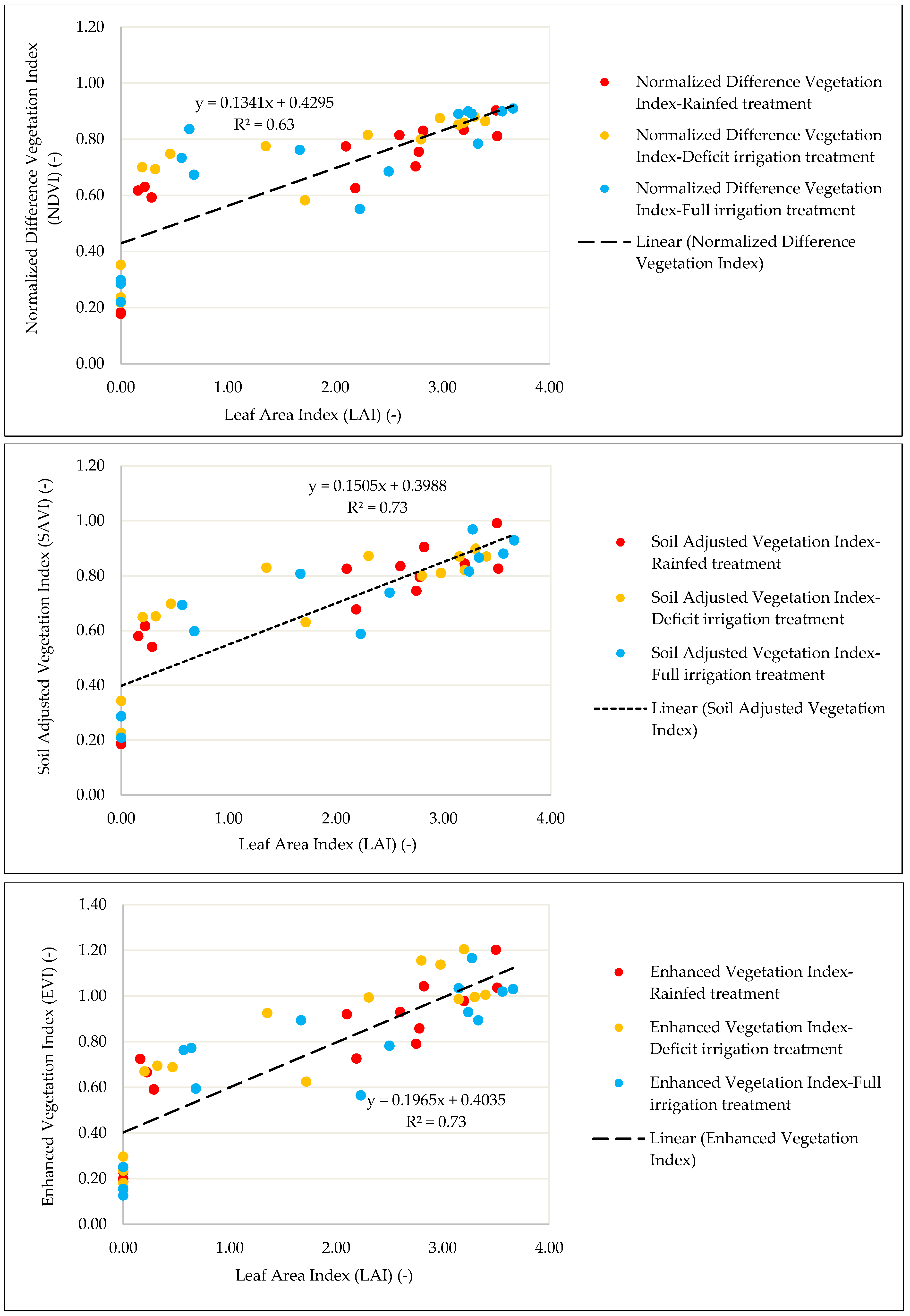
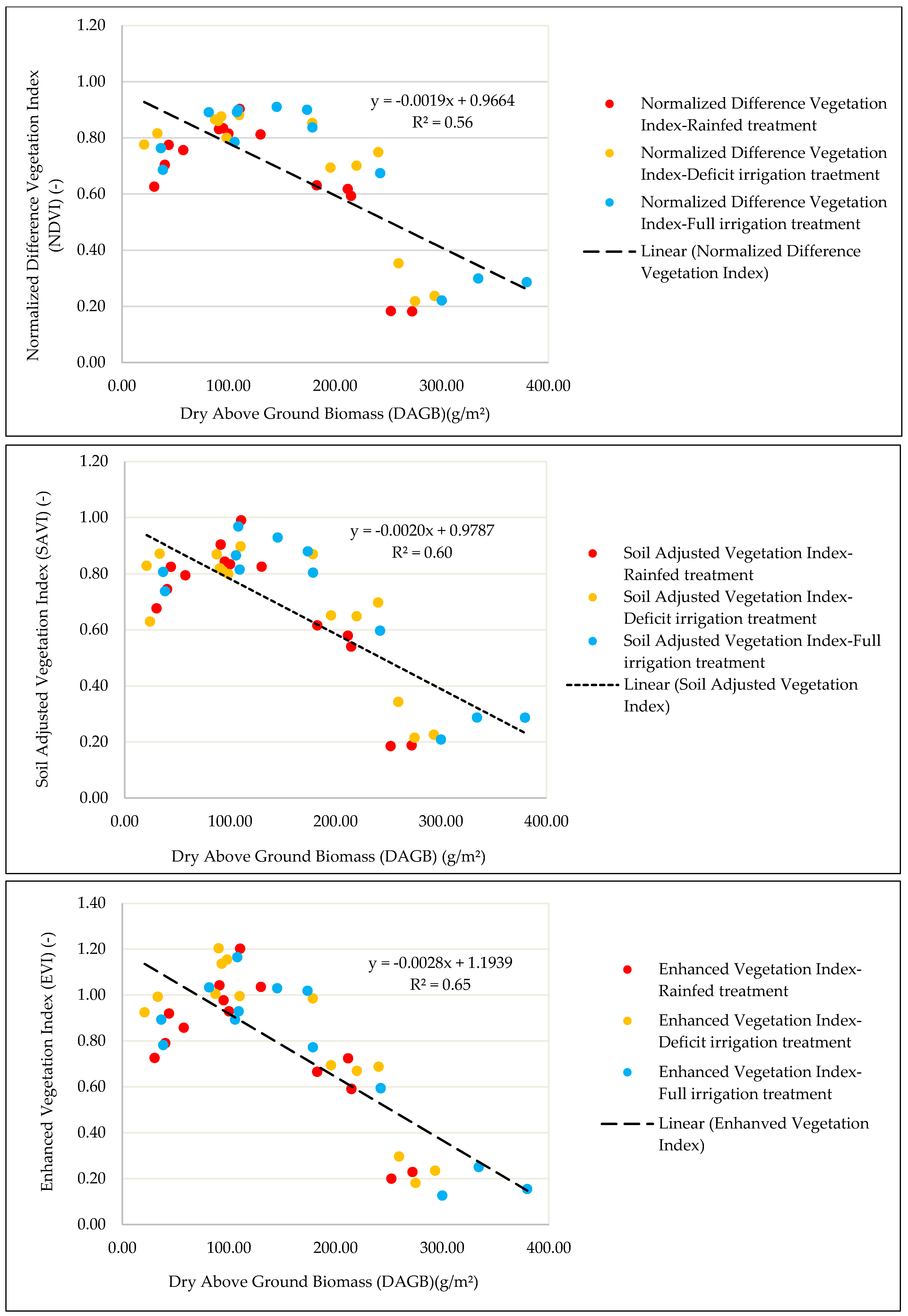
3.1.2. Biometric Crop Parameters Versus VIs Measured at Canopy Scale

The regressions derived from the relationships between canopy scale vegetative indices (i.e., NDVI, SAVI, and EVI) versus biometric crop parameters (leaf area index and dry aboveground biomass) are summarized in Figure 4. A linear regression function was chosen to show the general trend of the above-cited relationships.
The results (Figure 4) indicated that the measured vegetation indices are correlated with LAI to a certain level of agreement. Hence, in the case of LAI, R² ranges between 0.63 (for NDVI) and 0.73 (for both SAVI and EVI).
Up to the initiation of flowering, the averaged LAI increased in all plots, but it started to decrease at the beginning of yield formation and maturity. In this study, both ground-based and satellite mean hyperspectral reflectance of wheat canopy increased at the beginning of the season and then started to decrease, which is consistent with the field measurements of LAI. The present results suggest that LAI can be accurately estimated using spectral vegetation indices. Inasmuch as EVI was significantly affected by soil background, it was strongly correlated with leaf area index (R² = 0.73). This result is in agreement with Fensholt et al. [78], who reported similar findings on grassland.
The results of regression analysis between winter wheat biomass and spectral vegetative indices showed that all measured vegetation indices are correlated with biomass to a certain level of agreement (Figure 4). The correlation of Dry Aboveground Biomass (DAGB) was better with EVI (R² = 0.65) than with SAVI (R2 = 0.60) and with NDVI (R2 = 0.56).
Previous studies have shown that near infrared and red band vegetation indices are effective for estimating DAGB [79,80,81]. Nevertheless, in this research, the correlation between DAGB, and red and near infrared band vegetation indices is not particularly strong. This can be explained by the fact that, during the reproductive stage, photosynthesis and near infrared reflectance both clearly decrease. This result is consistent with the results of Humbeck et al. [82]. Sun et al. [83] reported that, during the middle and late stages of crop growth, wheat reproductive growth was enhanced when the vegetative growth was weakened [84] and that, consequently, the winter wheat Dry Aboveground Biomass (DAGB) continued to increase. However, the chlorophyll content of winter wheat leaves decreased, leading to a decrease in the near infrared reflectance. The relation between near infrared spectral reflectance and crop biomass was then decreased because of the incoming senescence.
Yue et al. [85] reported that red-, green-, and blue-band spectral indices are effective in estimating Dry Aboveground Biomass (DAGB) of winter wheat during vegetative growth and reproductive growth stages.

3.2. Satellite Sensing Results

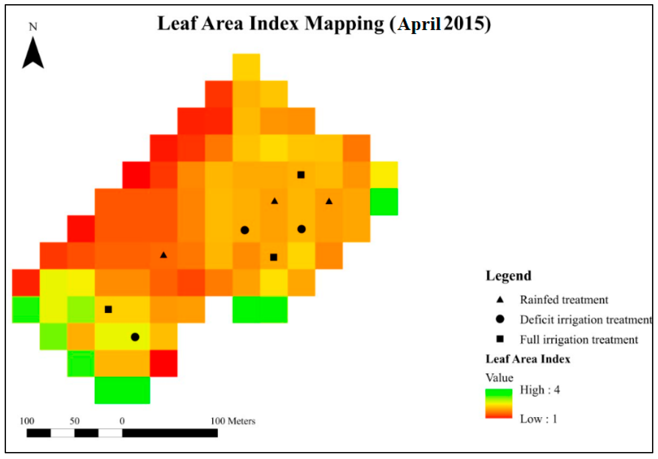
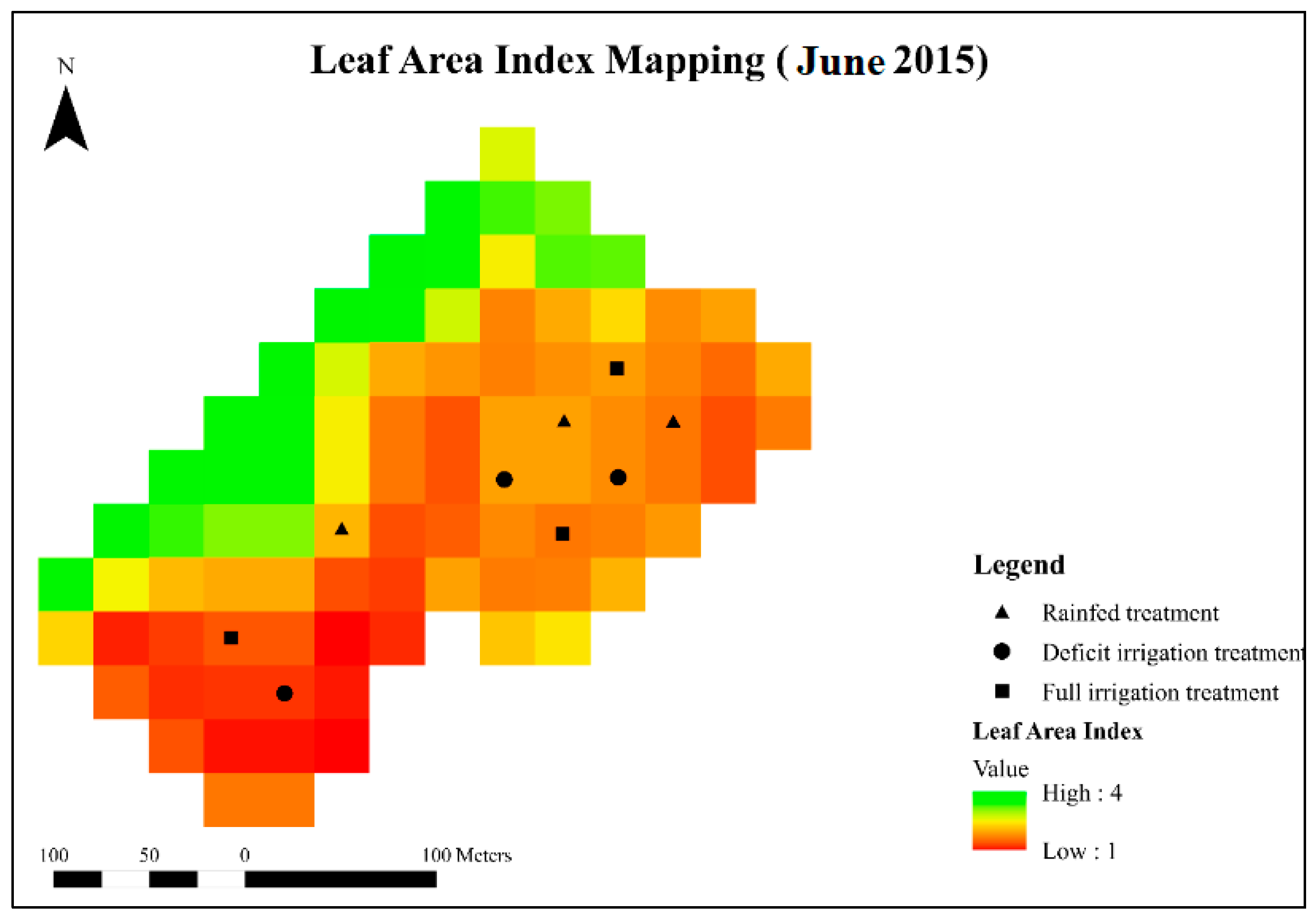
Mapping Leaf Area Index

The LAI maps are shown in Figure 5 for two days (around flowering and maturity) in the first agricultural year. For 16 April 2015, the satellite-based LAI data showed that the LAI was high in all plots. However, the LAI decreased near maturation (03 June 2015). These results are consistent with field observations and data reported by Yue et al. [85].

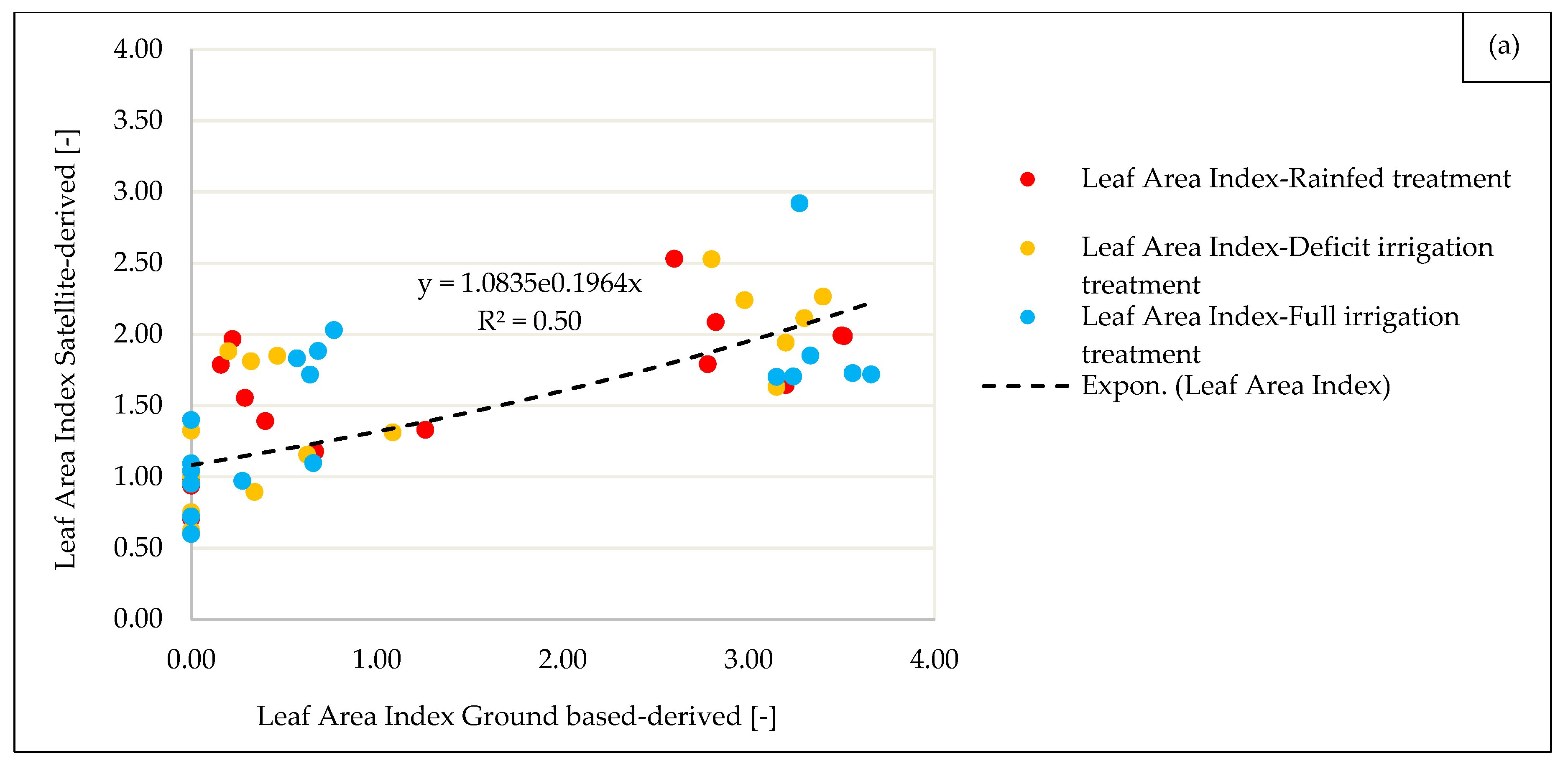
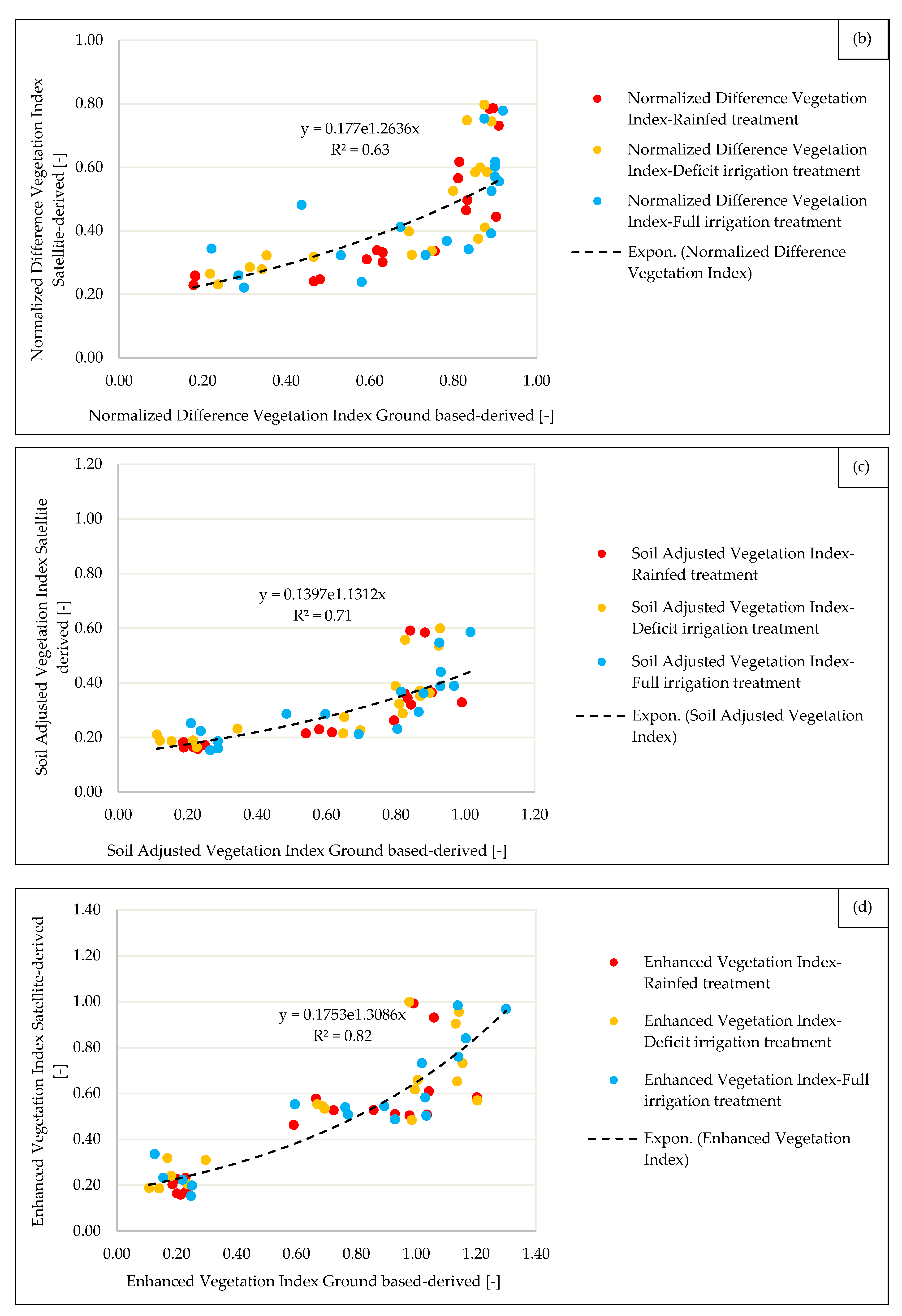
3.3. Satellite vs. Ground-Based VIs Comparison

The type of relationships between LAI, NDVI, SAVI, and EVI measured from satellite and the same parameters measured from ground-based sensing method are given in Figure 6 for both years.
The exponential regression function was chosen to show the general trend of the LAI, NDVI, SAVI, and EVI VIs. High correlations appeared to be evident for LAI, NDVI, SAVI, and EVI regressions, with R² values close to or higher than 0.70. The highest determination coefficient (R² = 0.83) was obtained in the case of EVI. Again, there is no clear differentiation among different water regimes due to the facts explained previously in Section 3.1.1.
Biudes et al. [86] reported that LAI estimated on ground-based and satellite-derived extinction were positively correlated with crop growth. The NDVI correlation was relatively high, in agreement with other studies [87,88,89].
This study has confirmed the applicability of both ground-based and satellite remote sensing techniques to evaluate crop growth and plant physiological parameters of winter wheat. The VIs obtained on the ground-based measurements performed slightly better than those acquired by the satellite sensors.
Landsat and Sentinel 2 remote sensing data could be particularly useful for the regional assessments and field crops grown on large plots since these data cover greater areas and are available free of charge. Inasmuch as the limitations are related to the spatial resolution and revisiting frequency, the Landsat data offered a valuable input to assess winter wheat biometric and physiological parameters. Moreover, Landsat and Sentinel 2 data can be used in a complementary way. The limitation of use of satellite data under cloud conditions does not represent a serious drawback in the arid and semiarid areas of the Mediterranean region despite the cloud presence and precipitation. Therefore, the availability of Landsat and Sentinel 2 data provides the opportunity to develop specific operational tools, based on the historical earth observation sensing data and wheat management practices on the ground, to analyze the pros and cons of adopted agronomic practices in the past and to identify the best crop management for the future. Although a new generation of satellites with improved spatial resolution and reduced return frequency is available, the use of Landsat data remains essential due to the longest continuously running global data archive and the possibility to analyze the crop performance for a long period in the past.
Figure 7 shows the VIT trapezoid formed for winter wheat from ground-based and satellite data obtained for the first experimental year (2014–2015). The circles within the trapezoid correspond to measurements of (Ts − TA) and NDVI from the area planted with wheat. Both sensing methods were used to verify that all samples fell within the limits of the empirical trapezoid. The data showed either high or low values of NDVI and (Ts − TA); some intermediate values were also recorded.
The surface temperature values, measured to define the trapezoidal method for winter wheat, agree with those reported by Jackson [90], Moran et al. [47], and Mendez-Barroso et al. [91]. They mentioned that the temperature of dry bare soil is always several degrees above the air temperature, generally by more than 10–15 °C, because the soil thermal inertia is relatively low [92] and soil moisture is one of the factors affecting the thermal properties of the soil.
The empirical trapezoid model proposed in this study can be a useful tool to estimate the spatial and temporal extent of WDI, which is applied to identify the degree of water stress. The development of this remote sensing method is a priority in arid and semiarid zones where water is a scarce resource. Moreover, it requires a reduced number of inputs, which are relatively easy to obtain, such as NDVI, air, and surface temperatures. Generally, WDI produced a good estimation of surface temperature and, thus, evapotranspiration because it was able to capture the growth process of leaves and to describe the temporal variation trend of stomatal conductance.

4. Conclusions

In this study, ground-based and satellite remote sensing techniques were used to evaluate and to compare crop growth and crop water status of winter wheat under three water regimes. The results of elaborations of data from two growing seasons indicated the following:
  • A strong correlation between the spectral vegetative indices (NDVI, SAVI, and EVI) and LAI at the canopy scale. However, the relationship with dry aboveground biomass was less convincing. As related to leaf gas exchange parameters, WDI responded well to the increasing level of water stress. Data in the thermal infrared spectrum were the most promising source to monitor water stress, showing better correlations than the spectral vegetative indices.
  • Despite the challenges posed by moderate satellite spatial resolution, the correlations between the satellite and ground-based results were satisfactory and consistent with other studies.
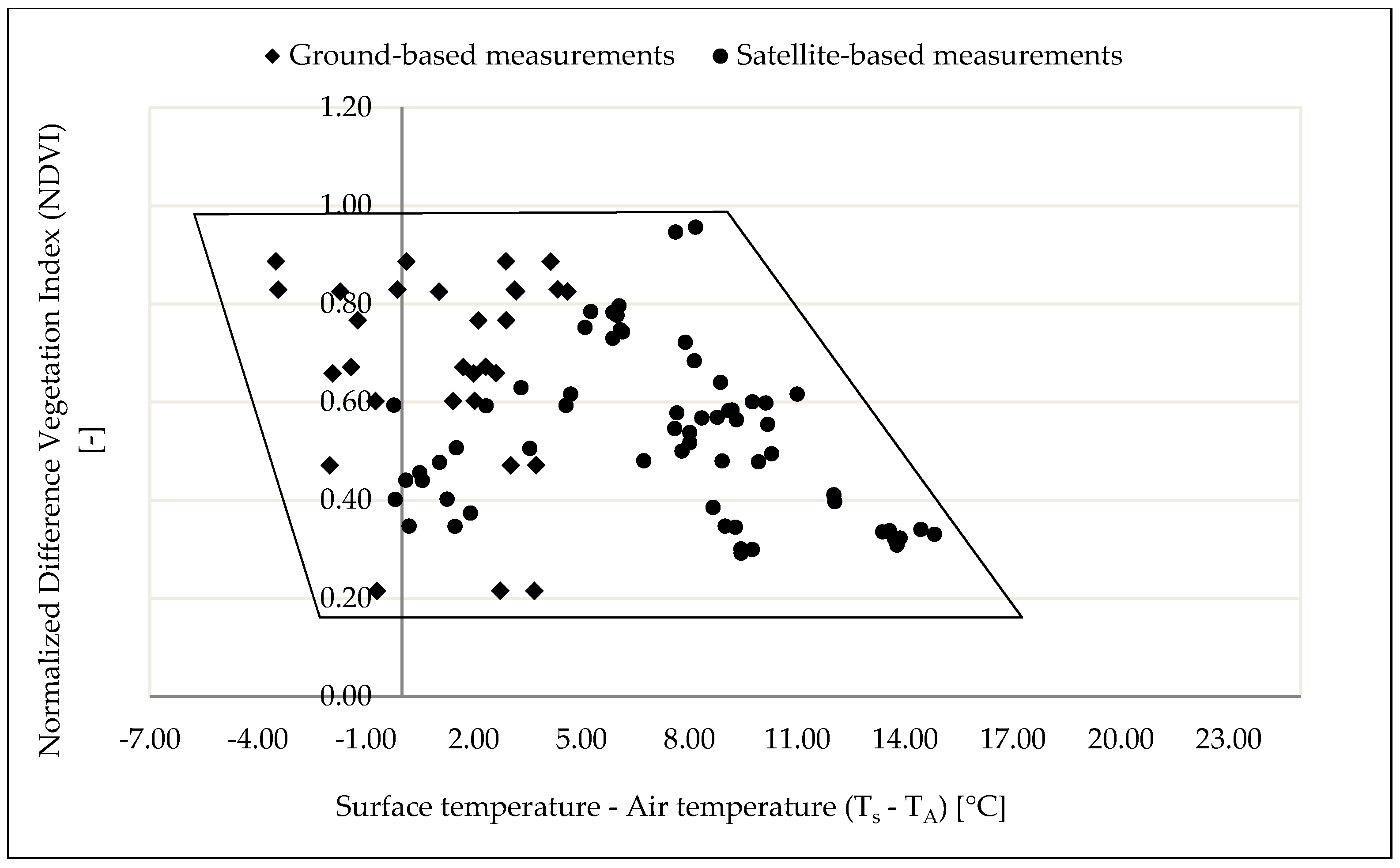
  • The Vegetation Index/Temperature (VIT) trapezoid concept, based on Landsat 8 thermal bands and surface temperature data, constitutes a relevant approach to estimate the spatial and temporal extent of water stress. Nevertheless, it is more suitable for summer than for winter–spring crops.
Agricultural sector requires continuous monitoring systems able to provide timely data on crop growth, water/nutrient/health status, and biomass/yield in a standardized and regular manner at different scales (farm, regional, and national). The estimates should be provided as early as possible during the growing season(s), compared with the previous seasons, and updated periodically throughout the season until harvesting. The availability of remote sensing data should enable the agricultural engineers and water managers to identify the areas with the large variation of crop biometric and physiological parameters and to make adequate management decisions in order to stabilize and to improve yield and water productivity.

Author Contributions

Conceptualization, V.C., R.A. and M.T.; methodology, N.M., G.D.M. and M.T.; experimental measurements, N.M.; software, N.M.; formal analysis, N.M. and S.M.H.; writing—original draft preparation, N.M.; writing—review and editing, N.M., V.C., R.A. and M.T.; supervision, V.C., R.A. and M.T. All authors have read and agreed to the published version of the manuscript.

Funding

This research was carried out under the Master of Science Program on “Sustainable water and land management in Mediterranean agriculture” funded by CIHEAM - Mediterranean Institute of Bari.

Acknowledgments

The research was supported by the Master of Science Program in Land and Water Resources Management of CIHEAM-IAMB (Bari, Italy). The authors thank Carlo Ranieri, Domenico Tribuzio and Mohamed Ben Brahim (CIHEAM-IAMB) for technical support during the acquisition of data and Giovanni Manolio (experimental farm “E. Pantanelli”) for agronomic assistance in the field.

Conflicts of Interest

The authors declare no conflict of interest.

References

  1. Liu, P. A survey of remote-sensing big data. Front. Environ. Sci. 2015, 3, 1–6. [Google Scholar] [CrossRef] [Green Version]
  2. Chi, M.; Plaza, A.; Benediktsson, J.A.; Sun, Z.; Shen, J.; Zhu, Y. Big data for remote sensing: Challenges and opportunities. Proc. IEEE 2016, 104, 2207–2219. [Google Scholar] [CrossRef]
  3. Khanal, S.; John, F.; Scott, S. An overview of current and potential applications of thermal remote sensing in precision agriculture. Comput. Electron. Agric. 2017, 139, 22–32. [Google Scholar] [CrossRef]
  4. Huang, Y.; Zhong-Xin, C.; Tao, Y.; Xiang-Zhi, H.; Xing-Fa, G. Agricultural remote sensing big data: Management and applications. J. Integr. Agric. 2018, 17, 1915–1931. [Google Scholar] [CrossRef]
  5. Gebbers, R.; Adamchuk, V.I. Precision agriculture and food security. Science 2010, 327, 828–831. [Google Scholar] [CrossRef] [PubMed]
  6. Jovanovic, N.; Pereira, L.S.; Paredes, P.; Pôças, I.; Cantore, V.; Todorovic, M. A review of strategies, methods and technologies to reduce non-beneficial consumptive water use on farms considering the FAO56 methods. Agric. Water Manag. 2020, 239, 106267. [Google Scholar] [CrossRef]
  7. Sakamoto, T.; Gitelson, A.A.; Arkebauer, T.J. MODIS-based corn grain yield estimation model incorporating crop phenology information. Remote Sens. Environ. 2013, 131, 215–231. [Google Scholar] [CrossRef]
  8. Solano, R.; Didan, K.; Jacobson, A.; Huete, A. MODIS Vegetation Index User’s Guide (MOD13 Series). In Vegetation Index and Phenology Lab, 2nd ed.; The University of Arizona: Tucson, AZ, USA, 2010. [Google Scholar]
  9. Bulcock, H.H.; Jewitt, G.P.W. Spatial mapping of leaf area index using hyperspectral remote sensing for hydrological applications with a particular focus on canopy interception. Hydrol. Earth Syst. Sci. 2010, 14, 383–392. [Google Scholar] [CrossRef] [Green Version]
  10. Chéret, V.; Denux, J.P. Analysis of Modis NDVI time series to calculate indicators of Mediterranean forest fire susceptibility. Gisci. Remote Sens. 2011, 48, 171–194. [Google Scholar] [CrossRef]
  11. Sims, N.C.; Colloff, M.J. Remote sensing of vegetation responses to flooding of a semi-arid floodplain: Implications for monitoring ecological effects of environmental flows. Ecol. Indic. 2012, 18, 387–391. [Google Scholar] [CrossRef]
  12. Johansen, B.; Tommervik, H. The Relationship between Phyto-mass, NDVI and Vegetation Communities Svalbard. Int. J. Appl. Earth Obs. Geoinf. 2014, 27, 20–30. [Google Scholar] [CrossRef]
  13. Eckert, S.; Hüsler, F.; Liniger, H.; Hodel, E. Trend analysis of MODIS NDVI time series for detecting land degradation and regeneration in Mongolia. J. Arid Environ. 2015, 113, 16–28. [Google Scholar] [CrossRef]
  14. Basso, B.; Cammarano, D.; De Vita, P. Remotely sensed vegetation indices: Theory and applications for crop management. Rivista Italiana Di Agrometeorologia 2004, 1, 36–53. [Google Scholar]
  15. Panda, S.S.; Ames, D.P.; Panigrahi, P. Application of Vegetation Indices for Agricultural Crop Yield Prediction Using Neural Network Techniques. J. Remote Sens. 2010, 2, 673–696. [Google Scholar] [CrossRef] [Green Version]
  16. Allbed, A.; Kumar, L.; Aldakheel, Y.Y. Assessing soil salinity using soil salinity and vegetation indices derived from IKONOS high-spatial resolution imageries: Applications in a date palm dominated region. Geoderma 2014, 230–231, 1–8. [Google Scholar] [CrossRef]
  17. Veraverbeke, S.; Gitas, I.; Katagis, T.; Polychronaki, A.; Somers, B.; Goossens, R. Assessing post-fire vegetation recovery using red-near infrared vegetation indices: Accounting for background and vegetation variability. ISPRS J. Photogramm. Remote Sens. 2012, 68, 28–39. [Google Scholar] [CrossRef] [Green Version]
  18. Zhang, X.Y.; Friedl, M.A.; Schaaf, C.B.; Strahler, A.H.; Hodges, J.C.F.; Gao, F.; Reed, B.C.; Huete, A. Monitoring vegetation phenology using MODIS. Remote Sens. Environ. 2003, 84, 471–475. [Google Scholar] [CrossRef]
  19. Huete, A.; Didan, K.; Miura, T.; Rodriguez, E.P.; Gao, X.; Ferreira, L.G. Overview of the radiometric and biophysical performance of the MODIS vegetation indices. Remote Sens. Environ. 2002, 83, 195–213. [Google Scholar] [CrossRef]
  20. Barrett, E.C.; Curtis, L.F. Introduction to environmental remote sensing. In Introduction to Environmental Remote Sensing, 3rd ed.; Barrett, E.C., Curtis, L.F., Eds.; Chapman & Hall: London, UK, 1992. [Google Scholar]
  21. Myneni, R.B.; Hoffman, S.; Knyazikhin, Y.; Privette, J.L.; Glassy, J.; Tian, Y.; Wang, Y.; Song, X.; Zhang, Y.; Smith, G.R.; et al. Global products of vegetation leaf area and fraction absorbed PAR from year one of MODIS data. Remote Sens. Environ. 2002, 83, 214–231. [Google Scholar] [CrossRef] [Green Version]
  22. Cao, R.Y.; Shen, M.G.; Zhou, J.; Chen, J. Modeling vegetation green-up dates across the Tibetan Plateau by including both seasonal and daily temperature and precipitation. Agric. For. Meteorol. 2018, 249, 176–186. [Google Scholar] [CrossRef]
  23. Zhang, X.; Tarpley, D.; Sullivan, J. Diverse responses of vegetation phenology to a warming climate. Geophys. Res. Lett. 2007, 34, 255–268. [Google Scholar] [CrossRef]
  24. Friedl, M.A.; McIver, D.K.; Hodges, J.C.; Zhang, X.Y.; Muchoney, D.; Strahler, A.H.; Woodcock, C.E.; Gopal, S.; Schneider, A.; Cooper, A.; et al. Global land cover mapping from MODIS: Algorithms and early results. Remote Sens. Environ. 2002, 83, 287–302. [Google Scholar] [CrossRef]
  25. Crow, W.T.; Kumar, S.V.; Bolten, J.D. On the utility of land surface models for agricultural drought monitoring. Hydrol. Earth Syst. Sci. 2012, 16, 3451–3460. [Google Scholar] [CrossRef] [Green Version]
  26. Huete, A. A soil-adjusted vegetation index (SAVI). Remote Sens. Environ. 1988, 17, 37–53. [Google Scholar] [CrossRef]
  27. Gilbert, M.A.; Gonzalez-Piqueras, J.; Garcıa-Haro, F.; Melia, J. A generalized soil-adjusted vegetation index. Remote Sens. Environ. 2002, 82, 303–310. [Google Scholar] [CrossRef]
  28. Huete, A.; Justice, C.; Liu, H. Development of vegetation and soil indices for MODIS-EOS. Remote Sens. Environ. 1994, 49, 224–234. [Google Scholar] [CrossRef]
  29. Baret, F.; Guyot, G. Potentials and limits of vegetation indices for LAI and APAR assessment. Remote Sens. Environ. 1991, 35, 161–173. [Google Scholar] [CrossRef]
  30. Qi, J.; Chehbouni, A.; Huete, A.R.; Kerr, Y.H. Modified Soil Adjusted Vegetation Index (MSAVI). Remote Sens. Environ. 1994, 48, 119–126. [Google Scholar] [CrossRef]
  31. Rondeaux, G.; Steven, M.; Baret, F. Optimization of soil-adjusted vegetation indices. Remote Sens. Environ. 1996, 55, 95–107. [Google Scholar] [CrossRef]
  32. Liu, H.Q.; Huete, A. A feedback-based modification of the NDVI to minimize canopy background and atmospheric noise. IEEE Trans. Geosci. Remote Sens. 1995, 33, 457–465. [Google Scholar] [CrossRef]
  33. Huete, A.; Justice, C. MODIS Vegetation Index (MOD 13) Algorithm Theoretical Basis Document. Am. J. Plant Sci. 1999, 7, 1–59. [Google Scholar]
  34. Weng, Q. Thermal infrared remote sensing for urban climate and environmental studies: Methods, applications, and trends. Remote Sens. 2009, 64, 335–344. [Google Scholar] [CrossRef]
  35. Stark, B.; Smith, B.; Chen, Y. Survey of thermal infrared remote sensing for Unmanned Aerial Systems. In International Conference on Unmanned Aircraft Systems (ICUAS); IEEE: Orlando, FL, USA, 2014; pp. 1294–1299. [Google Scholar]
  36. Anderson, M.C.; Hain, C.; Otkin, J.; Zhan, X.; Mo, K.; Svoboda, M.; Wardlow, B.; Pimstein, A. An Intercomparison of Drought Indicators Based on Thermal Remote Sensing and NLDAS-2 Simulations with U.S. Drought Monitor Classifications. J. Hydrometeorol. 2013, 14, 1035–1056. [Google Scholar] [CrossRef]
  37. Gago, J.; Douthe, C.; Coopman, R.E.; Gallego, P.P.; Ribas-Carbo, M.; Flexas, J.; Escalona, J.; Medrano, H. UAVs challenge to assess water stress for sustainable agriculture. Agric. Water Manag. 2015, 153, 9–19. [Google Scholar] [CrossRef]
  38. Radoglou-Grammatikis, P.; Sarigiannidis, P.; Lagkas, T.; Moscholios, I. A compilation of UAV applications for precision agriculture. Comput. Netw. 2020, 72, 107148. [Google Scholar] [CrossRef]
  39. Calderón, R.; Navas-Cortés, J.A.; Lucena, C.; Zarco-Tejada, P.J. High-resolution airborne hyperspectral and thermal imagery for early detection of Verticillium wilt of olive using fluorescence, temperature and narrow-band spectral indices. Remote Sens. Environ. 2013, 139, 231–245. [Google Scholar] [CrossRef]
  40. Sagan, V.; Maimaitijiang, M.; Sidike, P.; Eblimit, K.; Peterson, K.; Hartling, S.; Esposito, F.; Khanal, K.; Newcomb, M.; Pauli, D.; et al. UAV-Based High Resolution Thermal Imaging for Vegetation Monitoring, and Plant Phenotyping Using ICI 8640 P, FLIR Vue Pro R 640, and thermoMap Cameras. Remote Sens. 2019, 11, 330. [Google Scholar] [CrossRef] [Green Version]
  41. Ludovisi, R.; Tauro, F.; Salvati, R.; Khoury, S.; Mugnozza, G.S.; Harfouche, A. Uav-based thermal imaging for high-throughput field phenotyping of black poplar response to drought. Front. Plant Sci. 2017, 8, 1–18. [Google Scholar] [CrossRef]
  42. Costa, J.M.; Grant, O.M.; Chaves, M.M. Thermography to explore plant-environment interactions. J. Exp. Bot. 2013, 64, 3937–3949. [Google Scholar] [CrossRef]
  43. Ghulam, A.; Li, Z.L.; Qin, Q.; Yimit, H.; Wang, J. Estimating crop water stress with ETM+ NIR and SWIR data. Agric. For. Meteorol. 2008, 148, 1679–1695. [Google Scholar] [CrossRef]
  44. Alves, I.; Pereira, L.S. Non-water-stressed baselines for irrigation scheduling with infrared thermometers: A new approach. Irrig. Sci. 2000, 19, 101–106. [Google Scholar] [CrossRef]
  45. Jones, H.G.; Stoll, M.; Santos, T.; De Sousa, C.; Chaves, M.M.; Grant, O.M. Use of infrared thermography for monitoring stomatal closure in the field: Application to grapevine. J. Exp. Bot. 2002, 53, 2249–2260. [Google Scholar] [CrossRef] [PubMed]
  46. Leinonen, I.; Jones, H.G. Combining thermal and visible imagery for estimating canopy temperature and identifying plant stress. J. Exp. Bot. 2004, 55, 1423–1431. [Google Scholar] [CrossRef] [PubMed] [Green Version]
  47. Moran, M.S.; Clarke, T.R.; Inoue, Y.; Vidal, A. Estimating crop water deficit using the relation between surface-air temperature and spectral vegetation index. Remote Sens. Environ. 1994, 49, 246–263. [Google Scholar] [CrossRef]
  48. Verhoelst, T.; Granville, J.; Hendrick, F.; Kohler, U.; Lerot, C.; Pommereau, J.P.; Redondas, A.; Van Roozendael, M.; Lambert, J.C. Metrology of ground-based satellite validation: Co-location mismatch and smoothing issues of total ozone comparisons. Atmos. Meas. Tech. 2015, 8, 5039–5062. [Google Scholar] [CrossRef] [Green Version]
  49. Rahman, H. Satellite based crop monitoring and estimation system for food security application in Bangladesh. In Expert Meeting on Crop Monitoring for Improved Food Security; Geography: Vientiane, Laos, 2014. [Google Scholar]
  50. Zhang, J. Multisource remote sensing data fusion: Status and trends. Int. J. Image Data Fusion 2010, 1, 5–24. [Google Scholar] [CrossRef] [Green Version]
  51. Dube, T.; Mutanga, O. Evaluating the utility of the medium-spatial resolution Landsat 8 multispectral sensor in quantifying aboveground biomass in uMgeni catchment, South Africa. ISPRS J. Photogramm. Remote Sens. 2015, 101, 36–46. [Google Scholar] [CrossRef]
  52. Roy, D.P.; Qin, Y.; Kovalskyy, V.; Vermote, E.F.; Ju, J.; Egorov, A.; Hansen, M.C.; Kommareddy, I.; Yan, L. Conterminous United States demonstration and characterization of MODIS-based Landsat ETM + atmospheric correction. Remote Sens. Environ. 2014, 140, 433–449. [Google Scholar] [CrossRef] [Green Version]
  53. Wulder, M.A.; Hilker, T.; White, J.C.; Coops, N.C.; Masek, J.G.; Pflugmacher, D.; Crevier, Y. Virtual constellations for global terrestrial monitoring. Remote Sens. Environ. 2015, 170, 62–76. [Google Scholar] [CrossRef] [Green Version]
  54. Cantore, V.; Iovino, F.; Pontecorvo, G. Aspetti Climatici e Zone Fitoclimatiche Della Basilicata; CNR-IEIF: Cosenza, Italy, 1987; p. 49. [Google Scholar]
  55. Cassi, F.; Viviano, L. Suoli della Basilicata—Carta pedologica della Regione Basilicata in scala 1:250.000. In Regione Basilicata—Dip. Agricoltura e Sviluppo Rurale. Direzione Generale; Reg. Basilicata-Dip. Agric. Svilup. Rurale. Dir. Gen.: Potenza, Italy, 2006. [Google Scholar]
  56. Allen, R.G.; Pereira, L.S.; Raes, D.; Smith, M. Crop evapotranspiration. In FAO Irrigation and Drainage Paper 56; FAO: Rome, Italy, 1998; p. 300. [Google Scholar]
  57. Todorovic, M. An Excel-based tool for real time irrigation management at field scale. In Proceedings of the International Symposium on Water and Land Management for Sustainable Irrigated Agriculture, Adana, Turkey, 4–8 April 2006. [Google Scholar]
  58. Li, J.; Roy, D.P. A global analysis of Sentinel-2A, Sentinel-2B and Landsat-8 data revisit intervals and implications for terrestrial monitoring. Remote Sens. 2017, 9, 902. [Google Scholar]
  59. Rouse, J.W.; Haas, R.H.; Schell, J.A.; Deering, D.; Deering, W. Monitoring vegetation systems in the Great Plains with ERTS. In Proceedings of the ERTS Third Symposium, NASA SP-351, Washington, DC, USA, 10–14 December 1973; pp. 309–317. [Google Scholar]
  60. Boegh, E.; Soegaard, H.; Thomsen, A. Evaluating evapotranspiration rates and surface conditions usig Landsat TM to estimate atmospheric resistance and surface resistance. Remote Sens. Environ. 2002, 79, 329–343. [Google Scholar] [CrossRef]
  61. Jimenez-Munoz, J.C.; Sobrino, J.A. Split-Window Coefficients for Land Surface Temperature Retrieval from Low-Resolution Thermal Infrared Sensors. IEEE Geosci. Remote Sens. Lett. 2008, 5, 806–809. [Google Scholar] [CrossRef]
  62. Skokovic, D.; Sobrino, J.A.; Jimenez-Munoz, J.C.; Soria, G.; Julien, Y.; Mattar, C.; Jordi, C. Calibration and Validation of Land Surface Temperature for Landsat 8–TIRS Sensor. Land Prod. Valid. Evol. 2014, 27, 6–9. [Google Scholar]
  63. Sobrino, J.A.; Soria, G.; Prata, A.J. Surface temperature retrieval from Along Track Scanning Radiometer 2 data: Algorithms and validation. J. Geophys. Res. 2004, 109. [Google Scholar] [CrossRef]
  64. Sobrino, J.A.; Jimenez-Muoz, J.C.; Soria, G.; Romaguera, M.; Guanter, L.; Moreno, J.; Plaza, A.; Martinez, P. Land surface emissivity retrieval from different VNIR and TIR sensors. IEEE Geosci. Remote Sens. Trans. 2008, 46, 316–327. [Google Scholar] [CrossRef]
  65. Wang, K.C.; Wan, Z.M.; Wang, P.C.; Sparrow, M.; Liu, J.M.; Zhou, X.J.; Haginoya, S. Estimation of Surface Long-Wave Radiation and Broadband Emissivity Using Moderate Resolution Imaging Spectroradiometer (MODIS) Land Surface Temperature/Emissivity Products. J. Geophys. Res. 2005, 110. [Google Scholar] [CrossRef]
  66. Carlson, T.N.; Ripley, D.A. On the Relation between NDVI, Fractional Vegetation Cover, and Leaf Area Index. Remote Sens. Environ. 1997, 62, 241–252. [Google Scholar] [CrossRef]
  67. Sobrino, J.A.; Raissouni, N. Toward Remote Sensing Methods for Land Cover Dynamic Monitoring: Application to Morocco. Int. J. Remote Sens. 2000, 21, 353–366. [Google Scholar] [CrossRef]
  68. Sobrino, J.A.; Jimenez-Munoz, J.C.; Paolini, L. Land surface temperature retrivel from LANDSAT TM5. Remote Sens. Environ. 2004, 90, 434–440. [Google Scholar] [CrossRef]
  69. Baldridge, A.; Hook, S.; Grove, C.; Rivera, G. The ASTER spectral library version 2.0. Remote Sens. Environ. 2009, 113, 711–715. [Google Scholar] [CrossRef]
  70. Pingbin, J.; Quan, W.; Atsuhiro, I.; John, T. Retrieval of seasonal variation in photosynthetic capacity from multi-source vegetation indices. Ecol. Inform. 2012, 7, 7–18. [Google Scholar]
  71. Petar, D.; Ilina, K.; Eugenia, R.; Lachezar, F.; Iliana, I.; Georgi, J.; Alexander, G.; Martin, B.; Veneta, K.; Viktor, K.; et al. Estimation of biophysical and biochemical variables of winter wheat through Sentinel-2 vegetation indices. Bulg. J. Agric. Sci. 2019, 25, 819–832. [Google Scholar]
  72. Edward, P.G.; Alfredo, R.H.; Pamela, L.N.; Stephen, G.N. Relationship Between Remotely-sensed Vegetation Indices, Canopy Attributes and Plant Physiological Processes: What Vegetation Indices Can and Cannot Tell Us about the Landscape. Sensors 2008, 8, 2136–2160. [Google Scholar]
  73. Daniel, M.; Francesco, P.; Martina, T.; Rossella, N.; Alfredo, A.; Andrea, N. Correlation of Field-Measured and Remotely Sensed Plant Water Status as a Tool to Monitor the Risk of Drought-Induced Forest Decline. Forests 2020, 11, 77. [Google Scholar]
  74. Tanriverdi, C. Available Water Effects on Water Stress Indices for Irrigated Corn Grown in Sandy Soils. Ph.D. Thesis, Department of Chemical and Bioresource Engineering, Colorado State University, Fort Collins, CO, USA, 2010. [Google Scholar]
  75. Hu, X.; Shi, L.; Lin, L.; Zhang, B.; Zha, Y. Optical-based and thermal-based surface conductance and actual evapotranspiration estimation, an evaluation study in the North China Plain. Agric. For. Meteorol. 2018, 263, 449–464. [Google Scholar] [CrossRef]
  76. Zhang, R.H. Quantitative Model of Thermal Infrared Remote Sensing and Ground-Based Experiments; Science Press: Beijing, China, 2009. [Google Scholar]
  77. Yang, Y.; Shang, S.; Guan, H.; Jiang, L. A novel algorithm to assess gross primary production for terrestrial ecosystems from MODIS imagery. J. Geophys. Res. 2013, 118, 2284–2300. [Google Scholar] [CrossRef]
  78. Fensholt, R.; Sandholt, I.; Rasmussen, M.S. Evaluation of MODIS LAI, fAPAR and the relation between fAPAR and NDVI in a semi-arid environment using in situ measurements. Remote Sens. Environ. 2004, 91, 490–507. [Google Scholar] [CrossRef]
  79. Fu, Y.; Yang, G.; Wang, J.; Song, X.; Feng, H. Winter wheat biomass estimation based on spectral indices, band depth analysis and partial least squares regression using hyperspectral measurements. Comput. Electron. Agric. 2014, 100, 51–59. [Google Scholar] [CrossRef]
  80. Yue, J.; Yang, G.; Li, C.; Li, Z.; Wang, Y.; Feng, H.; Xu, B. Estimation of Winter Wheat Above-Ground Biomass Using Unmanned Aerial Vehicle-Based Snapshot Hyperspectral Sensor and Crop Height Improved Models. Remote Sens. 2017, 9, 708. [Google Scholar] [CrossRef] [Green Version]
  81. Cho, M.A.; Skidmore, A.; Corsi, F.; Van Wieren, S.E.; Sobhan, I. Estimation of green grass/herb biomass from airborne hyperspectral imagery using spectral indices and partial least squares regression. Int. J. Appl. Earth Obs. Geoinf. 2007, 9, 414–424. [Google Scholar] [CrossRef]
  82. Humbeck, K.; Quast, S.; Krupinska, K. Functional and molecular changes in the photosynthetic apparatus during senescence of flag leaves from field-grown barley plants. Plant Cell Environ. 1996, 19, 337–344. [Google Scholar] [CrossRef]
  83. Sun, H.; Li, M.Z.; Zhao, Y.; Zhang, Y.E.; Wang, X.M.; Li, X.H. The Spectral Characteristics and Chlorophyll Content at Winter Wheat Growth Stages. Spectrosc. Spectr. Anal. 2010, 30, 192–196. [Google Scholar]
  84. Stamatiadis, S.; Taskos, D.; Tsadilas, C.; Christofides, C.; Tsadila, E.; Schepers, J.S. Relation of ground-sensor canopy reflectance to biomass production and grape color in two merlot vineyards. Am. J. Enol. Vitic. 2006, 57, 415–422. [Google Scholar]
  85. Yue, J.; Feng, H.; Jin, X.; Yuan, H.; Zhou, C.; Yang, G.; Tian, Q. A Comparison of Crop Parameters Estimation Using Images from UAV-Mounted Snapshot Hyperspectral Sensor and High-Definition Digital Camera. Remote Sens. 2018, 10, 1138. [Google Scholar] [CrossRef] [Green Version]
  86. Biudes, M.S.; Machado, N.G.; Danelichen, V.H.M.; Souza, M.C.; Vourlitis, G.L.; Nogueira, J.S. Ground and remote sensing-based measurements of leaf area index in a transitional forest and seasonal flooded forest in Brazil. Int. J. Biometeorol. 2014, 58, 1181–1193. [Google Scholar] [CrossRef]
  87. Demetriades-Shah, T.H.; Kanemasu, E.T.; Flitcroft, I.D.; Su, H. Comparison of ground- and satellite-based measurements of the fraction of photosynthetically active radiation intercepted by tallgrass prairie. J. Geophys. Res. Atmos. 1992, 97, 18947–18950. [Google Scholar] [CrossRef] [Green Version]
  88. Tittebrand, A.; Spank, U. Comparison of satellite and ground-based NDVI above different land-use types. Theor. Appl. Climatol. 2009, 98, 171–186. [Google Scholar] [CrossRef]
  89. Wittamperuma, I.; Hafeez, M.; Pakparvar, M.; Louis, J. Remote-sensing-based biophysical models for estimating LAI of irrigated crops in Murry darling basin. Int. Arch. Photogramm. Remote Sens. Spat. Inf. Sci. 2012, 34, 367–373. [Google Scholar] [CrossRef] [Green Version]
  90. Jackson, R.D. Canopy temperature and crop water stress. Adv. Irrig. 1982, 1, 43–45. [Google Scholar]
  91. Mendez-Barroso, L.A.; Garatuza-Payan, J.; Vivoni, E.R. Quantifying water stress on wheat using remote sensing in the Yaqui Valley, Sonora, Mexico. Agric. Water Manag. 2008, 95, 725–736. [Google Scholar] [CrossRef]
  92. Reynolds, B.C.; Hunter, M.D. Responses of soil respiration, soil nutrients, and litter decomposition to inputs from canopy herbivores. Soil Biol. Biochem. 2001, 33, 1641–1652. [Google Scholar] [CrossRef]
Figure 1. Flowchart of the methodology adopted for the estimation of land surface temperature and Water Deficit Index (WDI).
Water 12 02095 g001
Figure 2. The parameters of linear regression (R²—correlation coefficient) between leaf gas exchange variables (gs—stomatal conductance, An—net assimilation, and Tr—transpiration rate) and the thermal index (WDI—Water Deficit Index)).
Water 12 02095 g002
Figure 3. Linear regression parameters between net assimilation (ac), stomatal conductance (df) and transpiration rate (gi) leaf exchange parameters and spectral (Normalized Difference Vegetation Index (NDVI), Soil Adjusted Vegetation Index (SAVI), and Enhanced Vegetation Index (EVI)) vegetation indices, respectively.
Water 12 02095 g003aWater 12 02095 g003bWater 12 02095 g003cWater 12 02095 g003d
Figure 4. Linear regression parameters between the crop biometric parameters leaf area index and dry aboveground biomass and the spectral vegetation indices (NDVI, SAVI, and EVI).
Water 12 02095 g004aWater 12 02095 g004b
Figure 5. Leaf Area Index (LAI) maps made using LANDSAT 8 on 16 April and 03 June 2015.
Water 12 02095 g005aWater 12 02095 g005b
Figure 6. The relationship between satellite (Landsat 8) and ground-based LAI (a) and vegetative indices (NDVI (b), SAVI (c), and EVI (d)).
Water 12 02095 g006aWater 12 02095 g006b
Figure 7. Vegetation Index/Temperature (VIT) trapezoid estimated for winter wheat from ground-based and satellite data.
Water 12 02095 g007
Table 1. Satellite-derived vegetation indices used in the study.
Spectral IndexAbbreviationFormulaReference
Normalized Difference Vegetation IndexNDVI ( NIR R ) ( NIR + R ) Rouse and Haas [59]
Soil Adjusted Vegetation IndexSAVI ( 1 + L ) ( NIR R NIR + R + L ) Huete [26]
Enhanced Vegetation IndexEVI 2.5 ( NIR R NIR + 2.4 R + 1 ) Huete et al. [28]
Leaf Area IndexLAI 3.618 EVI 0.118 Boegh et al. [60]
L: SAVI adjustment factor, fixed at a standard value of 0.5, as suggested by Huete [26].
Table 2. Specific thermal conversion constants for bands 10 and 11 of Landsat 8.
Specific Thermal Conversion Constants
K1K2
Band 10774.891321.08
Band 11480.891201.14
Source: The metadata file delivered with the Landsat 8 image.
Table 3. Split window coefficient values.
c 0−0.268
c 11.378
c 20.183
c 354.30
c 4−2.238
c 5−129.2
c 616.40
Table 4. Emissivity of soil and vegetation for Landsat 8 thermal infrared sensor bands 10 and 11.
Emissivity
SoilVegetation
Band 100.96680.9863
Band 110.97470.9896

