Feedback Mechanism in Bifurcating River Systems: the Effect on Water-Level Sensitivity

Abstract

Accurate and reliable estimates of water levels are essential to assess flood risk in river systems. In current practice, uncertainties involved and the sensitivity of water levels to these uncertainties are studied in single-branch rivers, while many rivers in deltas consist of multiple distributaries. In a bifurcating river, a feedback mechanism exists between the downstream water levels and the discharge distribution at the bifurcation. This paper aims to quantify the sensitivity of water levels to main channel roughness in a bifurcating river system. Water levels are modelled for various roughness scenarios under a wide range of discharge conditions using a one-dimensional hydraulic model. The results show that the feedback mechanism reduces the sensitivity of water levels to local changes of roughness in comparison to the single-branch river. However, in the smaller branches of the system, water-level variations induced by the changes in discharge distribution can exceed the water-level variations of the single-branch river. Therefore, water levels throughout the entire system are dominated by the conditions in the largest branch. As the feedback mechanism is important, the river system should be considered as one interconnected system in river maintenance of rivers, flood-risk analyses, and future planning of river engineering works.

1. Introduction

Around the world, river flooding is one of the largest natural hazards, causing large economic damage and loss of life [1]. Risks of flooding are especially high in river deltas. Under the influence of a changing climate, higher river discharges are expected to occur, thereby increasing flood risk. Deltaic rivers split into multiple branches, with every branch carrying a certain fraction of the upstream discharge. The distribution of this upstream over the branches has a major influence on the flood risks over the downstream branches [2]. Assessing the sensitivities of water levels for bifurcating rivers is essential for accurate flood-risk management.

Accurate and reliable estimates of water levels at extreme conditions are essential to assess flood risk and to design flood protection measures [3]. Hydrodynamic models are increasingly being used for the purpose of water-level estimates. Water-level estimates using models are inherently uncertain for conditions that have never occurred. These uncertainties in estimates of flood water levels can influence the decision process [4,5]. The design water levels (DWLs) that underlie the design of flood protection systems are higher if accounting for these uncertainties [5]. Performing an uncertainty analysis is thus a crucial aspect in flood risk analyses [6].

An important component of uncertainty analyses is to assess to what extent water levels are sensitive to the sources of uncertainty [7]. Analyses of sensitivity and uncertainty have been performed for several single-branch rivers around the world, generally agreeing that the upstream discharge [8,9,10] and the main channel roughness [3,7,9,10] influence water-level prediction the most. Discharge uncertainty for a river stretch includes the inability to accurately estimate return periods of very high discharges [8,11] and the uncertain distribution of discharge over branches [12,13]. When looking at uncertain water-level predictions at a given discharge, the most important source of uncertainty is the roughness of the main channel. Estimating roughness values in natural channels is a challenge, but is crucial for attaining accurate water levels in model studies [14]. In low-land, alluvial rivers, bedforms often develop in the river bed, thereby creating a large flow resistance [15,16,17]. The process of the generation, evolution and possible flattening of river bedforms and the flow resistance they cause is not fully understood. In particular, if bedforms flatten out in a condition of upper stage plane bed, a large spatial variation in roughness is possible [18,19].

The sensitivity of water levels to these sources of uncertainty has not yet been assessed in a bifurcating river system. This in contrast with single-branch river segments, for which quantitative analyses have been performed, e.g., the Waal river [3], the Po river [10] and the Alzette river [7]. The larger modelling domain for a bifurcating river system increases the computational demand. The high computational demand is often a limiting factor for performing uncertainty analyses [20], which might explain why sensitivities of water levels have not been assessed for full bifurcating river systems. It has long been established that in a bifurcating river system a feedback mechanism exists between the downstream water levels and the discharge distribution [21]. Such hydraulic interactions are important to consider, as demonstrated for the interaction that occurs when dike heightening causes an increase in downstream flood water levels [22]. It may thus be expected that in a bifurcating river system the feedback mechanism between water levels and discharge distribution affects the sensitivity of water levels to roughness uncertainty and consequently the design water levels. However, to what extent this feedback mechanism affects sensitivities of water levels is unknown.

In a bifurcating river system, the sensitivity of the water levels in the branches is influenced by the feedback mechanism between discharge distribution and water levels. The aim of this study is to quantify the sensitivity of water levels in a bifurcating river system to variations in main channel roughness to support flood-risk management. Thereby, the focus is on to what extent this sensitivity is different than in a single-branch river. A hydraulic model of the Rhine river system in the Netherlands is used as a case study to quantify the effects of main channel roughness on water levels in the Rhine river system.

The outline of this paper is as follows. Section 2 introduces the study area and its characteristics and gives an overview of the available bedform measurements. Section 3 presents the methodology for deriving the roughness scenarios (Section 3.1) that are propagated through the 1D hydraulic model (Section 3.1) and for obtaining the return periods of the water levels in each of the branches (Section 3.3). Section 4 shows the result in the effects on the design water levels and the stage–discharge relationships by comparing the results for the single-branch river (Section 4.1) and for the bifurcating river (Section 4.2). Finally, the results are discussed in Section 5 and conclusions are drawn in Section 6.

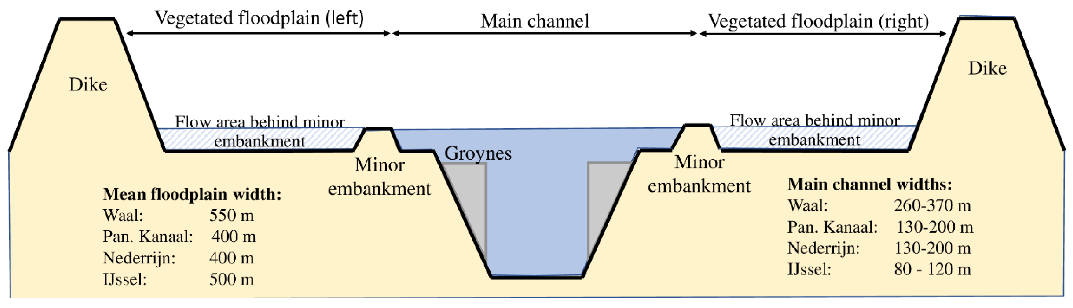
2. Domain Description

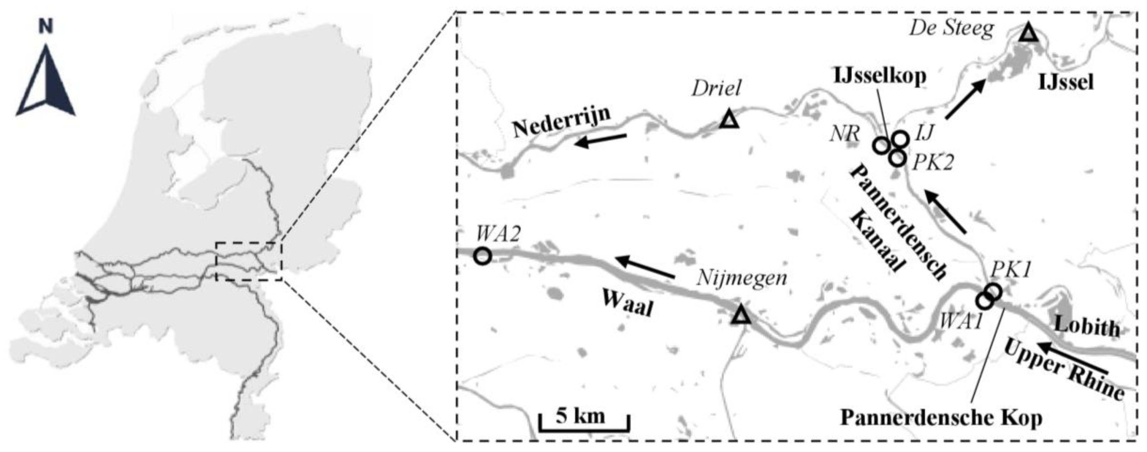
2.1. Study Area

The river Rhine bifurcates into three distributaries: the river Waal, river Nederrijn and river IJssel (Figure 1). The river Waal has the largest discharge conveyance and the largest main channel (

Table 1. Characteristics of the Dutch Rhine distributaries, based on [12,23,24].

River Branch	Bankfull Discharge (m3/s)	Width Main Channel (m)	Mean Width Floodplains (m)	Median Grain Size (D50) (mm)
Dutch Upper Rhine	5000	330–440	850	3–4
Waal	3400	260–370	550	1–2
Pannerdensch Kanaal	1600	130–200	400	3–5
Nederrijn	900	130–200	400	1–2
IJssel	700	80–120	500	2–5

). The two major bifurcation points are the Pannerdensche Kop and the IJsselkop, connected to each other by a six-kilometre long channel, the ‘Pannerdensch Kanaal’. The river Rhine enters the Netherlands at Lobith with a yearly average discharge of approximately 2200 m³/s. The bankfull discharges of the Rhine distributaries correspond to a discharge at Lobith of approximately 5000 m³/s [23]. The maximum attainable Rhine discharge is estimated to be around 18,000 m³/s [2]. The current plan form of the Rhine branches, with its two bifurcation points, has existed since the 18th century. Ever since, the discharge distribution over the distributaries has been relatively stable at about: 2/3rd towards the Waal, 2/9th towards the Nederrijn and 1/9th towards the IJssel.

2.2. Available Bedform Measurements

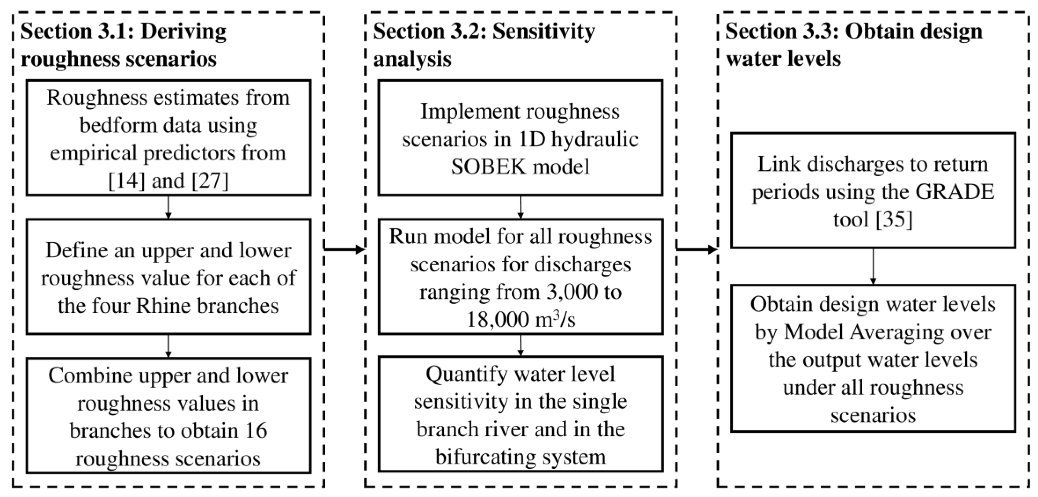
Bedform measurements for various periods of time and under different flow conditions are available (

Table 2. Characteristics of the available bedform measurements of [25,26,27]. The measurement locations are shown in Figure 1. For location WA2, measurements were taken for the northern (WA2a) and southern (WA2b) half of the main channel.

Source	# Data Points	Location	Period	Flow Regime (s)
[25]	38	WA1	1997–1998	Flood waves ’97 and ‘98
[25]	84	WA2a	1989–1998	Moderate flows & flood waves ’95, ’97 and ‘98
[25]	49	WA2b	1994–1998	Flood waves ’95, ’97 and ‘98
[25]	31	PK1	1997–1998	Flood waves ’97 and ‘98
[27]	94	WA3	2002–2003	Moderate flows
[26]	5	PK2	Jan. 2004	Moderate flows
[26]	5	IJ	Jan. 2004	Moderate flows

). The majority of these data are obtained from [25], who have used single-beam and multibeam (mostly since 1997) measurements of the river bed at the Pannerdensche Kop to derive bedform dimensions during large flood events. This data set includes records taken during the discharge wave with the highest recorded discharge in the river Rhine in 1995 as well as from flood waves in 1997 and 1998. Additionally, [26] have analysed the bedforms around the IJsselkop during a moderate flood event in 2004. Finally, [27] provides data under moderate discharges along the Waal branch. Data points from every source at least contain a bedform height and a bedform length estimate as well as the local water depth, depth-averaged flow velocity and discharge estimate.

3. Methodology

The sensitivity of water levels to variations in roughness is quantified for a single-branch river and for a bifurcating river system by modelling the water levels under various roughness scenarios (Figure 2). Therefore, in each of the four Rhine branches, a realistic upper and lower value of the roughness is estimated (Section 3.1). This results in 16 possible combinations of system roughness consisting of a high or a low roughness value for each of the branches. The sensitivity analysis is performed using the one-dimensional hydraulic model of the Rhine branches (Section 3.2). A one-dimensional model allows for fast computations, while it is sufficiently accurate for the purpose of this study. Sensitivity is defined as the difference in water levels between the scenarios in which the local branch experiences a high and a low roughness. The single-branch river and the bifurcating river are differentiated by comparing the water levels at equal local branch discharge or at equal upstream discharge, respectively. Finally, the simulated water levels are linked to return periods to obtain design water levels (Section 3.3). This shows the impact of the water-level variations in the context of flood management.

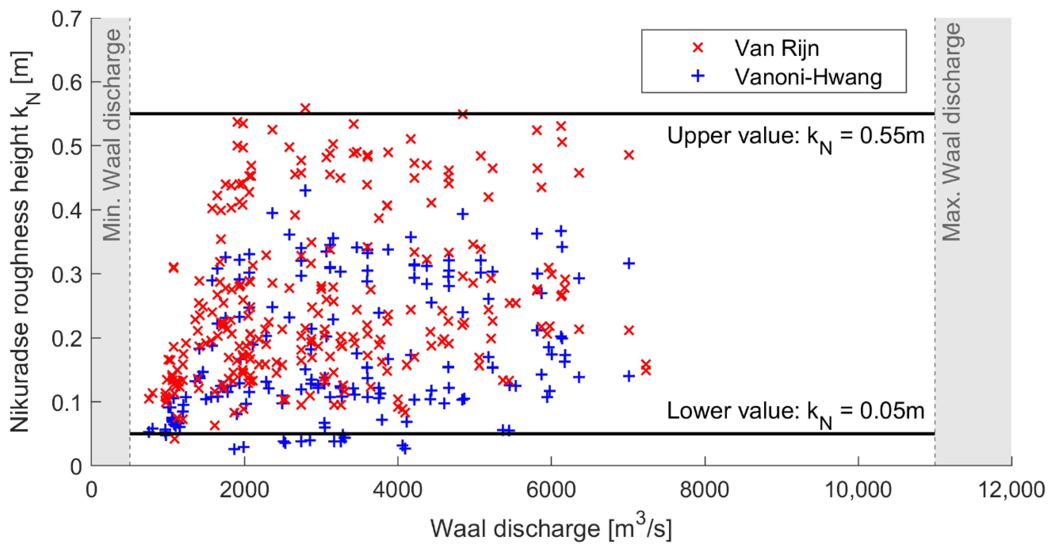
3.1. Deriving Roughness Scenarios from the Available Bedform Dimension Data

Sixteen roughness scenarios are defined that consist of combinations of an upper and a lower roughness value for each branch. These 16 scenarios represent the variability in main channel roughness in the river system. The high and low roughness value should be seen as an extreme, but realistic spread in roughness that could occur in each branch. It is not intended to give accurate predictions of roughness, given the large spread in the bedform observations, but merely to show the sensitivity of the water levels to variations in roughness. The assumptions that underlie the derivation of these roughness scenarios are discussed in Section 5.1.

The available bedform measurements are transformed into roughness values using empirical roughness predictors. The predictors of Van Rijn [15] and Vanoni-Hwang [28] are selected for this study as those showed the best performance for the Upper Rhine reach [3]. For every data sample, two roughness values are obtained, one for each of the two predictors.

The predictor of Van Rijn [15] is a function of the grain size and the bedform height and length:

$$k_N=k_{N;grains}+k_{N;forms}=3\times D_{90}+1.1\times 0.7\times \mathsf{\Delta }\times \left(1-e^{-25\mathsf{\Delta }/\Lambda }\right)$$

(1)

In addition to the bedform dimensions, the Vanoni-Hwang [28] predictor requires the magnitude of mean water levels and flow velocities:

$$c_f=\frac{1}{8}(1.8\log {\left(\frac{4uR}{7\nu }\right)}^{-2}+\frac{1}{8}{\left(3.3\log \left(\frac{\Lambda R}{{\Delta }^2}\right)-2.3\right)}^{-2}$$

(2)

The friction coefficient $c_f$ [-] can be transformed into a Nikuradse roughness height as follows:

$$k_N=\frac{12.2h}{{10}^{1/2.3\sqrt{1/\left(8c_f\right)} }}$$

(3)

In these predictors, k_N is the Nikuradse roughness height (m), D₉₀ is the 90th percentile grain diameter (m), Δ and Λ are the mean dune height and mean dune length (m), R is the hydraulic radius (m), h is the water depth (m), u is the depth-averaged velocity (m/s) and υ is the kinematic viscosity (m²/s).

The predicted roughness values that correspond to the data of the Waal branch show a large variation (Figure 3). This scatter is a result of the variation in underlying bedform dimensions and variations in the flow parameters. Generally, the Van Rijn predictor results in higher roughness values than the Vanoni-Hwang predictor. This is coherent with earlier findings of [3]. No distinct discharge-dependency of the roughness is observed in the data at Waal discharges higher than 2000 m³/s. This is not consistent with the literature e.g., [29,30] as a larger discharge is generally accompanied by larger bedform dimensions.

The same analysis is carried out for the three other Rhine river distributaries (not shown here). The predicted roughness values of the Pannerdensch Kanaal (PK) observations show a slightly lower spread in roughness values (k_N = 0.05 m up to k_N = 0.35 m). However, discharge-dependency is more pronounced with the highest roughness values occurring at the highest observed discharges. This indicates that for higher discharges, higher roughness induced by bedforms may also occur, because of the larger grain size in the PK (Table 1). For both the Nederrijn and IJssel, only 5 observations are available, all recorded in a single flood wave with moderate flows. For these observations, roughness estimates are all in the order of k_N = 0.1 m.

After visual inspection of the roughness predictions, an upper and a lower roughness value is chosen for each branch. For the Waal branch, the lower and upper value are set to k_N = 0.05 m and k_N = 0.55 m, respectively (Figure 3). In the measured discharge range, only a few predicted roughness values fall outside of these values. The chosen upper value does not account for higher roughness values outside of the measured discharge domain, because in the measured domain the roughness does not show a clear discharge-dependency.

For the other branches, the lower and upper value are set to k_N = 0.05 m and k_N = 0.55 m as well, for consistency with the Waal branch. For these branches, fewer observations are available. As the bed material and flow conditions are fairly similar in all branches (see Table 1), there is no reason to expect very different roughness values in the other branches. Additionally, the literature indicates that the bedform variability in these branches is also significant [26,27]. Therefore, the same roughness values as for the Waal and Pannerdensch Kanaal are applied.

3.2. Sensitivity Analysis Using the Hydraulic SOBEK Model of the Rhine Branches

The SOBEK modelling environment is selected to perform the sensitivity analysis. In this environment, a detailed schematization is available for the study area. This official schematization ‘Rijn-j16_5_v1′ is used by the Dutch Ministry of Infrastructure and Water Management for operational uses. SOBEK is a modelling environment [31] for 1D hydraulic computations, numerically solving the 1D Saint-Venant equations. The river is schematized by a 1D network in which the other dimensions are assigned by imposing cross-sections. Cross-sections are divided into different parts, e.g., left and right floodplains and the main channel. Furthermore, the presence of minor embankments on the floodplains is accounted for by the addition of flow area in the floodplain area (Figure 4). The governing equations are solved for the different parts separately and, after iteration, the division of discharge between the different parts of the cross-section is found. This allows for different flow velocities in the floodplains and the main channel.

The model schematization has cross-sections with a longitudinal spacing of approximately 500 m. A schematisation of a typical cross-section is shown in Figure 4. In an earlier study [32], the cross-sections were extracted from a 2D model, which is based on digital elevation maps constructed from echo-sounds in the main channel and Lidar measurements in the floodplains. After extracting the cross-sections from the 2D model, the cross-sectional dimensions were modified, such that such that modelled stage-discharge relationships match those of the 2D model [32]. Each cross-section is associated with discharge-dependent Chezy roughness values for the floodplains. The floodplains of the Rhine distributaries are vegetated, mostly with grass, but also with higher and denser vegetation. They are mainly used for agriculture and nature conservation and are regularly managed for those purposes. The roughness values are based on vegetation maps, vegetation roughness descriptions and two-dimensional model simulations [3,33]. In an earlier study, the 2D model simulations were used as reference case for the calibration of the floodplain roughness in the 1D SOBEK model [32]. Generally, Chezy values roughness are around 40 m^1/2/s at lower discharges and 50 m^1/2/s at higher discharges.

The upstream boundary of the model is located just upstream of Lobith in the Upper Rhine (Figure 1). The downstream boundary of each branch consists of a stage–discharge relation based on measurements. These boundaries are located more than 60 km downstream of the area of interest, which is sufficiently far away to not influence the water levels in the area of interest (Figure 1).

The roughness scenarios are implemented in the original schematization of the Rhine branches. In the original schematization, the main channel roughness is calibrated to attain measured water levels for a measured discharge distribution over the branches. The defined main channel roughness scenarios replace these calibrated values of main channel roughness. The roughness of the floodplains are kept at their calibrated values. Because the main channel roughness values are adapted in the scenario runs, they no longer correspond to their calibrated values. This caused shifts in the stage-discharge relationships. To attain values for water levels and bankfull discharges that are in the same order as the values from the calibrated model, a constant additional roughness wad added in all branches. This additional roughness accounts for all roughness inducing processes that are not accounted for in the model schematization, such as the flow resistance caused by groynes. A value of k_N,rest = 0.3 m for all branches gives the best match with results from the original, calibrated model schematization (i.e., “Rijn-j16_5_v1”). To find this best match, the water levels averaged over all scenarios were compared with the results from the calibrated model. This value is added to the roughness of the main channel on top of the adopted roughness scenarios. This gives a constant low roughness value of k_N = 0.35 m and a constant high roughness value of k_N = 0.85 m for all branches. In summary, the floodplain roughness values remain at their calibrated values, while the main channel roughness values under the roughness scenarios are realistic compared to the fully calibrated model by the addition of a constant roughness.

The model is run for every of the 16 roughness scenarios. To assess the sensitivity of the water levels to discharge, the model is run for every scenario with constant discharges ranging from 3000 m³/s (above yearly-averaged discharge) up to 18,000 m³/s (maximum discharge at Lobith; see [2]) with steps of 500 m³/s. This gives a total amount of model runs of 496 (31 discharges and 16 roughness scenarios). The sensitivity to roughness at a certain discharge is defined as the mean difference in water levels between the scenarios in which the local branch experiences a high roughness (H) and a low roughness (L), respectively:

$$Sensitivity \left(Q\right)=\overline{H_{Waal}\left(Q\right)-L_{Waal}\left(Q\right)}$$

(4)

Here, the differentiation is made between a single-branch river and a bifurcating river system. In the single-branch river system, the sensitivity to roughness is assessed at equal discharge inside the branch. In contrast, in the bifurcating river system, the sensitivity is assessed at equal upstream Lobith discharge, thereby allowing for variations in the discharge distribution under the various roughness scenarios.

3.3. Obtaining Design Water Levels (DWLs) Using Model Averaging

The return periods of modelled water levels are determined for the three locations of interest (Figure 1) for the single-branch river and for the bifurcating river system. Model averaging (MA) is applied to combine the model results under the various scenarios into a single new model result. MA has been widely used in the field of hydrology [34] and recently MA has been used in river flood modelling as well [35]. Furthermore, it is common practice under the Dutch flood risk framework to apply MA to account for uncertainties, while still having a single model prediction [36]. MA is used to determine the average probability over all 16 scenarios of water level h occurring p(h):

$$p\left(h\right)={\displaystyle \sum }_{m_i}p(m_i)\times p(h|m_i)$$

(5)

Here, $p\left(m_i\right)$ is the probability of occurrence of a roughness scenario and $p\left(h\right|m_i)$ is the probability of water level h occurring under roughness scenario $m_i$. It is assumed that every roughness scenario is equally likely to occur, so:

$$\begin{gathered} \mathrm{For} \mathrm{the} \sin \mathrm{gle}-\mathrm{branch} \mathrm{river}:p\left(m_i\right)=0.5; \mathrm{for} i=1:2 \\ \mathrm{For} \mathrm{the} \mathrm{bifurcating} \mathrm{river}:p\left(m_i\right)=0.0625; \mathrm{for} i=1:16 \end{gathered}$$

(6)

The return periods from the modelling tool ‘Generator of Rainfall and Discharge Extremes’ (GRADE) are used for this analysis [37]. In the Netherlands, this tool is used in operational practices by the Dutch Ministry of Infrastructure and Water Management. Using these data, the return periods of input upstream discharges ranging from 3000 to 18,000 m³/s are obtained. For the single-branch river system, branch discharges are coupled to the upstream discharge and their return periods by taking the mean discharge distribution over all 16 scenarios.

4. Results

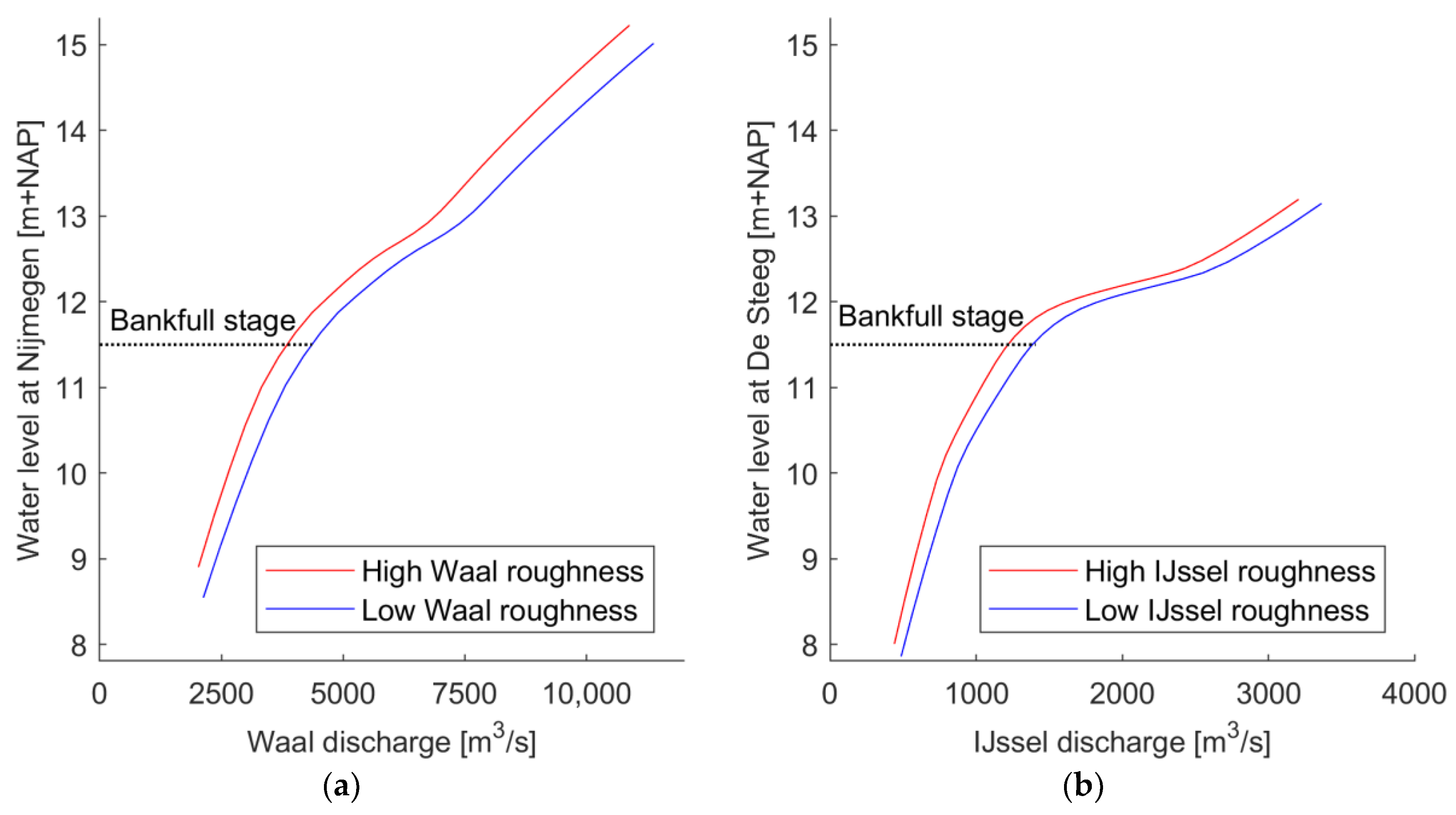
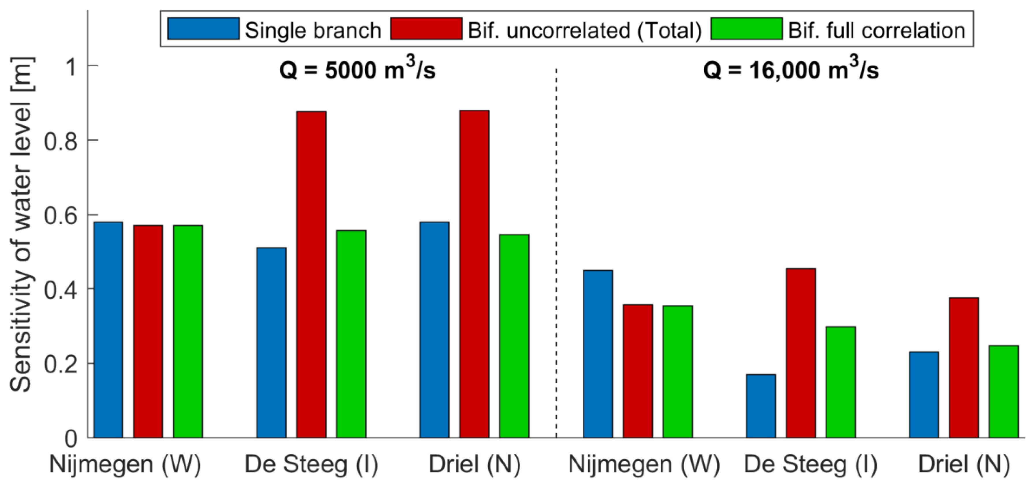
4.1. Sensitivity to Roughness in a Single-Branch River

The results show that the imposed roughness scenarios induce large changes to the local stage–discharge relationships at the two locations in the Waal and IJssel branches (Figure 5), representing the sensitivity of single-branch rivers for roughness variations. Averaged over all discharges, the difference between the water levels under the high roughness estimates and the water levels under the low roughness estimate shows water levels of 0.4 m higher at Nijmegen (Waal) and 0.3 m higher at De Steeg (IJssel). Similar sensitivities to the roughness are found for the location of Driel (Nederrijn). These values are in the same order of magnitude as values of water-level uncertainties caused by roughness uncertainty that were previously found in literature, e.g., a 95% confidence interval of 0.53 m at the design discharge in the Waal river [3] and 95% confidence intervals of 0.3–1.0 m in the Po and Garonne river [10].

The modelled shapes of the stage-discharge relationships are typical for a lowland river with floodplains (see schematized cross-section in Figure 4). Under bankfull stages, marked in Figure 5, the stage–discharge relationship is steep. Once the water level exceeds the height of the minor embankments, the floodplains start accommodating discharge, causing flattening of the stage-discharge relationship. The flattening of the stage-discharge relationship is more pronounced for the IJssel than for the Waal branch, as the floodplains of the IJssel branches are relatively wider than those of the Waal branch (Table 1).

For single-branch rivers, the sensitivity of water levels to the roughness varies as a function of discharge. The highest sensitivity is around the bankfull stage with a maximum of 0.61 m at Nijmegen and 0.58 m at De Steeg (Figure 5). The lowest sensitivity is found at conditions where the floodplains start accommodating a larger portion of the discharge (6500 m³/s in the Waal and 2500 m³/s in the IJssel), with a minimum of 0.22 m at Nijmegen and 0.10 m at De Steeg. Above the bankfull stage, the sensitivity is lower. For very high discharges (>7500 m³/s in the Waal and >2700 m³/s in the IJssel) the sensitivity to roughness is relatively constant with a value 0.45 m at Nijmegen and 0.20 m at De Steeg.

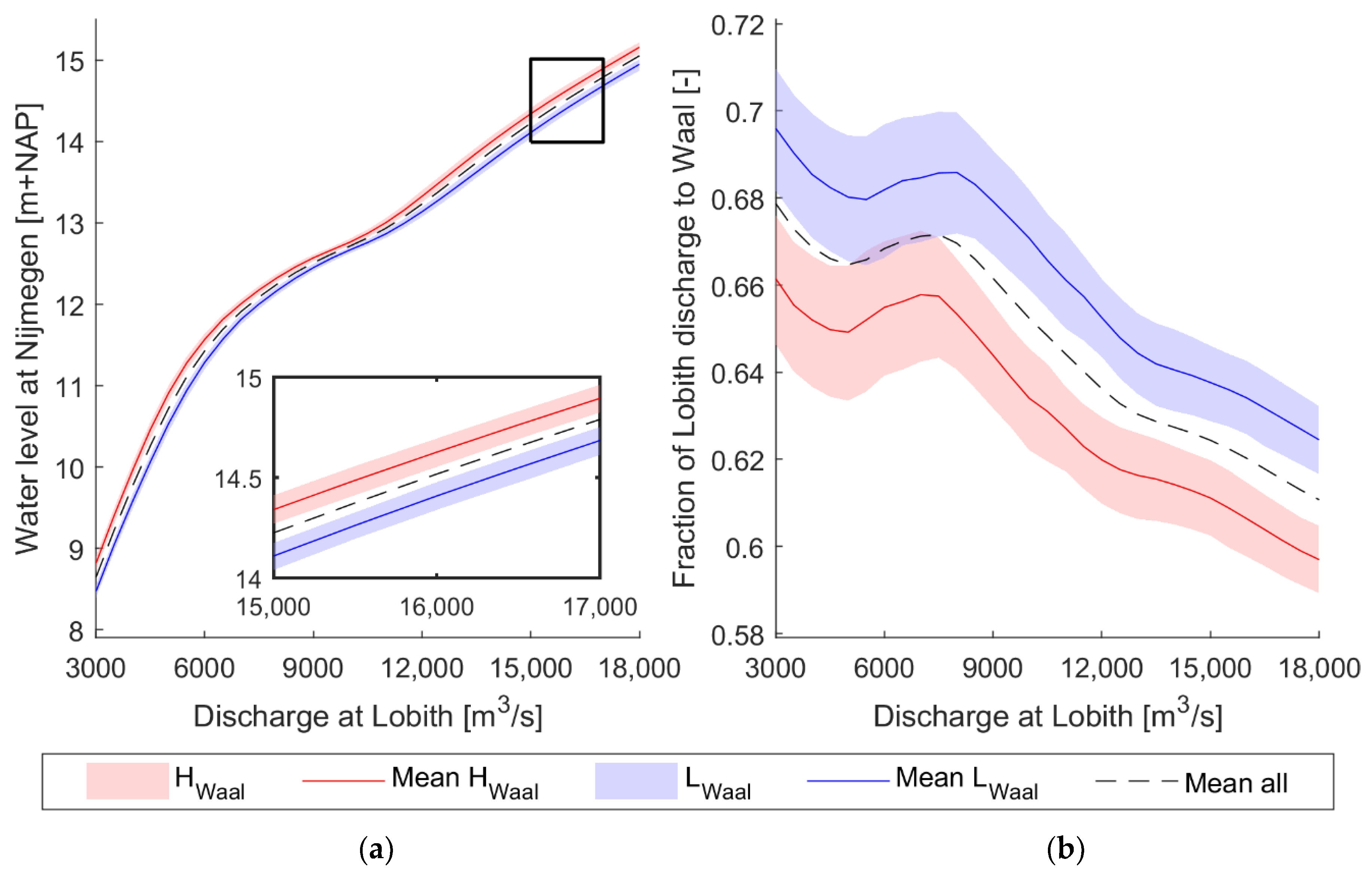
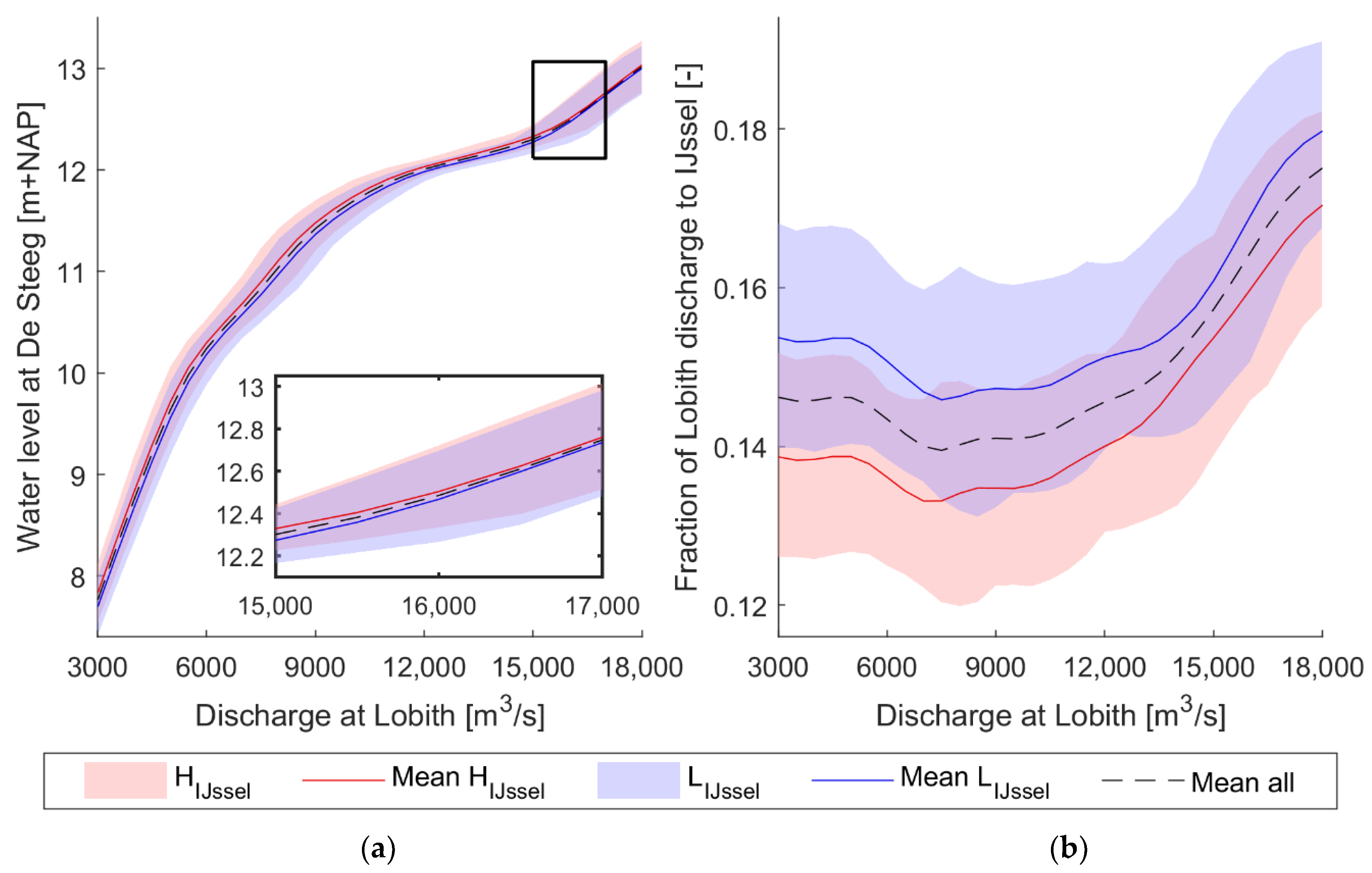
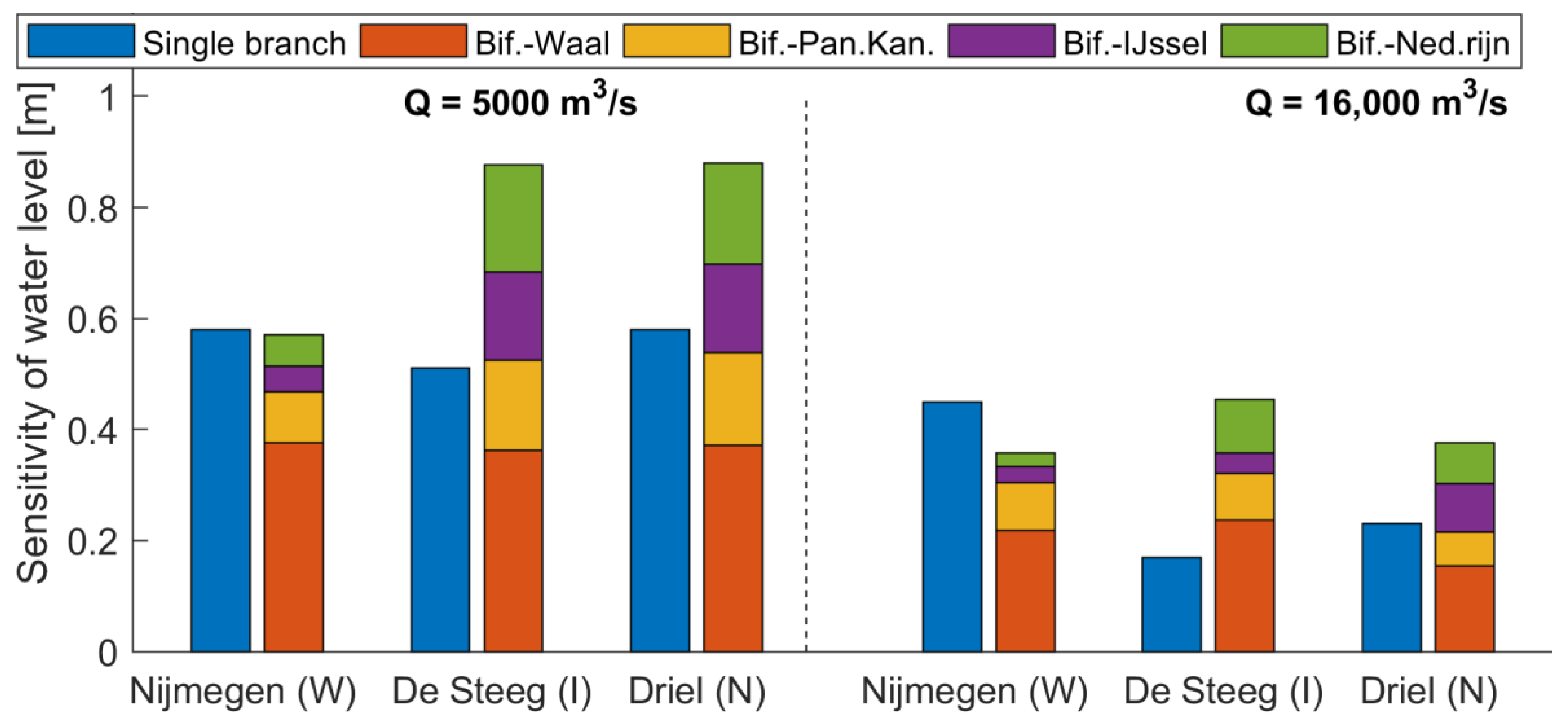
4.2. Sensitivity to Roughness in a Bifurcating River System

In a bifurcating river system, the model results show that changes in the discharge distribution at the Pannerdensche Kop, indirectly induced by the roughness variations in all branches, have a strong effect on the water levels at Nijmegen (Figure 6). Averaged over all discharges, the sensitivity of the water levels at Nijmegen to Waal roughness is 0.2 m in this bifurcating river system, while it was 0.4 m in the single-branch river. Minimum and maximum sensitivities are 0.09 m and 0.40 m, which occur at discharges that correspond to the same branch discharges as in the single-branch river, but in this single-branch river the minimum and maximum values were 0.22 m and 0.61 m. At higher discharges, the sensitivity is relatively constant at 0.21 m, while this was 0.45 m in the single-branch river. So, at all discharges, the sensitivity of the water levels to Waal roughness has been reduced, in comparison to the single-branch river, with approximately 0.2 m.

The reduced sensitivity in the bifurcating system compared to the single-branch river is associated with approximately 3% differences in Lobith discharge diverted towards the Waal (right panel of Figure 6). The effect of roughness variations on the ratio of the discharge distribution between the branches is nearly equal for all Lobith discharges. This implicates that absolute discharge variations linearly increase with upstream discharge, e.g., on average a difference of 155 m³/s and 440 m³/s at upstream discharges of 5000 m³/s and 16,000 m³/s, respectively.

At De Steeg in the IJssel branch, the difference in response of water levels to roughness variations between the bifurcating river and the single-branch river are even more pronounced. In the bifurcating system, water levels at De Steeg are insensitive to the local (IJssel) roughness (Figure 7). The sensitivity to IJssel roughness varies between 0.03 m (at Q_Lob = 18,000 m³/s) and 0.16 m (at Q_Lob = 5000 m³/s), while the sensitivity varied between 0.10 m and 0.58 m in the single-branch river. Still, looking at the overall water-level variations, these exceed the variations in the single-branch river. The difference between the best and worst case roughness scenarios ranges reaches a maximum value of 0.88 m (at Q_Lob = 4500 m³/s), while it also exceeds 0.5 m at extremely high discharges (>16,000 m³/s). These large water-level variations are induced by the deviations in the discharge distribution (right panel of Figure 7).

The response of water levels to changes in roughness in a bifurcating river system is thus different from a single-branch river (Figure 8). As seen in Figure 5, Figure 6 and Figure 7, sensitivity to roughness is higher around the bankfull discharge (5000 m³/s) than at larger discharges, at which floodplains accommodate a portion of the discharge. In the bifurcating river, water levels are a function of the roughness of all branches. However, the contribution of the branches to the total water-level variation is not equal, illustrated by the unequal height of the bars. The water levels at every location are most sensitive to the roughness in the Waal branch, illustrated by the red bars being higher than the other bars of the bifurcating system. Oppositely, the roughness of the smaller branches has little influence on the water levels in the larger Waal branch, as expected. Notably, the maximum sensitivity in the bifurcating river system (total height of the bars) even exceeds the single-branch values (blue bars) for the smaller IJssel and Nederrijn branches. However, this is only reached under specific roughness conditions, e.g., a very high discharge in the IJssel occurs if the Waal has a high roughness, while the Pannerdensch Kanaal has a low roughness. A change in roughness in the Waal branch can almost offset the water-level variations caused by all other branches (equally high bars).

Concluding, the model results showed that the sensitivity of water levels to roughness is very different in a single-branch river than in a bifurcating river system. The sensitivity to local roughness is smaller in a bifurcating river system due to changes in the discharge distribution over the branches. However, the smaller branches of the system experience large water-level variations that are related to the variations in discharge distribution. These discharge effects can exceed the local effects of roughness. These differences in sensitivities between a single-branch river and a bifurcating river system are important for flood-risk assessments. Next, the impact of these differences on design water levels is assessed.

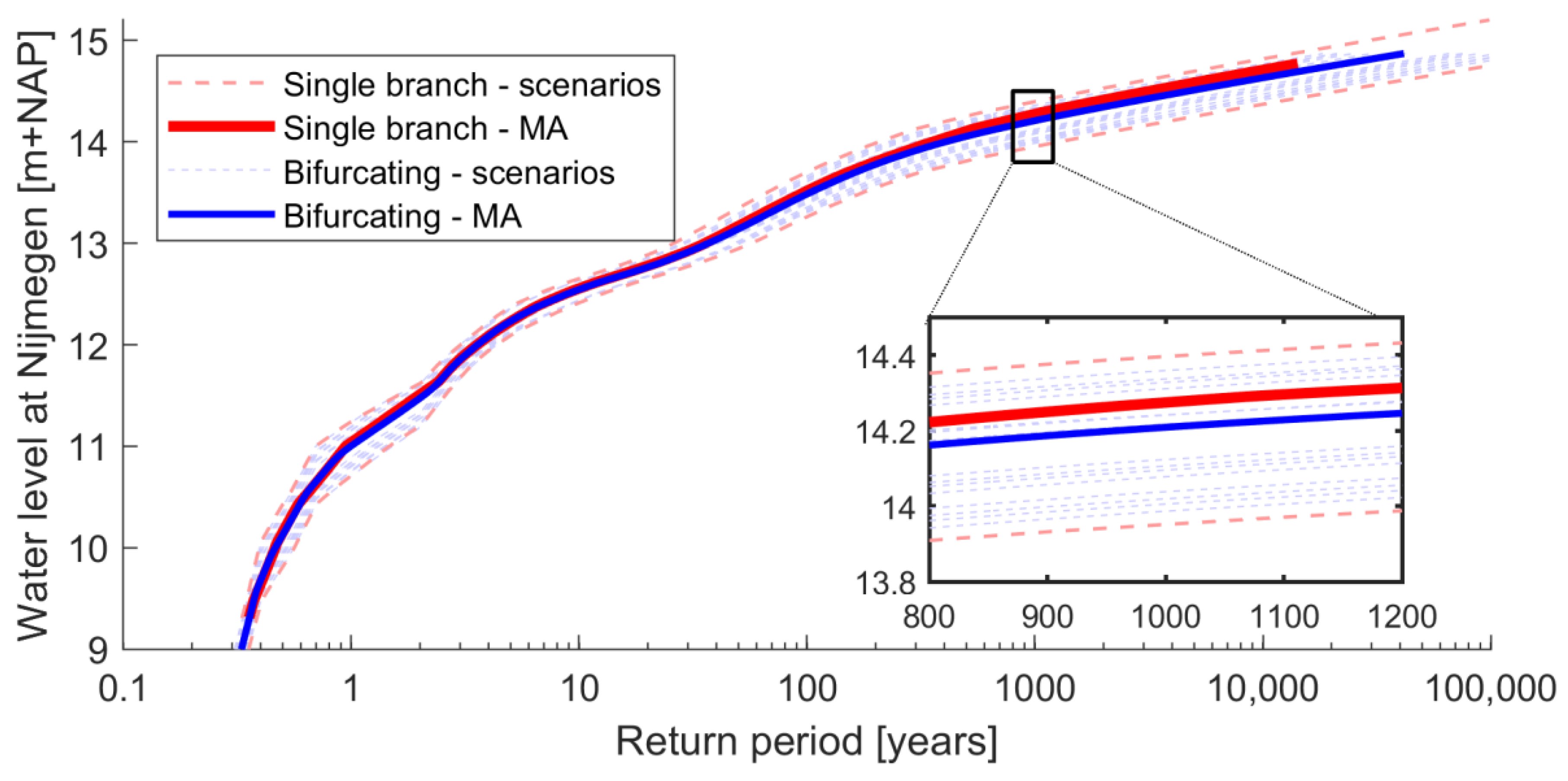
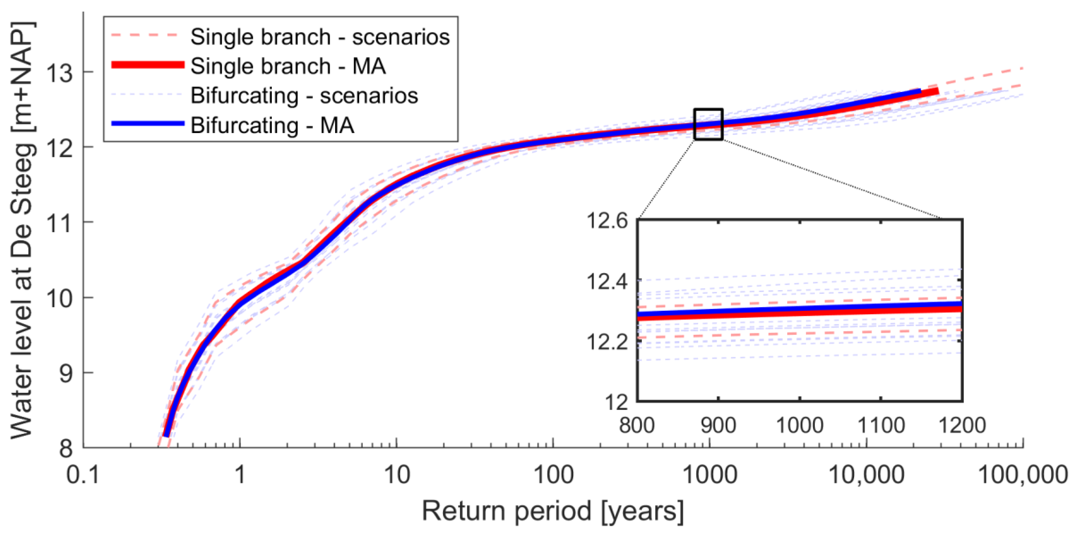
4.3. Impact on Design Water Levels

Using model averaging, DWLs are determined at the three locations (Figure 1) for the single-branch river case and for the bifurcating river case. Due to different degrees of water-level uncertainty, the DWLs are different in a bifurcating river system than in a single-branch river (

Table 3. Change in design water levels (DWL) at different return periods (T) at the three locations if comparing the bifurcating river system (bif.) to the single-branch river cases.

ΔDWL (Bif.–Single)	Nijmegen (Waal)	De Steeg (IJssel)	Driel (Nederrijn)
T = 100 years	−3 cm	−1 cm	+1 cm
T = 1000 years	−6 cm	+1 cm	−2 cm
T = 10,000 years	−8 cm	+5 cm	−1 cm

).

In the Waal branch, design water levels are lower in a bifurcating river system than in the single-branch Waal river (Figure 9). Water-level uncertainties in this branch, are smaller in the bifurcating system than in the single-branch river (Figure 8). This can also be seen in Figure 9 as all blue dashed lines lie between the dashed red lines.

Contrarily, for the IJssel branch, the DWLs are generally higher in the bifurcating river system than in the single-branch IJssel river (Figure 10). This is caused by the higher water-level uncertainties in the bifurcating river system than in the single-branch river (Figure 8). The small IJssel branch is more sensitive to the discharge variations than the larger Waal branch. In Figure 10, many of the roughness scenarios (blue dashed lines) now fall outside of the single-branch scenarios (red dashed lines).

5. Discussion

5.1. Roughness Scenarios

In this study, roughness scenarios are defined on the basis of available data on observed bedform characteristics in the four Dutch Rhine branches. These scenarios represent a realistic estimate of variations in roughness, as roughness predictions from observations and values derived in the literature [26,29] fall within the defined roughness values. Due to limited data availability in the Pannerdensch Kanaal, IJssel and Nederrijn branches, it is assumed that the bedform dynamics in the Waal river are also a good representation of the bedform dynamics in the other branches. Additional measurements of bedform dimensions in mainly the Nederrijn and IJssel branch can show the validity of this assumption and may allow for an improvement of the roughness scenarios. These additional measurements could also show the presence of discharge-dependency, which is now not observed for the Waal branch data (Figure 3). Generally, bedforms grow with increasing discharge [16,30]. However, the relationship of form roughness with discharge is even more complex. Amongst other factors, the shape of the bedform and its lee-side angle [38] as well as the water depth [26] play an important role. While in the upper reach of the Dutch Rhine discharge-dependency is clearly present [3,29], this was not as pronounced not found for downstream locations in the Waal branch [26,29].

Consequently, a higher than assumed spread of main channel roughness may occur at high discharges. Firstly, if the main channel roughness is more discharge dependent, higher roughness values at extremely high, unobserved discharges may be expected. However, secondly, flattening of bedforms in a condition of Upper Stage Plane Bed could also occur locally [19,39], leading to a significant decrease in roughness [18]. An increased spread in roughness at higher discharges is, therefore, possible. If the spread in roughness is larger than assumed, the bandwidth of modelled water levels will become somewhat larger. However, the difference in water-level response to roughness variations between a single-branch river case and a bifurcating river can still be expected. Likely, this difference grows with a larger spread in roughness, which would also lead to larger differences in design water levels.

Another assumption in the roughness scenarios was that the main channel roughness between the branches could change independently of the other branches. However, correlation of the roughness between the branches may be expected. The primary source of possible correlation between the roughness of the branches is the history of the upstream discharge by which the bedforms have developed [25,38]. Other factors that can cause correlation between the roughness of the branches can be grain characteristics [25,26], similar cross-sectional shape [25] and the shape of the discharge wave [40]. However, differences in these factors are present in the Rhine system. For example, the Waal branch has much finer sediment than the IJssel branch and also in the Waal branch a smaller portion of the discharge is accommodated by the floodplains than in the IJssel branch. Strong correlation is, thus, not apparent.

To test the effect of correlation of roughness between the branches, results are shown for the case if full correlation of the roughness is assumed (Figure 11). This leaves two roughness scenarios: either a high roughness in every branch or a low roughness in every branch. Sensitivities of water levels to roughness would generally decrease compared to the uncorrelated case. In the bifurcating river system, correlation between the roughness of the branches means that relative roughness differences between the branches diminish. Therefore, the discharge distribution will show less variation. Due to less variation in the discharge distribution, sensitivity is much closer to the single-branch river (Figure 11). Furthermore, correlation causes the maximum water-level variation to decrease in the smaller branches of the system, which is dominated by the variations in the discharge distribution.

5.2. Uncertainty Analyses in Bifurcating River Systems

In this study, the sensitivities of water levels to roughness have been quantified using a one-dimensional SOBEK model of the Rhine branches. The 1D model results are expected to be reasonably accurate in support of the aim of this study. A two-dimensional model is preferred over a one-dimensional model if more accurate predictions of absolute water levels are required [20]. However, in this study, the focus is on differences in water levels between the scenarios. The 1D approach is expected to be able to predict these differences accurately, as the various roughness scenarios are treated similarly in the model schematization. A comparison with an earlier study of water-level sensitivity in the Waal branch [3] showed similar values of water-level sensitivity as were found in this study.

This paper has considered variability in discharge and uncertainty in main channel roughness, being the most important sources of uncertainty. Besides these sources, several other sources of uncertainty, such as floodplain roughness [33] and geometry [12], result in uncertain water-level estimates. If taking these sources of uncertainty into account, slightly larger water-level variability can be expected. Specifically at extreme discharges, uncertainty related to floodplain roughness and geometry will influence the water-level estimates. It can be expected that these sources of uncertainty show less correlation between the branches, as within a branch little correlation is observed e.g., [33] thereby inducing larger changes to the discharge distribution. Water levels modelled in a single-branch river will, therefore, increasingly be different from the water levels modelled in a bifurcating river system. This will especially be true for sources of uncertainty that may occur very locally and in the vicinity of the bifurcating point, e.g., breaching of a flood defense [2], Upper Stage Plane Bed [19] or erosion of the river bed [41]. Accounting for the feedback mechanism by modelling the full bifurcating river system is thus essential in uncertainty analyses of water levels for flood risk management.

6. Conclusions

In this paper the sensitivity of water levels to main channel roughness is quantified for the bifurcating Dutch river Rhine system. In earlier studies, the effect of roughness uncertainty was evaluated for single-branch rivers. This study shows that the feedback mechanism between downstream water levels and discharge distribution at a river bifurcation strongly affects the sensitivity of water levels to roughness variations.

The results show that in a bifurcating river system water levels are less sensitive to changes of the local roughness than in a single-branch river. Changes in the discharge distribution counteract the effects of roughness on water levels. Comparing the bifurcating river with the single-branch rivers, sensitivity to local roughness at a very high upstream discharge of 16,000 m³/s reduced from 0.45 m to 0.22 m, from 0.17 m to 0.04 m and from 0.23 m to 0.07 m, in the Waal, IJssel and Nederrijn branches, respectively. In addition to sensitivity to local roughness, water levels in the bifurcating river system are also sensitive to the roughness of the other branches. Variations in roughness in the largest Waal branch lead to large variations in water levels throughout the entire system. In contrast, variations in roughness in the smallest branch lead to little change in water levels locally, and elsewhere in the system. In the smaller branches, the discharge variations that are governed by the larger branches, can exceed the sensitivity to roughness, thereby increasing the total variability of water levels in a bifurcating river system compared to a single-branch river. At an upstream discharge of 16,000 m³/s, the total variability of water levels in the IJssel and Nederrijn branches is 0.45 m and 0.38 m respectively, clearly exceeding the single-branch values of 0.17 m and 0.23 m. These principles are generally valid for lowland bifurcating river systems. Therefore, it implies that in these systems the water levels are dominated by water-level uncertainties in the largest downstream branch, if those uncertainties occur in the vicinity of the bifurcation point.

Design water levels are different in a bifurcating river system than in single-branch rivers. In the largest branch, design water levels are lower due to the lower water-level uncertainties, while in the smallest branch design, water levels increase. Therefore, it is essential that, in river management, the river system should be modelled as one interconnected system in the analysis of the water levels along the branches. This is important for the maintenance of rivers, the assessment of flood risks as well as for the future planning of river engineering works.

References

1. Dilley, M.; Chen, R.S.; Deichmann, U.; Lerner-Lam, A.L.; Arnold, M.; Agwe, J.; Buys, P.; Kjevstad, O.; Lyon, B.; Yetman, G. Natural Disaster Hotspots: A Global Risk Analysis; The World Bank: Washington, DC, USA, 2005. [Google Scholar]
2. Bomers, A.; Schielen, R.M.J.; Hulscher, S.J.M.H. Consequences of dike breaches and dike overflow in a bifurcating river system. Nat. Hazards 2019, 97, 303–304. [Google Scholar] [CrossRef] [Green Version]
3. Warmink, J.J.; Booij, M.J.; Van der Klis, H.; Hulscher, S.J.M.H. Quantification of uncertainty in design water levels due to uncertain bed form roughness in the Dutch river Waal. Hydrol. Process. 2013, 27, 1646–1663. [Google Scholar] [CrossRef]
4. Apel, H.; Merz, B.; Thieken, A.H. Quantification of uncertainties in flood risk assessments. Int. J. River Basin. Manag. 2008, 6, 149–162. [Google Scholar] [CrossRef] [Green Version]
5. Berends, K.B.; Straatsma, M.A.; Warmink, J.J.; Hulscher, S.J.M.H. Uncertainty quantification of flood mitigation predictions and implications for decision making. Nat. Hazard Earth Sys. 2019, 19, 1737–1753. [Google Scholar] [CrossRef] [Green Version]
6. Pappenberger, F.; Beven, K.J. Ignorance is bliss: Or seven reasons not to use uncertainty analysis. Water Resour. Res. 2006, 42, W05302. [Google Scholar] [CrossRef]
7. Pappenberger, F.; Beven, K.J.; Ratto, M.; Matgen, P. Multi-method global sensitivity analysis of flood inundation models. Adv. Water Resour. 2008, 31, 1–14. [Google Scholar] [CrossRef]
8. Merz, B.; Thieken, A.H. Flood risk curves and uncertainty bounds. Nat. Hazards 2009, 51, 437–458. [Google Scholar] [CrossRef]
9. Warmink, J.J.; Van der Klis, H.; Booij, M.J.; Hulscher, S.J.M.H. Identification and quantification of uncertainties in a hydrodynamic river model using expert opinions. Water Resour. Manag. 2011, 25, 601–622. [Google Scholar] [CrossRef] [Green Version]
10. Bozzi, S.; Passoni, G.; Bernardara, P.; Goutal, N.; Arnaud, A. Roughness and discharge uncertainty in 1D water level calculations. Environ. Model Assess. 2015, 20, 343–353. [Google Scholar] [CrossRef]
11. Bomers, A.; Schielen, R.M.J.; Hulscher, S.J.M.H. Application of a lower-fidelity surrogate hydraulic model for historic flood reconstruction. Environ. Model Softw. 2019, 117, 223–236. [Google Scholar] [CrossRef] [Green Version]
12. Van Vuren, B.G.; De Vriend, H.J.; Ouwerkerk, S.; Kok, M. Stochastic modelling of the impact of flood protection measures along the river Waal in the Netherlands. Nat. Hazards 2005, 36, 81–102. [Google Scholar] [CrossRef]
13. Klijn, F.; Asselman, N.E.M.; Mosselman, E. Robust river systems: On assessing the sensitivity of embanked rivers to discharge uncertainties, exemplified for the Netherlands’ main rivers. J. Flood Risk Manag. 2018, 12, e12511. [Google Scholar] [CrossRef]
14. Ardıçlıoğlu, M.; Alban Kuriqi, A. Calibration of channel roughness in intermittent rivers using HEC-RAS model: Case of Sarimsakli creek, Turkey. SN Appl. Sci. 2019, 1, 1080. [Google Scholar] [CrossRef] [Green Version]
15. Van Rijn, L.C. Principles of Sediment Transport in Rivers Estuaries and Coastal Areas; Aqua Publications: Blokzijl, The Netherlands, 1993. [Google Scholar]
16. Julien, P.Y.; Klaassen, G.J. Sand-dune geometry of large rivers during floods. J. Hydraul. Eng. 1995, 121, 657–663. [Google Scholar] [CrossRef]
17. Best, J. The fluid dynamics of river dunes: A review and some future research directions. J. Geophys. Res. 2005, 110, F04S02. [Google Scholar] [CrossRef]
18. Nelson, J.M.; Logan, B.L.; Kinzel, P.J.; Shimizu, Y.; Giri, S.; Shreve, R.L.; McLean, S.R. Bedform response to flow variability. Earth Surf. Process. Landf. 2011, 36, 1938–1947. [Google Scholar] [CrossRef]
19. Hulscher, S.J.M.H.; Daggenvoorde, R.J.; Warmink, J.J.; Vermeer, K.; Van Duin, O. River dune dynamics in regulated rivers. In Proceedings of the 4th International Symposium on Shallow Flows, Eindhoven, The Netherlands, 26–28 June 2017. [Google Scholar]
20. Berends, K.B.; Warmink, J.J.; Hulscher, S.J.M.H. Efficient uncertainty quantification for impact analysis of human interventions in rivers. Environ. Model Softw. 2018, 107, 50–58. [Google Scholar] [CrossRef] [Green Version]
21. Jansen, P.P.; Van Bendegom, L.; Van den Berg, J.; De Vries, M.; Zanen, A. Principles of River Engineering: The Non-Tidal Alluvial River; Delftse Uitgevers Maatschappij: Delft, The Netherlands, 1979. [Google Scholar]
22. Ciullo, A.; De Bruijn, K.M.; Kwakkel, J.H.; Klijn, F. Systematic flood risk management: The challenge of accounting for hydraulic interactions. Water 2019, 11, 2530. [Google Scholar] [CrossRef] [Green Version]
23. Reeze, B.; Van Winden, A.; Postma, J.; Pot, R.; Hop, J.; Liefveld, W. Watersysteemrapportage Rijntakken 1990–2015; Ontwikkelingen Waterkwaliteit en Ecologie; Bart Reeze Water & Ecologie: Harderwijk, The Netherlands, 2017. [Google Scholar]
24. Brilhuis, R. Enkele Hydraulische en Morfologische Parameters van de Nederlandse Rijntakken; Rijkswaterstaat: Arnhem, The Netherlands, 1988. [Google Scholar]
25. Wilbers, A.W.E.; Ten Brinke, W.B.M. The response of sub-aqueous dunes to floods in sand and gravel bed reaches of the Dutch Rhine. Sedimentology 2003, 50, 1013–1034. [Google Scholar] [CrossRef]
26. Frings, R.M.; Kleinhans, M.G. Complex variations in sediment transport at three large river bifurcations during discharge waves in the river Rhine. Sedimentology 2018, 55, 1145–1171. [Google Scholar] [CrossRef]
27. Sieben, J. Taal van de Rivierbodem; Rijkswaterstaat: Lelystad, The Netherlands, 2008. [Google Scholar]
28. Vanoni, V.A.; Hwang, L.S. Relation between bedforms and friction in streams. J. Hydraul. Div. 1967, 93, 121–144. [Google Scholar]
29. Julien, P.Y.; Klaassen, G.J.; Ten Brinke, W.B.M.; Wilbers, A.W.E. Case study: Bed resistance of Rhine river during 1998 flood. J. Hydraul. Eng. 2002, 128, 1042–1050. [Google Scholar] [CrossRef] [Green Version]
30. Paarlberg, A.J.; Dohmen-Jansen, C.M.; Hulscher, S.J.M.H.; Termes, A.P.P.; Schielen, R.M.J. Modelling the effect of time-dependent river dune evolution on bed roughness and stage. Earth Surf. Process. Landf. 2010, 35, 1854–1866. [Google Scholar] [CrossRef]
31. Deltares. SOBEK3, D-Flow 1D User Manual Version 3.4.0; Deltares: Delft, The Netherlands, 2020. [Google Scholar]
32. Becker, A.; Scholten, M.; Kerkhoven, D.; Spruyt, A. Das behördliche Modellinstrumentarium der Niederlande. In Dresdner Wasserbaukolloquium 2014 Simulationsverfahren und Modelle für Wasserbau und Wasserwirtschaft; Stamm, J., Ed.; Dresden University of Technology: Dresden, Germany, 2014; pp. 539–548. [Google Scholar]
33. Straatsma, M.W.; Huthoff, F. Uncertainty in 2D hydrodynamic models from errors in roughness parameterization based on aerial images. J. Phys. Chem. Earth 2011, 36, 324–334. [Google Scholar] [CrossRef]
34. Parrish, M.A.; Moradkhani, H.; DeChant, C.M. Toward reduction of model uncertainty: Integration of Bayesian model averaging and data assimilation. Water Resour. Res. 2012, 48, W03519. [Google Scholar] [CrossRef]
35. Liu, Z.; Merwade, V. Accounting for model structure, parameter and input forcing uncertainty in flood inundation modeling using Bayesian model averaging. J. Hydr. 2018, 565, 138–149. [Google Scholar] [CrossRef]
36. Diermanse, F.L.M. Overzichtsrapport Onzekerheden: Overzicht van Belasting- en Sterkte-Onzekerheden in Het Wettelijk Beoordelingsinstrumentarium; Deltares: Delft, The Netherlands, 2017. [Google Scholar]
37. Prinsen, G.; Van den Boogaard, H.; Hegnauer, M. Onzekerheidsanalyse Hydraulica in GRADE; Deltares: Delft, The Netherlands, 2015. [Google Scholar]
38. De Ruijscher, T.V.; Naqshband, S.; Hoitink, A.J.F. Effect of non-migrating bars on dune dynamics in a lowland river. Earth Surf. Proc. Landf. 2020, 45, 1361–1375. [Google Scholar] [CrossRef]
39. Naqshband, S.; Ribberink, J.S.; Hulscher, S.J.M.H. Using both free surface effect and sediment transport mode parameters in defining the morphology of river dunes and their evolution to upper stage plane beds. J. Hydraul. Eng. 2014, 140, 1–6. [Google Scholar] [CrossRef]
40. Warmink, J.J. Dune dynamics and roughness under gradually varying flood waves, comparing flume and field observations. Adv. Geosci. 2014, 39, 115–121. [Google Scholar] [CrossRef] [Green Version]
41. Kleinhans, M.G.; Jagers, H.R.A.; Mosselman, E.; Sloff, C.J. Bifuration dynamics and avulsion duration in meandering rivers by one-dimensional and three-dimensional models. Water Resour. Res. 2008, 44, W08454. [Google Scholar] [CrossRef]
Figure 1. Map of the study area in the Netherlands. The three triangles indicate the representative locations for the water levels in the three downstream branches under consideration in this study. The six circles indicate the locations at which measurements of bedform dimensions are available.
Water 12 01915 g001
Figure 2. Overview of the methodology.
Water 12 01915 g002
Figure 3. Nikuradse roughness values calculated with the Van Rijn [15] and Vanoni-Hwang [28] roughness predictors for the available data in the Waal branch. The black lines indicate the defined range of roughness with an upper value and a lower value.
Water 12 01915 g003
Figure 4. Schematisation of a typical cross-section of the Rhine branches.
Water 12 01915 g004
Figure 5. Modelled stage-discharge relations, with water levels relative to the Dutch Ordnance Datum (NAP), at Nijmegen (a) and De Steeg (b) under the imposed main channel roughness scenarios. Averaged over all discharges, a high local roughness compared to a low local roughness results in 0.4 m higher water level at Nijmegen (Waal) and 0.3 m higher water levels at De Steeg (IJssel).
Water 12 01915 g005
Figure 6. Modelled water levels at Nijmegen in the Waal branch (a) and the fraction of upstream discharge towards the Waal (b) under the 16 roughness scenarios as a function of (upstream) Lobith discharge. Scenarios with low Waal roughness (blue shaded) cause relatively low water levels and high Waal discharges, while scenarios with high Waal roughness (red shaded) cause relatively high water levels and low Waal discharges.
Water 12 01915 g006
Figure 7. Modelled water levels at De Steeg in the IJssel branch (a) and the fraction of upstream discharge diverted towards the IJssel (b) under the 16 roughness scenarios as a function of (upstream) Lobith discharge. The IJssel roughness has a small effect on both the water levels and the amount of discharge diverted towards the IJssel branch.
Water 12 01915 g007
Figure 8. The sensitivity of water levels to main channel roughness in a single-branch river and in a bifurcating river system (Bif.) at upstream discharges at Lobith (Q) of 5000 and 16,000 m3/s. The shown locations are Nijmegen (Waal), De Steeg (IJssel) and Driel (Nederrijn). For every location, the single-branch sensitivity is shown, as well as the sensitivity to the roughness of every branch in the bifurcating river system.
Water 12 01915 g008
Figure 9. Water levels at Nijmegen (Waal) vs. Return period for the full bifurcating river system and for the single-branch Waal branch. The dashed lines show the individual scenarios, while the continuous lines are the model averaged (MA) lines over the single-branch scenarios (red) and over the bifurcating river system scenarios (blue).
Water 12 01915 g009
Figure 10. Water levels at De Steeg (IJssel) vs. Return period for the full bifurcating river system and for the single-branch IJssel branch. The dashed lines show the individual scenarios, while the continuous lines are the model averaged (MA) lines over the single-branch scenarios (red) and over the bifurcating river system scenarios (blue).
Water 12 01915 g010
Figure 11. Sensitivities of water levels in a bifurcating river system if the main channel roughness were fully uncorrelated or fully correlated and in a single-branch river. The bar for the uncorrelated case is the sum of the individual components for each branch (total height in Figure 8).
Water 12 01915 g011