Abstract
The identification of aquifer parameters (i.e., specific yield and hydraulic conductivity) and forcing terms (recharge) is crucial for the process of modeling groundwater flow and contamination. Inversion techniques allow the unravelling of complex systems’ heterogeneity with more ease than manual calibration by computing parameter fields through an automated minimization between simulated and measured data (i.e., water head or measured aquifer parameters). It also allows the iterative search of multiple, equally plausible solutions, depending on system complexity (e.g., aquifer heterogeneity and variability of the forcing terms such as recharge). A Zoned Adaptive Multiscale Triangulation (ZAMT) is used for parameter estimation. ZAMT is the extension of an adaptive multiscale parameter estimation procedure already applied on different field cases. This extension consists of adding constraints varying over the domain. The ZAMT dissociates the parameter grid from the calculation mesh and allows local parameter grid refinement depending on local criteria, addressing the ill-posedness of inversion problems, decreasing computation time by reducing the amount of possible solutions and local minima, and ensuring flexibility in the parameter’s distribution. Each parameter is defined per vertex of the parameter grid; it can be set with a different range of values in order to integrate more pedo-geological information and help the optimization process by reducing the number of local minima. For the same purpose, a plausibility term based on topological characteristics of the aquifer or minimal and maximal water levels is added to the objective function. Groundwater flow is described by a classical nonlinear diffusion-type equation (unconfined aquifer), which is discretized with a two-dimensional nonconforming finite element method because water head data is unsuitable to invert three-dimensional parameter fields. Therefore, flow is considered mainly horizontal, and the parameters are obtained as average values on the saturated thickness. The study area is an alluvial (unconfined) aquifer of 6.64 km², situated in the southern, Mediterranean part of France. The simulation runs with a chronicle of 191 piezometers over 7 years (2012–2019), using a calibration period of 5 years (2012–2016). The optimization threshold is set to ensure a mean absolute error below 40 cm. The ZAMT and the additional plausibility criterion were found to produce an ensemble of realistic parameter sets with low parameter standard deviation. The model is considered robust as the water head error remains at the same level during the verification period, which includes an exceptionally dry year (2017). Overall, the calibration is best near the rivers (Dirichlet boundaries), while the terraced portion of the site challenges the limits of the 2D approach and the inversion procedure.
1. Introduction
Groundwater resources management deals with both quantity and quality issues, frequently relying on mathematical models to assess and predict water flux and contamination in aquifers. Physics-based models (i.e., solving Darcy’s law, Fick’s law, mass conservation law) require a comprehensive identification of aquifer parameters (specific storage and hydraulic conductivity) over the study domain and boundary conditions (plus initial conditions in case of transient computation). As in situ measurement are scarce and costly to extend, inverse methods are a popular, if not requisite, solution to obtain parameter fields [1,2]. However, because of the poor availability of measured data, the groundwater inverse problem is ill-posed due to the number of parameters to estimate in heterogeneous natural aquifers [3,4], meaning that the solution is neither unique nor stable [5].
By reducing the dimensional space of heterogeneity, parametrization is a way to narrow down the field of solutions [6,7]. In most parametrization methods, the parameter spatial pattern is set a priori and maintained as such during the inversion procedure, such as in the case of zonation [8], deterministic [9] and/or stochastic interpolation [10,11], or a combination of both zonation and interpolation [12]. Relevant for small-scale aquifers or when heterogeneity distribution is well known [13], this approach lacks the appropriate flexibility for larger-scale systems, problems with very little available data, or intricate heterogeneity distributions. In that respect, adaptive methods make the parameter structure scalable during the minimization in order to meet the complex heterogeneity with little prior information.
As declinations of this multiscale approach, various strategies were developed: subdivision using a variance-based statistical criterion [14], identification of zonation patterns using a Kalman filter [15], nested zonation structures [16], and, more recently, sensitivity-based methods using a level set function [17,18,19]. For this project, an Adaptive Multiscale Triangulation (AMT) is deployed, enhanced with an optional zonation of the parameter boundaries (Zoned Adaptive Multiscale Triangulation, or ZAMT). This approach combines the flexibility and efficient processing of both continuity and discontinuity [20,21,22], while more effectively constraining the parametrization in regard to prior zonal geological information which assumes one parameter value per zone.
The methodology is applied to an alluvial (unconfined) aquifer (Southern France) characterized by a complex topography of the substratum. Optimization is performed by minimizing quadratic errors between simulated and observed piezometric heads and adding supplementary constraints with respect to the substratum geometry. The mathematical aspects of the method are described in Section 2; the study site characteristics and the corresponding modeling set-up are outlined in Section 3; Section 4 is dedicated to the results of the model calibration and to the discussion.
2. Groundwater Model and Calibration Procedure
2.1. The Groundwater Saturated Flow Model
Two-dimensional groundwater flow in the saturated part of the aquifer is described by a diffusion type equation, formed by the combination of Darcy’s law and the mass conservation equation, considering a constant head-over-depth assumption (Dupuit-Forchheimer’s assumption):
where S is the storativity (confined) or the specific yield (unconfined aquifer) [-], h is the groundwater head [L], T is the transmissivity tensor [L2T−1] defined by , where e is the aquifer’s saturated thickness [L] and K is the hydraulic conductivity tensor [LT−1]. F is the sink–source term [LT−1] comprising injection and/or pumping f, the groundwater recharge R, and water exchanges with the surface water [23]. This last term depends on , the water level [L] in the river; , a leakage coefficient [T−1], and , a reference head [L] defined by:
where is the riverbed elevation [L].
is the model domain; and are partitions of the domain boundaries that correspond to Dirichlet and Neumann conditions, respectively; and n is the unit vector normal to the boundary, counted positive outward. is the prescribed head value at the Dirichlet boundaries, is the prescribed flux at the Neumann boundaries, and represents the initial conditions defined over the domain. is the simulated time.
The mathematical model is solved by a two-dimensional nonconforming finite element method [24], ensuring flux continuity and mass balance (like finite volume method) and flexibility in geometry and rigorous computation of full tensor transmissivity (like conforming finite elements) [21]. The time scheme is implicit, and the unknowns are not defined at element vertices (nodes) but are average value over element edges. The equation is linearized by computing the aquifer’s saturated thickness with heads at the current time. This allows a computational time compatible with model inversion. A minimal transmissivity is imposed to handle ‘dry’ elements, i.e., elements where the water level is very close to the substratum level. It ensures hydraulic continuity and allows these elements to be wetted when the piezometric head of the elements’ neighbors increases. After discretization, the direct problem can be described by the following equation:
where h is the water head vector at the calculation time t, and F is the sink–source term vector produced at the previous time step. A is the flow coefficient matrix, depending on the mesh geometry and the parameter vector (updated explicitly, considering the variable transmissivity in the case of an unconfined aquifer).
2.2. The Groundwater Recharge and Vadose Zone Model
Recharge from precipitation is a major contributor to the sink–source terms in temperate climate [25]. Flow in unsaturated zones can be modeled through a physics-based model [26,27,28] or some more or less complex conceptual (black–grey box) models. Richards’ equation-based models are highly non-linear, difficult to integrate in an inversion procedure, and consume large amounts of computational time in real case applications. Therefore, we adopt a more conceptual model, which mimics storage and water transport by a succession of reservoirs with the one-dimensional Nash transfer function [29]:
where P is the rainfall [LT−1], ET is the actual evapotranspiration [LT−1] occurring during a time step dτ, SW is the current soil water content [L], and SWmax is the maximum soil water storage capacity [L]. I is the water [L] engaging in infiltration at time The signal is then delayed and spread, depending on the number of reservoirs N [−], the storage coefficient of reservoirs α [T], and the parameters of gamma distribution , which results in the aquifer recharge rate R [L·T−1] at the time . The integral in Equation (3) is solved numerically using the Gauss method. If the rainfall does not exceed the actual evapotranspiration and the current soil storage capacity, infiltration is null. The eventual excess of actual evapotranspiration then draws water from the current soil water content.
At the grid element level, R is multiplied by the area and by the percent of pervious surface of the element.
2.3. Model Calibration by Solving an Inverse Problem
The groundwater flow and recharge parameters are estimated through the minimization of an objective function developed within the framework of generalized weighted least squares [1,30]:
where is the objective function, P represents the vector of the parameters to be estimated, h* is the measured piezometric head, and h is the corresponding simulated value, constituting the adjusting criterion. T is the transpose operator, and W are the weighting matrices depending on measurement errors but also prioritizing optimization effort in specific locations. Because very little information about hydraulic parameters is available and considering that such values are often scale dependent [31,32], the objective function does not include a plausibility or prior information term, like the one obtained within the maximum likelihood framework. “Soft” information about the parameters is otherwise included in the parameterization of the inversion procedure (see next section).
χ is an original regularization/plausibility term (threshold criterion), which is added in order to provide more information and limit the problem of ill-posedness, especially in the context of unconfined aquifers with intricate topography. It penalizes the objective function when the computed water head is outside the limits of the aquifer, ztop being the elevation of the ground and zbot the altitude of the substratum. It must be noticed that this plausibility term can be defined over the whole domain and extended to any minimal/maximal a priori head values (not necessarily topographical information).
Due to the great number of parameters and measurements, the minimization of the objective function is led by a quasi-Newton method [21], which is less time consuming than Jacobian approaches such as Gauss–Newton methods [33]. The gradient is calculated using the discrete adjoint state method [34], while an approximation of the objective function’s Hessian is estimated thanks to the limited memory BFGS (Broyden–Fletcher–Goldfarb–Shanno) algorithm [35]. This technique allows faster computation of problems with numerous degrees of freedom, compared to standard sensitivity approaches [36], especially as the adaptive parametrization process increases the number of parameters. The stopping criteria of the algorithm are: (i) the objective function J or its gradient g are sufficiently low; (ii) the adjustment of the parameters P or the optimization of J between two iterations are too small; or (iii) the number of iterations has reached its maximum.
2.4. Zoned Adaptive Multiscale Triangulation
The parameter spatial pattern is inferred using a Zoned Adaptive Multiscale Triangulation (ZAMT), which is based on a regular AMT [20]. The triangular parameter mesh, independent of the calculation grid, draws a continuous parameter field over the whole domain by interpolation of the parameter values defined at its vertices (see Figure 1). If during the inversion process the minimization criteria are not met at the scale of a parameter cell, the latter is refined, that is, divided in 4. Refinement is halted either when the local objective function defined within a parameter grid element drops below a user-defined threshold, the number of iterations reaches a user-defined maximum, or the last iteration fails to produce a optimization better than the previous one. A detailed description of the mathematical developments and the algorithm can be found in [21] and [22].
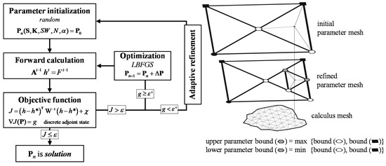
Figure 1.
The general flowchart of the inversion procedure coupled with Zoned Adaptive Multiscale Triangulation (ZAMT) parametrization.
While field measurements of the aquifer characteristics are lacking, information provided by geological and/or geophysical surveys offers an insight into large-scale zonation of the different types of porous materials. The parameter mesh is designed and adapted to integrate this a priori information: vertices’ position, density, and range of parameter values (i.e., min/max values for hydraulic conductivity and storativity/specific yield constraining the inversion) are specified according to this zonation and propagated during the refinement as shown in Figure 1. The initial parameter set and the initial values for new parameter vertices generated by subsequent refinements are picked randomly within the constraints, allowing two successive optimization runs to lead to two different solutions. Therefore, these iterative inversions can extend the sampling of the ensemble of plausible solutions. Although more exhaustive sampling methods exist, such as orthogonal or Latin hypercube sampling [37,38], they were not used here because they are very difficult to implement with scalable parametrizations.
The number of adaptive, multi-scale iterations is set to ensure a satisfactory calibration while preventing overparameterization. Meanwhile, even if technically possible, recharge parametrization is not subject to the ZAMT but to a simple static zonation because climatic data are usually prone to less spatial variability, and soil cover is usually well known.
3. Application to an Alluvial Aquifer
3.1. Description of the Study Area
The studied area is located in the south of France and consists mainly in an alluvial plain located between a stream and a major river running along its western and eastern side, with a north–south downstream orientation (see Figure 2). The northern part of the site is a succession of alluvial terraces. The highest one received colluvium (clayey sand) from the neighboring geological units, with which hydraulic communication cannot be excluded at this point. The rest of the aquifer consists of alluvial deposits (e.g., sand, gravel, pebbles, rarely consolidated).
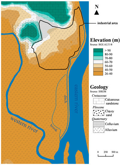
Figure 2.
The study area’s physical overview (soil topography, hydrography, geology).
The bottom of the aquifer consists of a layer of blue marls dating from the marine Pliocene era. Its mapping results from the interpolation of 793 borehole data, mainly distributed over the industrial part of the domain. It reveals that the substratum level roughly mirrors the soil surface topography (see Figure 3), apart from the middle terrace where it forms a “cuesta.” A layer of weathered marls (semi-impermeable) is observed at the bottom of the aquifer, especially in the highest terraces.
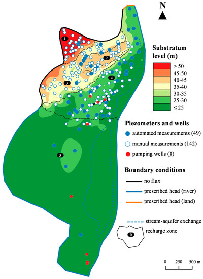
Figure 3.
The aquifer’s Characteristics used for the model (substratum level, piezometric measurements and pumping well locations, boundary conditions, and recharge zones).
Soils in the northern half of the area are heavily urbanized, that is, sealed for industrial purposes (see Figure 4), and the upper geological layers were abundantly reworked (excavation and refill) throughout the local industrial activity history. The southern half is an alluvial plain covered by loamy soils and mainly used for agriculture (vineyards).
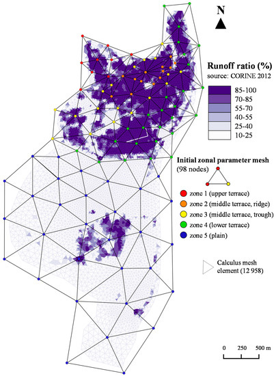
Figure 4.
The finite element mesh (with runoff ratio) and the initial ZAMT mesh.
The site is under a Mediterranean climate with mild mountain influences, characterized by a dry period of 2–3 months (June to August) and moderate yearly rainfall (around 700 mm). Daily meteorological data are acquired on site, and characteristic values for the 2012–2019 period are given in Table 1.

Table 1.
Yearly averaged meteorological data (2012–2019).
Due to the small surface area of the site (6.64 km2) and its weak topographic variations, these climatic data are considered uniform over the whole domain. The hydrographic system response to this forcing is quite heterogeneous: the eastern river, heavily impeded by dams, has a very constant water level, with an average flow rate around 1540 m3·s−1. At the western side, the stream shows much higher fluctuations (Table 2).
Table 2.
Averaged hydrographic data (source: hydrofrance).
Eight pumping wells (see Figure 3) were operating during the period of simulation, the most significant water abstractions being located in the very south of the plain, near the confluence of the bordering rivers. In the absence of precise chronicles, only average (constant) pumping rates are applied. This uncertainty will impact the parameter estimation; the wells have a local impact on groundwater levels only.
The groundwater level is monitored by a network of 191 piezometers, mainly clustered in the northern (industrial) part of the site. Forty-nine piezometers are equipped to upload hourly measurements, while 142 piezometers are subject to a biannual manual survey.
3.2. Model Conceptualization and Required Parameters
The final goal of the hydrogeological modelling is to provide an estimate of the potential impact of contamination occurring in the industrial area. This motivates an accurate modelling of the flow, taking into account non-unicity of the estimated parameters distribution. For confidentiality issues, the precise location and layout of the study area cannot be disclosed.
The comprehensive inputs required to run the inversion are reported in Table 3.
Table 3.
The model input.
The western and eastern rivers are set as Dirichlet boundary conditions with imposed, variable (over time) heads in accordance with the fluctuations drawn from the data summarized in Table 2. Exchanges between in-site streams (see Figure 3) and the aquifer are computed. The leakage coefficient is assumed to be equal to 10−8 s−1 in order to generate a low exchange rate (siltation of the riverbed).
Piezometric data in the upper and middle terrace do not demonstrate any water flux coming through the northwest boundary (fluctuations can be explained by recharge only). Therefore, if any, we assume that water fluxes can be considered as negligible, and a no-flow boundary was prescribed. Moreover, an in-site null-Neumann boundary was set to account for a man-made impermeable wall intercepting the substratum.
The northeast alluvial fringe is connected in the north to an underlying calcareous aquifer. The dynamics of the relationship between these two formations is not well established, and the water flux cannot be readily inferred. Therefore, available piezometric data at this location is used as a Dirichlet boundary condition.
Five recharge zones (see Figure 3) are defined considering the types of soils, soil cover, and the vadose zone depths, which are prone to influence the soil water storage capacity SWmax and the dynamics of infiltration.
An equivalent strategy is adopted to define the parameter mesh for the initial ZAMT, disjoining the plain and terraces parameter ranges (see Figure 4). This initial parameter mesh is based on the geology and soil surface topography, to properly discretize and set the hydrogeological parameter constraints.
The recharge and AMT zonations are also based on the analysis of precipitation and groundwater levels. Steep head gradients indicate probable low permeable zones, and small local water table fluctuations indicate probable low recharge.
The parameter values are kept within acceptable ranges (see Table 4) considering the alluvial nature of the geological domain. As the lower plain consists of the more recent deposits and is covered by agricultural soils, higher soil water storage capacities, hydraulic conductivities, and specific yields are allowed in the corresponding zone. Lower ranges of parameter values are set for the oldest geological materials (the first three zones, corresponding to the upper and middle terraces). Zone 2 parameter limits are lower than those in zone 3 due to the fact that, on the ridge, the saturated flow mainly takes place in a substratum alteration layer of low hydraulic conductivity (accounting for the presence of a piezometric dome).
Table 4.
The parameter ranges for the model inversion.
Recharge parameter ranges (see Table 4) are set in order to simulate three types of behavior: a very fast recharge (thin vadose zone) in a context of partly sealed soil (zones 1, 2, and 4), a slightly delayed recharge accounting for a thicker vadose zone (recharge zone 3), and recharge in an agricultural context with a thin vadose zone but important soil retention properties (zone 5). To alleviate the inversion effort and due to the thin unsaturated zone above the water table (and therefore expected low sensitivity to groundwater table fluctuations), the Nash gamma function parameters are fixed. A low number of Nash reservoir and a low storage coefficient (N·α < Δt) are set for zones 1, 2, 4, and 5, accounting for a reactive recharge, while higher values (Δt < N·α < 2Δt) are imposed for zone 3.
The time step for transient computation was fixed to 10 days. This time step was chosen after a detailed analysis of the water level fluctuations; neither too small (to smooth out the sharp and high variations of the piezometric heads) nor too large (to identify the impact of transient forcing such as groundwater recharge). Hydrographic and piezometric data are averaged accordingly. The chronicles of the boundary’s river head fluctuations are taken from upstream and downstream stations but leveled on the basis of onsite gauging campaigns. The water level fluctuations in the two streams within the site are inferred from the closest piezometric signals and show a pattern similar to the eastern river.
Due to extremely disparate soils conditions, the integration of the rainfall and evapotranspiration in the Nash model was conducted using two strategies. For the industrial part of the site, where the topsoil storage capacity (SWmax) is low, effective rainfall was calculated daily, then averaged over 10 days. As a result, if effective rainfall occurs on one day, the residual evapotranspiration of the time step is neglected, and only clusters of 10 days without effective rainfall can remove water from the soil (i.e., decrease water content), keeping the influence of soil storage capacity very low. On the other hand, for the agricultural part of the domain, where the soils show significant retention properties, the rainfall and the evapotranspiration are averaged separately and used as such in the Nash equations. That way, the evapotranspiration and the soil storage capacity can express to their maximum level at the decadal time step.
Concerning piezometric data, the period covered by the available chronicles was split into a calibration phase (January 2012 to October 2016) and a verification phase (November 2016 to October 2019). The calibration phase relies on 7648 head values (10-day averaged water head) mainly produced by automated measurements in piezometers. The measurements did not show any significant auto-correlation at a decadal time step. Moreover, the ponderation matrix is set to ensure a sufficient influence of the biannual surveys, otherwise dwarfed by the continuous data: each control point weight is normalized based on the number of measurements available at this location. The automatic measurements are assigned with a weight still three times higher so as not to lose the information on the short-term variations they carry. Moreover, ponderation is used to stress the importance of piezometers located in the cuesta and its surroundings (with a weight multiplied by 6), where the hydrogeological setup is the most challenging for the 2D inversion procedure and where, incidentally, the industrial stakes are the highest.
4. Results and Discussion
For comparison purposes, the inversion procedure was performed 500 times with the threshold criterion χ activated and 150 times without it. The corresponding software was developed at the Laboratory of Hydrology and Geochemistry, Strasbourg (LHyGeS). The source code is written in Fortran 90. The computations were run on a PC with Intel(R) Core(TM) i7-6700 CPU @ 3.40 GHz processor and 16 Go RAM. One model inversion lasted 3 h on average.
4.1. Topographic Constraint (Criterion χ) Contribution
By comparing two inversion populations of equal size (150), the threshold criterion χ was found successful at fulfilling its primary purpose of restraining computed water head within the aquifer’s physical boundaries (Table 5). Both number of occurrences and magnitude of violations of the substratum limit were greatly reduced. However, it significantly increased the number of parameters required for the model calibration by the ZAMT procedure (1578 compared to 871 on average).
Table 5.
The influence of the χ criterion on the substratum limits’ violations.
The criterion χ input is particularly effective in the upper terrace and cuesta areas, as well as in the terrace transitions where piezometric data are insufficient to constrain water head at levels consistent with the intricate substratum topography. By improving the simulation in areas where piezometric data is scarce but of importance for the model’s global behavior, such as the substratum crest (zone 2), the criterion produces more realistic flow directions.
The additional plausibility term also leads to a better estimation of the measured piezometric heads. For the set of 150 solutions, the smallest difference between computed and measured heads is 0.35m with the plausibility term and 0.44 without. The average difference between computed and measured heads is 0.43 m with the plausibility term and 0.55 m without.
4.2. Choice of the Adjusting Criterion Threshold and Parameter Reliability
As pointed out previously, the χ criterion allowed guiding the optimization toward a better minimum in the space of solutions. Amongst the 500 solutions, we decided to select the ones with an average quadratic error of less than 0.40, which is a compromise between accurate model calibration (i.e., low value of the objective function) and the number of solutions remaining (158 solutions for this threshold value). Defining this threshold value a priori is not an easy task since it depends on model errors (e.g., concepts and forcing terms), measurement errors (quite small compared to the previous type of errors), and scale effects due to the model discretization in space and time. Therefore, the value of 0.40 was set only after screening the solutions. For comparison purposes, the analysis was also done on a set of 438 solutions meeting the adjusting threshold of 0.5 m.
The hydraulic parameters of these solutions were analyzed by computing their average and their Relative Standard Deviation (RSD, the ratio between the standard deviation and the average, also called coefficient of variation) at each grid element. The spatial distributions of these statistical values are shown in Figure 5. The RSD is an indicator of the of the estimated parameter reliability, that is, a low value indicates that the parameter variations amongst the different solutions are small.
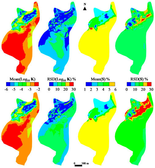
Figure 5.
Parameter values (mean and Relative Standard Deviation—RSD) for two sets of solutions (top: 40 cm threshold; bottom: 50 cm threshold).
Thanks to the ZAMT, heterogeneities in each zone remained within an acceptable order of magnitude, consistent with the alluvial context of the area. The adaptive parametrization also managed to capture the sharp transitions between the geological terraces. Despite its larger size due to the relaxing of the adjusting threshold, the set of 438 solutions showed wider parameter dispersion, especially with respect to the specific yield. This result confirms that the chosen criterion narrows down the calibration towards a set of consistent solutions. The RSD of the hydraulic conductivities (in decimal log) was almost everywhere beneath 15%, and it was particularly low on the upper and middle terraces. Spots of higher dispersion occurred for both conductivity and specific yield at the terrace transitions where interpolation captured a wider range of parameter values from two different zonations.
The soil water storage capacity distribution followed the same pattern: the lower the error threshold, the lower the dispersion (Table 6).
Table 6.
Soil water storage capacity values (mean and RSD) for each zone and for the two sets of solutions.
Moreover, it was verified that the 158 selected solutions form a sufficiently large population by comparing its statistical characteristics with those of a subset of 79 solutions. The absolute difference for each element was distributed as shown in Figure 6. Mean parameter fields showed very little discrepancy (below 0.02 decimal log unit for 90% of hydraulic conductivity values and never more than 0.001 for specific yields). The very small difference in RSD between the set and its subset demonstrates that the pool of 158 solutions can be considered as large enough (additional solutions would not significantly decrease the parameter dispersion).
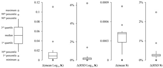
Figure 6.
A statistical comparison between the complete set (158) and a subset of solutions (79).
The analysis of parameter estimation can also be supported by the parameter distribution over a specific area. The histograms of the hydraulic parameters by zones are depicted in Figure 7. Specific yields showed overall normal pattern distribution. Concerning the hydraulic conductivities, the distributions tended to pack towards the parametrization’s highest limit in zones 1, 3, and 5. In zone 5 (agricultural plain), 0.01 m·s−1 of hydraulic conductivity was considered as a realistic maximum in a natural alluvial context. The distribution produced by the inversion could be compensating boundary condition uncertainties (prescribed head and exchanges with rivers). For zone 2 (the middle terrace ridge), the values stick to the lower limit, which is consistent with the saturated zone being mainly in a clayey layer (resulting from the substratum alteration).
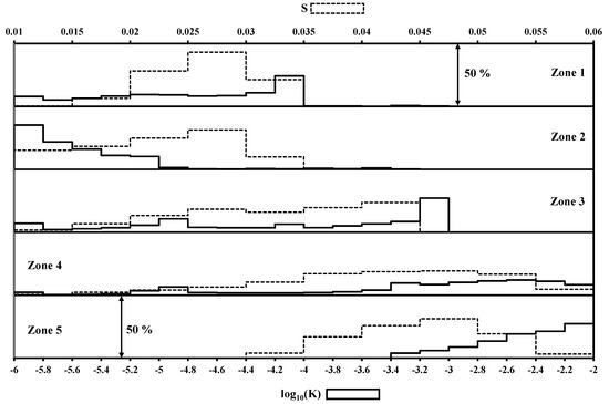
Figure 7.
Zonal parameter distribution for the set of 158 solutions (solid histograms: hydraulic conductivity, dashed histograms: specific yield).
The same pattern occurred with the soil water storage capacity in zones 1, 2, and 3 (see Table 6). However, the parameter bounds were not allowed lower for the sake of realism nor higher considering the industrial use of this part of the site. However, the SW influence on recharge was overtaken by the high level of soil sealing (high runoff ratio) in these zones.
4.3. Piezometry and Water Balance
In order to further analyze the consistency of the calibration, the difference between computed and measured heads was estimated for each piezometer k (Figure 8), using the average error (AE) and standard deviation error (SE) defined as:
where Nt is the number of piezometric heads measured at well k, Ns is the number of solutions, is the estimated water head at well k for solution j, and is the corresponding ith measured value.
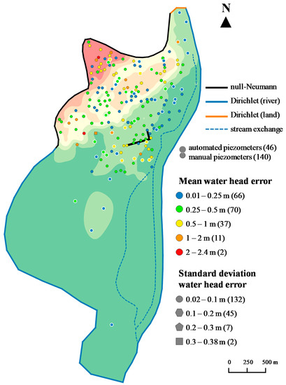
Figure 8.
Mean and standard deviation of water head error for the set of solutions.
Overall, the optimization was quite robust since the SEs were quite low (less than 10 cm for most piezometers). No spatial trends appeared in the distribution of AE and SE; however, the upper terrace showed the highest discrepancy due to a very complex piezometric context (strong gradients in several directions). High AE also impacted control points located on terrace transitions, where the two-dimensional approach was less relevant. On the other hand, small AE and SE occurred near prescribed head boundaries.
Results for one solution are reported in Figure 9 in order to visualize the different piezometric behaviors in the study area and their corresponding calibration. Although the number of continuous data was very scarce in the upper terrace, the inversion succeeded in producing the sharp fluctuations (P1) expected in this zone. The middle terrace ridge piezometric pattern (P2) is poorly documented. Therefore, the calibration in this zone was focused on reproducing the piezometric dome rather than the water head fluctuations to ensure realistic groundwater flow directions. As a result, water levels in the rest of the middle terrace (e.g., P3, P4) are quite satisfactorily simulated. Concerning the lower terrace and the alluvial plain, the calibration confirms the chosen boundary conditions and of the recharge model. In the agricultural part of the site, even far from the rivers (P8), groundwater base level and fluctuations are very well reproduced. On the other hand, P7 is shown as an example of offset calibration, with a shifted base level but consistent fluctuations. It is assumed that a local lack of accuracy in boundary conditions discretization or the stream exchange term could be the cause of this kind of error.
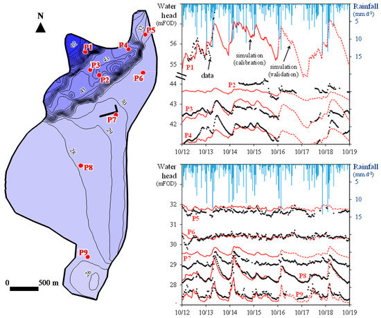
Figure 9.
Piezometric map and some fits for a sample solution.
On the grounds of simulation results during the verification period, the model’s parametrization was found to be very robust, especially as years 2017 and 2018 were meteorological extremes, with, respectively, 332 and 1100 mm of yearly rainfall (compared to 533, 787, 956, 791, and 761 mm during the calibration period). These conditions have particularly strong implications in the zones where precipitation is the only input for recharge (upper and middle terraces) and considering the limitations of the 2D approach in a context with important vertical gradients (terrace transitions). For the shown sample solution, the overall simulation error in the verification period maintained the same level of accuracy as the calibration period for the automated piezometers (mean error of 0.34 m).
The example solution’s water balance is reported in Table 7. Dirichlet boundary conditions (mostly head prescribed rivers) were the main water input of the model as expected in an alluvial context. Recharge from precipitation yielded up to 20% of the total rainfall with loss driven by soil sealing in the industrial part of the site and by evapotranspiration in the agricultural plain. Stream–aquifer exchange acted as drainage, consistent with field observations, but its rate was still uncalibrated. Finally, the numerical error (estimated by the discrepancy between the stock variation and the inflow/outflow balance) remained very low, attesting that the discretization and the computation of the transmissivity were accurate.
Table 7.
Global water balance of the sample solution (in 104 m3) over the 286 computed decadal time steps.
5. Conclusions
An adjoint state-based inversion procedure, coupled with a Zoned Adaptive Multiscale Triangulation (ZAMT) parametrization, was developed to estimate groundwater flow parameter distribution. This novel parametrization scheme combines the strengths of AMT (flexibility in the parameter distribution) and zonation (integration of distributed a priori information on a large scale). Each ZAMT vertex can be associated with an independent parameter range, narrowing down the space of solutions consistent with “soft” geological data.
The inverse problem’s objective function, based on generalized weighted least squares, integrates an original regularization term χ, penalizing the function value when computed water heads are outside realistic limits. This plausibility criterion adds a constraint for the piezometry on the whole domain, which is particularly beneficial when water head measurements are scarce. Moreover, it allows to better handle shallow aquifers (where computation is likely to conflict with the ground surface level) and thin saturated zones (conflicts with the substratum level), especially with steep topographic gradients.
Parameter estimation based on water heads only is a difficult task because of a lack of sensitivity of the parameters to the variable. Therefore, the ensemble of possible solutions is in general very large. Adding information by (i) including an additional term in the objective function, and (ii) constraining the parameter over the domain through the ZAMT methodology reduces the number of possible solutions.
The study case is a phreatic alluvial aquifer of 6.64 km² located in the south of France with strong variations in topography and metric saturated thickness. With respect to the terraced organization of the site, the ZAMT was used to distinguish 5 zones, the higher and older terraces’ geological material being less permeable than the lower ones. The χ plausibility criterion was activated with the substratum and ground level as limits to better constrain the simulation in areas with steep topography (terrace transitions, cuesta), very shallow water levels, and/or thin saturated thicknesses. The simulations were calibrated with 5 years of data (2012–2016) and the quality of the calibration was verified over 3 years (2017–2019) at a decadal time step with 191 control points.
The χ criterion produces better parametrization, resulting in lower water head discrepancies (a set of 150 solutions yields a mean error of 0.43 m with the criterion, 0.55 m without it) and more realistic piezometric fields. Notably, it has allowed better water head constraint on the substratum ridge (zone 2), which lacks piezometric data but largely conditions the flow direction for an important part of the model. The ZAMT kept the parameter (hydraulic conductivity and specific yields) in ranges consistent with the geological nature of the aquifer.
An adjusting threshold of 0.40 m (mean error between measured and simulated water head) was found adequate to filter 500 model calibrations, resulting in a set of 153 satisfactory solutions. The set of solutions shows very stable parameter fields.
Concerning the water head calibration, the best fits were obtained near the river boundaries and in the lower plain (southern and eastern fringes), while greater discrepancy and variability were noted in the upper terraces of the site (northwest), where steep local topographic gradients of the aquifer substratum challenges the inversion procedure and the model assumptions (horizontal flow). Nevertheless, even in these areas where water is only supplied by rainfall, the parametrization is found to be robust, maintaining realistic levels in a particularly dry context (year 2017).
Concerning the shallowness of the aquifer and the quick piezometric response attested by the control data chronicles, the recharge parameters (Nash) displayed a very low level of influence. Moreover, the recharge model’s non-linear response to the decadal time discretization was successfully handled and produced heterogeneous piezometric behaviors consistent with the measurements. The total volume of recharge over the period represented 20% of the rainfall and contributed to a global water balance with very marginal numerical loss. The simulated surface water bodies’ behavior was coherent with the expectations: the bordering rivers were suppliers upstream, outlets downstream, and the in-site streams drained the aquifer.
Although the assumption of independence was made, the model could benefit from a denser piezometer network in the northeastern part of the site and beyond the actual boundary in order to determine to which extent the neighboring geological domain is connected to the alluvial aquifer. Moreover, the current model runs with uncalibrated and undiscretized stream–aquifer exchange rates. A field survey relative to this matter is a crucial need to enhance the model accuracy in its lower part.
Author Contributions
Conceptualization, D.R. and P.A.; Formal analysis, P.A. and O.B.; Investigation, O.B.; Methodology, D.R.; Project administration, O.B.; Supervision, P.A. and O.B.; Validation, D.R.; Writing—original draft, D.R.; Writing—review & editing, P.A. and O.B. All authors have read and agreed to the published version of the manuscript.
Funding
This research received no external funding.
Acknowledgments
This study has been funded by the MRISQ project at the CEA. We thank the three anonymous reviewers whose comments were very helpful in improving the manuscript.
Conflicts of Interest
The authors declare no conflict of interest.
References
- Carrera, J.; Neuman, S.P. Estimation of aquifer parameters under transient and steady state conditions: 1. maximum likelihood method incorporating prior information. Water Resour. Res. 1986, 22, 199–210. [Google Scholar] [CrossRef]
- Poeter, E.P.; Hill, M.C. Inverse models: A necessary next step in groundwater modeling. Ground Water 1997, 35, 250–260. [Google Scholar] [CrossRef]
- Yakowitz, S.; Duckstein, L. Instability in aquifer identification: Theory and case studies. Water Resour. Res. 1980, 16, 1045–1064. [Google Scholar] [CrossRef]
- McLaughlin, D.; Townley, L.R. A reassessment of the groundwater inverse problem. Water Resour. Res. 1996, 32, 1131–1161. [Google Scholar] [CrossRef]
- Hadamar, J. Le Problème de Cauchy et les Équations aux Dérivées Partielles Linéaires Hyperboliques; Herman: Paris, France, 1932. [Google Scholar]
- Sun, N.-Z.; Yeh, W.W.-G. Identification of parameter structure in groundwater inverse problem. Water Resour. Res. 1985, 21, 869–883. [Google Scholar] [CrossRef]
- Carrera, J.; Alcolea, A.; Medina, A.; Hidalgo, J.; Slooten, L.J. Inverse problem in hydrogeology. Hydrogeol. J. 2005, 13, 206–222. [Google Scholar] [CrossRef]
- Coats, K.H.; Dempsey, J.R.; Henderson, J.H. A new technique for determining reservoir description from field performance data. Soc. Pet. Eng. J. 1970, 10, 66–74. [Google Scholar] [CrossRef]
- Yoon, Y.S.; Yeh, W.W.-G. Parameter identification in an inhomogeneous medium with the finite-element method. Soc. Pet. Eng. J. 1976, 16, 217–226. [Google Scholar] [CrossRef]
- Garay, H.L.; Haimes, Y.Y.; Das, P. Distributed parameter identification of groundwater systems by nonlinear estimation. J. Hydrol. 1976, 30, 47–61. [Google Scholar] [CrossRef]
- Certes, C.; de Marsily, G. Application of the pilot point method to the identification of aquifer transmissivities. Adv. Water Resour. 1991, 14, 284–300. [Google Scholar] [CrossRef]
- Tsai, F.T.-C.; Yeh, W.W.-G. Characterization and identification of aquifer heterogeneity with generalized parametrization and Bayesian estimation. Water Resour. Res. 2004, 40. [Google Scholar] [CrossRef]
- Hendricks Franssen, H.J.; Alcolea, A.; Riva, M.; Bakr, M.; van der Wiel, N.; Stauffer, F.; Guadagnini, A. A comparison of seven methods for the inverse modelling of groundwater flow: Application to the characterisation of well watchments. Adv. Water Resour. 2009, 32, 851–872. [Google Scholar] [CrossRef]
- Yeh, W.W.-G.; Yoon, Y.S. Aquifer parameter identification with optimum dimension in parametrization. Water Resour. Res. 1981, 17, 664–672. [Google Scholar] [CrossRef]
- Eppstein, M.J.; Dougherty, D.E. Simultaneous estimation of transmissivity values and zonation. Water Resour. Res. 1996, 32, 3321–3336. [Google Scholar] [CrossRef]
- Sun, N.-Z.; Yang, S.-L.; Yeh, W.W.-G. A proposed stepwise regression method for model structure identification. Water Resour. Res. 1998, 34, 2561–2572. [Google Scholar] [CrossRef]
- Lu, Z.; Robinson, B.A. Parameter identification using the level set method. Geophys. Res. Lett. 2006, 33. [Google Scholar] [CrossRef]
- Lien, M.; Berre, I.; Mannseth, T. Combined adaptive multiscale and level-set parameter estimation. Multiscale Model. Simul. 2006, 4, 1349–1372. [Google Scholar] [CrossRef]
- Cardiff, M.; Kitanidis, P.K. Bayesian inversion for facies detection: An extensible level set framework. Water Resour. Res. 2009, 45. [Google Scholar] [CrossRef]
- Majdalani, S.; Ackerer, P. Identification of groundwater parameters using an adaptive multiscale method. Ground Water 2011, 49, 548–559. [Google Scholar] [CrossRef]
- Ackerer, P.; Trottier, N.; Delay, D. Flow in double-porosity aquifers: Parameter estimation using an adaptive multiscale method. Adv. Water Resour. 2014, 73, 108–122. [Google Scholar] [CrossRef]
- Hassane, M.M.; Ackerer, P. Groundwater flow parameter estimation using refinement and coarsening indicators for adaptive downscaling parameterization. Adv. Water Resour. 2017, 100, 139–152. [Google Scholar] [CrossRef]
- McDonald, M.G.; Harbaugh, A.W. A Modular Three-Dimensional Finite-Difference Ground-Water Flow Model; USGS: Washington, DC, USA, 1988. [Google Scholar]
- Crouzeix, M.; Raviart, P.-A. Conforming and nonconforming finite element methods for solving the stationary Stokes equations. Revue Française d’Automatique, Informatique, Recherche Opérationnelle. Mathématique 1973, 7, 33–75. [Google Scholar] [CrossRef]
- Simmers, I. Estimation of Natural Groundwater Recharge; Springer: Dordrecht, The Netherlands, 1987. [Google Scholar]
- Richards, L. Capillary conduction of liquids through porous mediums. Physics 1931, 1, 318–333. [Google Scholar] [CrossRef]
- Brooks, R.H.; Corey, A.T. Hydraulic Properties of Porous Media; Colorado State University: Fort Collins, CO, USA, 1964. [Google Scholar]
- Mualem, Y. A new model for predicting the hydraulic conductivity of unsaturated porous media. Water Resour. Res. 1976, 12, 513–522. [Google Scholar] [CrossRef]
- Besbes, M.; De Marsily, G. From infiltration to recharge: Use of a parametric transfer function. J. Hydrol. 1984, 74, 271–293. [Google Scholar] [CrossRef]
- Tarantola, A. Inverse Problem Theory and Methods for Model Parameter Estimation; Society for Industrial and Applied Mathematics: Philadelphia, PA, USA, 2005. [Google Scholar]
- Neuman, S.P. Generalized scaling of permeabilities: Validation and effect of support scale. Geophys. Res. Lett. 1994, 21, 349–352. [Google Scholar] [CrossRef]
- Sánchez-Vila, X.; Carrera, J.; Girardi, J.P. Scale effects in transmissivity. J. Hydrol. 1996, 183, 1–22. [Google Scholar] [CrossRef]
- Kitanidis, P.K.; Lane, R.W. Maximum likelihood parameter estimation of hydrologic spatial processes by the Gauss-Newton method. J. Hydrol. 1985, 79, 53–71. [Google Scholar] [CrossRef]
- Carter, R.D.; Jemp, L.F.J.; Pierce, A.C.; Williams, D.L. Performance matching with constraints. Soc. Pet. Eng. J. 1974, 14, 187–196. [Google Scholar] [CrossRef]
- Byrd, R.H.; Lu, P.; Nocedal, J.; Zhu, C. A limited memory algorithm for bound constrained optimization. J. Sci. Comput. 1995, 16, 1190–1208. [Google Scholar] [CrossRef]
- Townley, L.R.; Wilson, J.L. Computationally efficient algorithms for parameter estimation and uncertainty propagation in numerical models of groundwater flow. Water Resour. Res. 1985, 21, 1851–1860. [Google Scholar] [CrossRef]
- Pebesma, E.J.; Heuvelink, G.B.M. Latin Hypercube Sampling of Gaussian Random Fields. Technometrics 1999, 41, 303–312. [Google Scholar] [CrossRef]
- Rajabi, M.M.; Ataie-Ashtiani, B.; Janssen, H. Efficiency enhancement of optimized Latin hypercube sampling strategies: Application to Monte Carlo uncertainty analysis and meta-modeling. Adv. Water Resour. 2015, 76, 127–139. [Google Scholar] [CrossRef]
- Turc, L. Evaluation des besoins en eau d’irrigation, évapotranspiration potentielle. Ann. Agron. 1961, 12, 13–49. [Google Scholar]
© 2020 by the authors. Licensee MDPI, Basel, Switzerland. This article is an open access article distributed under the terms and conditions of the Creative Commons Attribution (CC BY) license (http://creativecommons.org/licenses/by/4.0/).