An Improved Meshless Divergence-Free PBF Framework for Ocean Wave Modeling in Marine Simulator

Abstract

It is a challenging work to simulate wind and waves in virtual scenes of marine simulators. In this paper, a divergence-free position based fluid (DFPBF) framework is introduced for ocean wave modeling in marine simulators. We introduce a set of constant density constraints and divergence-free velocity constraints to enforce incompressibility. By adjusting the position distribution of fluid particles, the particle density is forced to be constant. Constraining the divergence-free velocity field can keep the density change rate at zero. When correcting the position and velocity of particles, we introduced a relaxation correction scheme to accelerate the convergence of the framework. The simulation results show that as the scene scale expands and the number of fluid particles increases, this acceleration effect will be more significant. Secondly, we propose a novel particle-based three-dimensional stochastic fluctuating wind field. The Perlin noise is introduced to disturb the constant horizontal wind field to form a stochastic wind field. On this basis, a stochastic fluctuating wind field simulation framework is proposed. By adjusting the pulse period and pulse width, users can flexibly control the fluid turnover under the action of the wind field. This wind field framework can be easily integrated into the DFPBF model. Based on this wind field model, we simulated some typical wind wave scenarios, including interaction scenarios with lighthouse and lifebuoy, and verified the effectiveness of the wind field model.

1. Introduction

1.1. Motivation

Particle-based fluid simulation is a challenging subject in computer graphics. The realistic simulation of the dynamic evolution of fluid scenes has great applications in the areas such as defense industry, transportation training, disaster prevention, rescue training, games development, film special effects, and computer animation. The visual system of a marine simulator is one of the important engineering applications. Marine simulators have been widely applied to fields of marine education and training, engineering demonstration, and scientific research, etc. The International Convention on Standards of Training, Certification and Watchkeeping for Seafarers and its amendments put forward a series of mandatory requirements and suggestions on the performance standards, scope of application, and rules of the use of marine simulators. Improving the performance of marine simulators is required by both international conventions and nautical practices. The visual system is the most direct and the largest source of information for simulator operators, and is also an important part of marine simulators and one of the important indexes to evaluate the performance of marine simulators. Wind and waves are one of the typical fluid scenes, in marine simulators, which can be used to train the officer’s ship-handling skills in wind waves, and it can also be used for engineering demonstrations such as testing the strength of ships, offshore structures, breakwaters, and other structures. In nautical practices, extreme weather is extremely dangerous, sometimes with disastrous consequences. The handling capacity of the ship’s officer is closely related to the ship’s safety in extreme weather such as heavy sea. This kind of handling capabilities require a lot of training, but training in a real environment is almost impossible, and there is a great risk of personal injury and property damage. Therefore, marine simulator training has become an effective alternative. Through the realistic simulation of extreme weather, the zero-risk training of ship handling under the environment of heavy wind and waves can be realized, which has a very good preventive effect on the disastrous consequences.

In the existing marine simulators, the simulation of wind waves is mainly based on spectrum-based approaches. The spectrum-based approaches rely on the height field grids, so when simulating splash scenes, they need to be coupled with other models. In order to simplify the modeling of splash scenes in marine simulators and enhance physical reality, we tried to introduce the meshless particle method in marine simulators. At the same time, in order to make the marine simulator better applied to train the emergency maneuverability of the crew in extreme weather conditions, we aim to propose a novel wind field model for the meshless framework to simulate the sea conditions under extreme weather. Our research aims to provide some feasible solutions for the development and performance improvement of marine simulators, and to provide technical support for ensuring the safety of marine traffic.

1.2. Related Work

1.2.1. Spectrum-Based Approaches

The spectrum-based approaches treat ocean waves as consisting of an infinite number of individual waves with different amplitudes, different frequencies, different directions, and random phases. Wave spectrum describes the distribution of wave energy relative to individual waves. Generally, the wave spectrum contains wind parameters. By adjusting the wind direction and wind speed, the wind wave scene can be simulated realistically. Tessendorf [1] introduced the spectrum method into computer graphics. He used the Phillips spectrum as the wind wave motion model, which is still the main solution of wind wave simulation in the industrial field until now. The Phillips spectrum contains wind speed $V$ and wind direction $\widehat{\omega }$, and it can generate waves with different amplitudes according to a given wind speed and wind direction. Other wave spectrums commonly used in wind wave simulation also includes Pierson-Moskowitz (PM) spectrum [2,3], Joint North Sea Wave Observation Project (JONSWAP) spectrum [4,5], and Texel MARSEN ARSLOE (TMA) spectrum [6,7], etc. The PM spectrum is suitable for simulating fully developed seas and the JONSWAP spectrum is suitable for simulating the continued development of waves in deep water. The JONSWAP spectrum is obtained by multiplying an extra peak enhancement factor $\gamma$ on the basis of the PM spectrum. Therefore, compared to the PM spectrum, its spectral shape is more concentrated near the peak and more sharper. The TMA spectrum is the product of the JONSWAP spectrum and the Kitaigorodskii Depth Attenuation function [8,9], and the TMA spectrum extends the application of the JONSWAP spectrum to shallow water areas. The spectrums mentioned above are all frequency spectrums $S\left(\omega \right)$, whereas directional spectrums $S\left(\omega ,\theta \right)$ are the extension of frequency spectrums, which add directional information $D\left(\omega ,\theta \right)$ on the basis of frequency spectrums. The wave number spectrum $\Psi \left(k\right)$ can be obtained by changing the angular frequency $\omega$ of individual waves into a wave number $k$.

The spectrum-based approaches based on fast Fourier transform are suitable for parallel acceleration, and the calculation speed is fast. With the whitecap model [10], they can simulate realistic ocean scenes. Therefore, they have been widely used. However, there are some limitations in the spectrum-based approaches. They are difficult to simulate the wave breaking effect due to the limitation of the height field grid. Generally, separate modeling is needed for the wave breaking effect, resulting in complicated hybrid models. In heavy wind and wave weather, the undulations of the waves change drastically, and special scenes such as overturns, breaks, and green water often appear, which is difficult to simulate using spectrum-based approaches.

1.2.2. Physics-Based Methods

The physics-based method mainly uses Navier-Stokes Equations (NSE) to model fluid motion. According to the different methods of solving NSE, it can be divided into the Eularian method and the Lagrangian method. Eularian method [11] is a grid-based method [12]. Although physics-based modeling has greatly increased the physical accuracy of the model, it also has many limitations when simulating large deformation scenes such as overturns and breaks. Therefore, many researchers use the Lagrangian method to simulate large deformation scenes of ocean waves. The Lagrangian method is a particle-based method. It analyzes the movements of individual particles in a fluid, studies the changes in the velocity, pressure, density and other parameters of a given particle in a fluid over time, and studies the changes of parameters when changing from one fluid particle to another fluid particle. In computer graphics, the most commonly used Lagrangian method is the smoothed particle hydrodynamics (SPH) method [13,14,15]. In the SPH method, the physical quantities of fluid particles come from the interpolation of the corresponding physical quantities of other particles in the support domain. The SPH method does not need to layout a grid in the problem domain, so it is not limited by the grid. It also has significant advantages in dealing with large deformation scenes and geometrically complex boundary interaction problems. The SPH method was first introduced into computer graphics by Stam [16] to simulate fire, smoke, and other gaseous phenomena. Then, Müller [17] simulated the interactive fluid scenes based on the SPH method for the first time in computer graphics. However, limited by the hardware conditions at that time, the range of fluid scenes is small. Moreover, the incompressibility of the SPH model based on the ideal gas equation of state (EOS) is poor. Subsequently, in computer graphics, most of the SPH literatures focus on the optimization of pressure term to enhance the incompressibility of the model. The study of incompressibility is mainly focused on the treatment of pressure items. In the fluid simulation for computer graphics, there are usually two schemes to deal with the pressure term: the EOS-based methods and the PPE-based (Pressure Poisson equation) methods. Typical EOS-based methods include WCSPH (Weakly Compressible SPH) [18,19], PCISPH (Predictive-Corrective Incompressible SPH) [20], and LPSPH (Local Poisson SPH) [21]. Among them, PCISPH and LPSPH use a pressure projection scheme, and update pressure iteratively. They allow larger time steps than the WCSPH, which is based on Tait equation. Typical PPE-based methods include ISPH (Incompressible SPH) [22,23], IISPH (Implicit Incompressible SPH) [24], and DFSPH (Divergence-Free SPH) [25]. The main difference between the PPE-based methods is the source item of PPE. There are currently three common source items: density invariance [24], velocity divergence [25], and particle shift [26]. Compared with the EOS-based method, the PPE-based method has a larger time step and better incompressibility. In fact, EOS-based and PPE-based pressure solving methods are both force-based methods, which update particle velocity through pressure acceleration. Müller et al. [27] proposed a position-based dynamic (PBD) framework that immediately works on the particle positions. Macklin and Müller [28] introduced the density constraints [29] into the PBD framework and named it position-based fluid (PBF). PBF is a very attractive real-time fluid simulation method that allows large time steps and is very stable, and it was adopted by Nvidia’s physical engine, FleX, which has been widely used in various virtual reality scenarios. Based on the concept of PBF, Kang and Sagong [30] added a set of divergence-free velocity field constraints, called FISPH (Fully Incompressible SPH), but compared with the PBF method, the FISPH method has no obvious speed advantage.

Wind is the motion of air. In aerodynamics, air can be regarded as a Newtonian fluid. Therefore, wind waves are the interactive movement between the two-phase fluids of air and ocean. In the SPH framework, the ideal way is to model the wind waves using the multiphase flow model, but due to the high density ratio, it usually causes stability problems. Moreover, the number of air particles sampled is huge, and the computation is very expensive. Due to the above problems, some researchers try to sample air particles only in the interaction area to save computing resources [31,32]. However, these solutions are relatively complicated when managing air particles, so some single-phase solutions [33,34,35] based on drag forces have been proposed, which improves the interaction between air and fluid. The modeling research of high-speed wind field in the SPH framework is still few in computer graphics.

The SPH method also has many applications in simulating certain scale ocean scenes, preferably the wind wave scenes. Akinci et al. [36] proposed a momentum-conserving two-way fluid-rigid coupling model of SPH fluids, and simulated the scene of a frigate sailing on wavy sea, which is still a state-of-the-art fluid-solid coupling method up to now. Macklin and Müller [28] simulated the real-time interaction between ocean waves and lighthouse based on the PBF framework. Ihmsen et al. [24] simulated the scene of a cargo ship in highly agitated ocean using the IISPH method. Bender et al. [37] proposed a micropolar material model to simulate the turbulent inviscid fluids. They simulated the interaction between ocean and a fast-rotating propeller, and the scenario of a turbulent river flowing through a complex river course. The micropolar fluid method solves the problem of turbulence detail loss caused by the numerical dissipation of the SPH model, and is linear and angular momentum conserving. They then proposed a post-processing model on the basis of the micropolar fluid model to simulate realistic foam effects [38]. Losasso et al. [39] proposed a hybrid method that used the particle level set method to model dense liquid volumes and a SPH method to simulate diffuse regions. A large ocean scene with fine-detail mist and foam was simulated using the coupling method.

1.3. Our Contributions

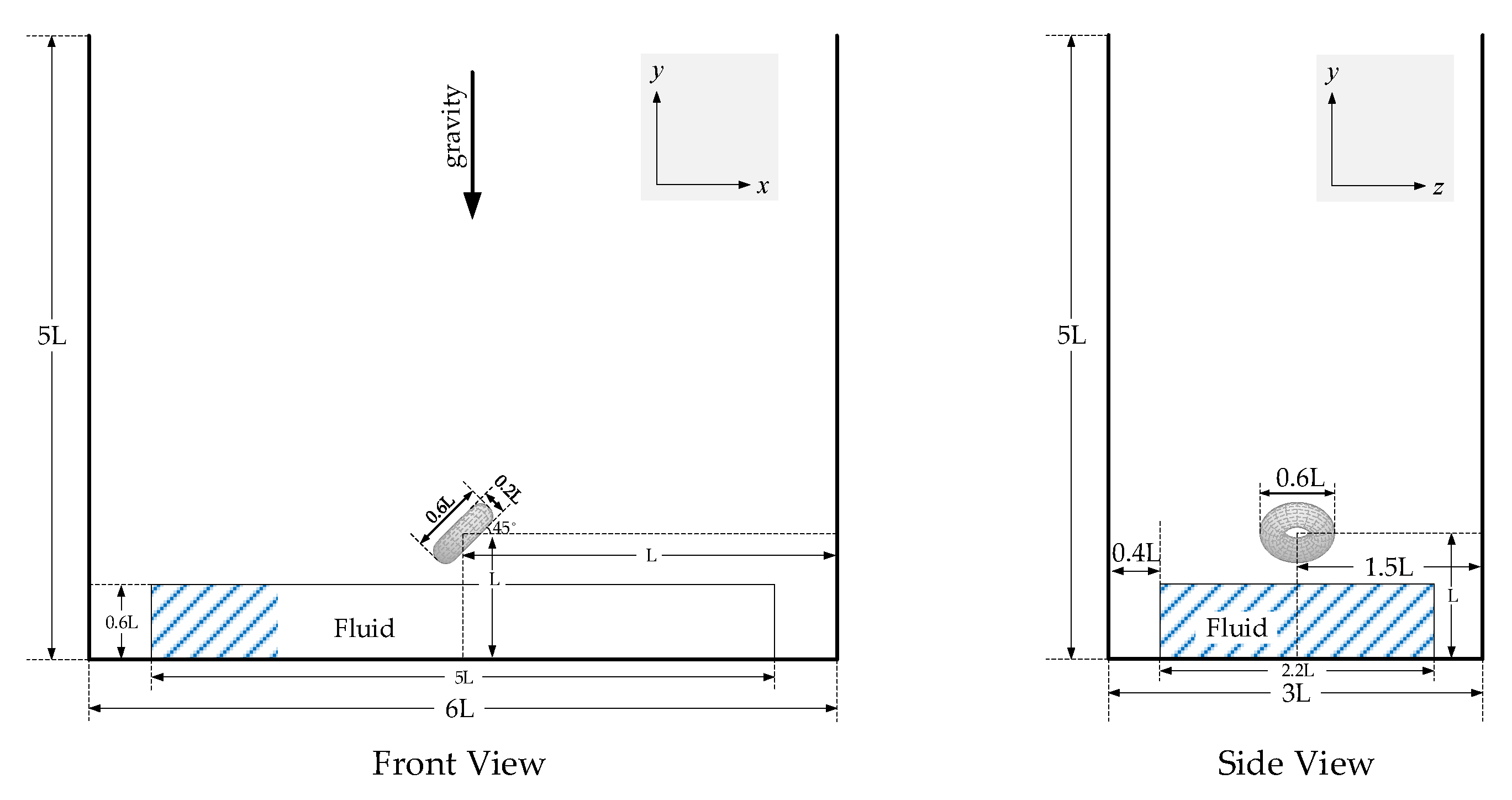
In order to solve the limitation of the spectrum-based approaches in simulating splash scenes and increase the physical realism of the ocean scene in marine simulators, we propose an improved divergence-free PBF (DFPBF) framework. We introduce a series of constant density constraints and divergence-free velocity field constraints to satisfy the incompressibility of the ocean in marine simulators. The positional density constraints directly adjust the particle distribution by solving the position correction to keep the density level constant. Inspired by the concept of PBF, we introduce a set of improved divergence-free velocity field constraint to keep the density change rate at zero. In iterative calculation, we introduce a user-defined relaxation factor, which greatly accelerates the convergence of the algorithm.

In order to make the marine simulator meet the training needs of the crew’s emergency maneuvering ability in extreme weather scenarios, we desired to simulate the ocean free surface under the action of wind fields based on the DFPBF framework. Therefore, we propose a novel three-dimensional wind field empirical model, which can be easily integrated into our DFPBF method. By adding Perlin noise, the wind field model can generate realistic stochastic wind fields. Under the action of stochastic wind fields, the ocean surface will produce the effect of waves overturning, which further enriches the details of the ocean scene in the visual system of marine simulators. On this basis, we propose a novel wind wave simulation framework based on the DFPBF model. By adjusting the pulse period and pulse width, we can flexibly control the fluid turnover under the action of wind field.

2. Fluid Simulation

2.1. Governing Equations

In physics-based methods, the velocity fields $v$, pressure fields $p$, density fields $\rho$, temperature fields $T$, and salinity fields $s$ are usually used to describe the moving and changing oceans. The basic laws of physics that play a dominant role in the movement of ocean waves are the law of conservation of mass, the law of conservation of momentum, and the law of conservation of energy. Here, we assume that the ocean is a homogeneous incompressible fluid with a constant temperature, so the effects of temperature and salinity changes are not considered, that is, energy changes need not be considered. Therefore, we use the Navier-Stokes equations as the governing equation of ocean wave motion:

$$\frac{D\rho }{\mathit{Dt}}+\rho \nabla \cdot v=0,$$

(1)

$$\rho \frac{Dv}{\mathit{Dt}}=-\nabla p+\mu {\nabla }^{2}v+f,$$

(2)

where $\rho$ is the density, $t$ is the time, $v$ is the velocity, $p$ is the pressure, $\mu$ is the dynamic viscosity, and $f$ is the external force acting on unit fluid element, and in this paper, only the gravity is considered. $Dv/\mathit{Dt}$ is the substantial derivative of velocity, which tracks the time rate of change of the velocity of a moving unit fluid element. $\nabla$ is the hamiltonian operator, and $\nabla =\frac{\partial }{\partial x}i+\frac{\partial }{\partial y}j+\frac{\partial }{\partial z}k$. ${\nabla }^2=\nabla ·\nabla$ is the laplacian operator, and ${\nabla }^2=\frac{{\partial }^2}{\partial x^2}+\frac{{\partial }^2}{\partial y^2}+\frac{{\partial }^2}{\partial z^2}$.

In the incompressible framework, the density can be assumed by the rest density ${\rho }_0$, so the governing equation can be transformed into:

$$\nabla \cdot v=0,$$

(3)

$${\rho }_0\frac{Dv}{\mathit{Dt}}=-\nabla p+\mu {\nabla }^{2}v+f$$

(4)

2.2. Discretization of the Continuum Domain

In PBF method, the density is discretized as follows:

$${\rho }_i={{\displaystyle \sum }}_j{m}_j{W}_{\mathit{ij}}={\rho }_0{{\displaystyle \sum }}_j{V}_j{W}_{\mathit{ij}},$$

(5)

where ${\rho }_i$ is the density of particle $i$,$m_j$ is the mass of the neighboring particle, ${\rho }_0$ is the rest density, and $V_j$ is the volume of the neighboring particle. We assumed that all particles in the neighborhood of $i$ have the rest density and volume of particle $i$. $W_{\mathit{ij}}$ is a smoothing kernel function and $W_{\mathit{ij}}=W\left(x_i-x_j, h\right)$, $h$ is the support radius, $x_i$ denotes the position of particle $i$, and $x_j$ is the position of the neighboring particle.

The difference between the PBF method and the SPH method lies in their different way of solving pressure terms. In the PBF method, the pressure gradient is achieved through density constraints, and the positions of the particles are directly updated. We will discuss density constraints in detail in the following sections. There are many methods to calculate the viscosity term $\mu {\nabla }^{2}v$. Here we use the artificial viscosity [40,41,42]:

$${\nabla }^2{v}_i=2\left(d+2\right){\rho }_0{{\displaystyle \sum }}_j\frac{V_j}{{\rho }_j}{v}_{\mathit{ij}}\frac{x_{\mathit{ij}}·\nabla W_{\mathit{ij}}}{x_{\mathit{ij}}·x_{\mathit{ij}}+0.01h^2},$$

(6)

where $v_{\mathit{ij}}=v_i-v_j$, $x_{\mathit{ij}}=x_i-x_j$, $d$ is the number of spatial dimensions, and term $0.01h^2$ is introduced in the denominator to avoid singularities. $\nabla W_{\mathit{ij}}={\left(\partial W_{\mathit{ij}}/\partial x_{i,x},\partial W_{\mathit{ij}}/\partial x_{i,y},\partial W_{\mathit{ij}}/\partial x_{i,z}\right)}^T$.

2.3. Constant Density Constraints

In the PBF method, pressure is achieved through density constraints. By solving the density constraints, a particle position correction can be obtained for directly adjusting the particle position distribution. A uniform particle distribution can keep the density stable at the rest density level.

$$C_i=\frac{{\rho }_i}{{\rho }_0}-1\le 0,$$

(7)

Each constraint $C_i$ is a function of the particle’s position and the positions of its neighbors. Obviously, the form of Equation (7) is very similar to the Tait equation in Becker’s work 19, except that the stiffness parameters $B$ and $\gamma$ in the Tait equation are set to 1 here. In the PBF method, the density estimation in Equation (5) is more accurate only when there are sufficient neighboring particles. However, in the free surface area, the number of neighboring particles is generally insufficient, so the density constraints based on Equation (7) will cause particle clustering or clumping. Macklin [28] added an artificial pressure to alleviate this problem. Considering the computational efficiency, we used inequality constraints to achieve similar effects, that is, only the regions with larger particle density estimates are corrected. According to Equation (7), the distribution of fluid particles should satisfy $C_i\left(x+∆x\right)\le 0$, which can be expanded in a Taylor series, and the final position correction $∆x_i$ for particle $i$ is:

$$∆x_i={\lambda }_i\nabla C_i,$$

(8)

where $\nabla C_i$ is the constraint gradient in Equation (7). ${\lambda }_i$ is the scaling factor:

$${\lambda }_i=-\frac{C_i}{\nabla C_i·\nabla C_i},$$

(9)

$\nabla C_i$ has two different cases based on whether $k$ in the following equation is a neighboring particle or not:

$${\nabla }_k{C}_i=\{\begin{array}{c}{{\displaystyle \sum }}_j{V}_j{\nabla }_k{W}_{\mathit{ij}}, \mathrm{if} k=i\\ -V_j{\nabla }_k{W}_{\mathit{ij}}, \mathrm{if} k=j\end{array},$$

(10)

Inserting Equation (10) into Equation (9):

$${\lambda }_i=C_i{\alpha }_i,$$

(11)

where ${\alpha }_i=-1/\left(|{{\displaystyle \sum }}_j{V}_j\nabla W_{\mathit{ij}}{|}^2+{{\displaystyle \sum }}_j|V_j\nabla W_{\mathit{ij}}{|}^2\right)$.

The position correction of the particle $i$ under the density constraints can be derived as:

$$∆x_i={\lambda }_i\nabla C_i={\lambda }_i{\nabla }_i{C}_i+{{\displaystyle \sum }}_j{\lambda }_j{\nabla }_j{C}_j={{\displaystyle \sum }}_j{V}_j\left({\lambda }_i+{\lambda }_j\right)\nabla W_{\mathit{ij}},$$

(12)

The position of fluid particles is corrected by $∆x_i$, so that the distribution of fluid particles satisfies the density constraints. This is different from the traditional force-based methods, which do not need to adjust the position of particles through the velocity. Relatively speaking, position based correction is more efficient. When correcting the particle position, a relaxation factor is introduced, which can artificially accelerate the particle position correction process in the gradient direction, thereby accelerating convergence:

$$x_i=\left(x_i+∆x_i\right)+\omega ∆x_i=x_i+\left(1+\omega \right)∆x_i,$$

(13)

where $\omega$ is a user-defined relaxation factor, in our relaxation correction scheme, $\omega =0.1$. We describe the calculation flow of the constant density solver in detail in Appendix A.

2.4. Divergence-Free Velocity Constraints

Inspired by the work of Asai et al. [23] and Kang and Sagong [30], we introduced modified divergence-free velocity constraints in the ocean modeling of the marine simulator. The divergence-free velocity constraints can be expressed as:

$$C_i^v=\nabla ·v_i={{\displaystyle \sum }}_j{V}_j{v}_{\mathit{ij}}·\nabla W_{\mathit{ij}}\le 0,$$

(14)

In the derivation, we found that the rest density ${\rho }_0$ can be reduced, so here we adopted the divergence-free velocity constraints in Equation (14). Considering the same reason as Equation (7), we also used inequality constraints here. According to Equation (14), the velocity divergence of fluid particles should satisfy $C_i^v\left(v+∆v\right)\le 0$, which can also be expanded in a Taylor series:

$$C_i^v\left(v+∆v\right)=C_i^v\left(v\right)+{\nabla }_v{C}_i^v\left(v\right)∆v_i,$$

(15)

Since the constraint $C_i^v$ is minimized maximally along its gradient direction, so we assumed that the velocity changes along the gradient direction:

$$∆v_i={\lambda }_i^v{\nabla }_{v_i}{C}_i^v\left(v\right),$$

(16)

Substituting Equation (16) into Equation (15), we can get:

$${\lambda }_i^v=\frac{C_i^v\left(v\right)}{{\nabla }_{v_i}{C}_i^v\left(v\right)·{\nabla }_{v_i}{C}_i^v\left(v\right)},$$

(17)

And the gradient of the constraint $C_i^v$ can be expressed as:

$${\nabla }_{v_k}{C}_i^v\left(v\right)=\{\begin{array}{c}-{{\displaystyle \sum }}_j{V}_j{\nabla }_k{W}_{\mathit{ij}}, \mathrm{if} k=i\\ V_j{\nabla }_k{W}_{\mathit{ij}}, \mathrm{if} k=j\end{array},$$

(18)

Inserting Equation (18) into Equation (17):

$${\lambda }_i^v=C_i^v{\alpha }_i,$$

(19)

Since ${\alpha }_i$ is a parameter depended on the particle position distribution, the particle position will not be updated in the divergence-free velocity constraint, so ${\alpha }_i$ can be reused here, which also saves computing resources.

The velocity correction of the particle $i$ under the divergence-free velocity constraints can be derived as:

$$∆v_i={{\displaystyle \sum }}_j{V}_j\left({\lambda }_i^v+{\lambda }_j^v\right)\nabla W_{\mathit{ij}},$$

(20)

The relaxation factor $\omega$ introduced in the constant density solver can also be used in divergence-free solver to accelerate convergence:

$$v_i=\left(v_i+∆v_i\right)+\omega ∆v_i=v_i+\left(1+\omega \right)∆v_i,$$

(21)

We describe the calculation flow of the divergence-free solver in detail in Appendix B.

3. Wind Field Modeling

Our wind field model consists of three parts, including a constant horizontal wind field, an attenuated vertical wind field and a stochastic fluctuating wind field. Since the scale range of the ocean scenes simulated based on our DFPBF framework is limited, so in the horizontal direction, the average wind force within the scene scale is almost the same. If grid interpolation modeling is used, the solution speed of the DFPBF model will be greatly reduced, so we set a constant initial wind force value in the horizontal direction.

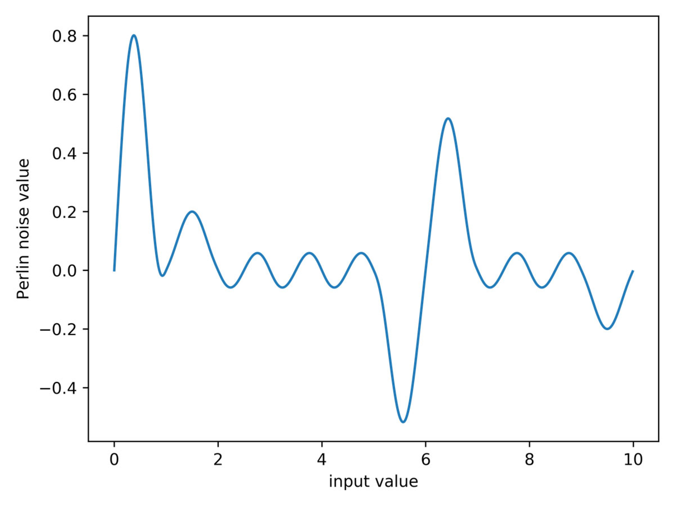
3.1. Stochastic Wind Field Based on Perlin Noise

Only horizontal and vertical wind fields are not sufficient to reflect the full details of the wind field. In nature, the wind field is irregular and usually has a certain degree of randomness. Therefore, we use Perlin noise [43] to simulate the stochastic wind field. Perlin noise is a type of gradient noise, and has a pseudo-random appearance. For the same input value, the same random number will be generated (Figure 1). This is helpful to reflect the random and irregular change of wind fields.

In order to generate different random numbers, we used millisecond time stamp as a random number seed of Perlin noise:

$$\{\begin{array}{l}{v}_{i,x}=\mathit{PerlinNoise}\left(x_i,A,\mathit{tseed}\right)\\ v_{i,y}=\mathit{PerlinNoise}\left(x_i,A,\mathit{tseed}+1\right)\\ v_{i,z}=\mathit{PerlinNoise}\left(x_i,A,\mathit{tseed}-1\right)\end{array},$$

(22)

where $v_{i,x}$, $v_{i,y}$, and $v_{i,z}$ are the components of the velocity $v_{i,\mathit{rand}}$ under the action of the stochastic wind field, and $v_{i,\mathit{rand}}=\left(v_{i,x},v_{i,y},v_{i,z}\right)$. $\mathit{tseed}$ is a millisecond random seed. $x_i$ is the three-dimensional coordinate of the particle $i$. The basic noise generated by Perlin function is between $\left[-1,1\right]$, so we added an amplitude $A$ to adjust the stochastic wind velocity change generated by Perlin function.

We combined the constant wind field $v_{i,\mathit{hori}}$ in the horizontal direction with the stochastic wind field $v_{i,\mathit{rand}}$ produced by Perlin noise to generate a new stochastic wind field. Among them, the constant horizontal wind field plays a leading role. The value of horizontal wind speed is mainly set according to the Beaufort wind scale. The amplitude $A$ of Perlin noise is usually not too large, and the stochastic wind field only plays a certain disturbing action.

$$v_{\mathit{ref}}=v_{i,\mathit{hori}}+v_{i,\mathit{rand}},$$

(23)

where $v_{\mathit{ref}}$ is the reference wind velocity at a reference height $h_{\mathit{ref}}$ from the bottom of the water, and $h_{\mathit{ref}}=10 \mathrm{m}$, which is mainly affected by the Beaufort wind scale, and disturbed by the Perlin stochastic wind field.

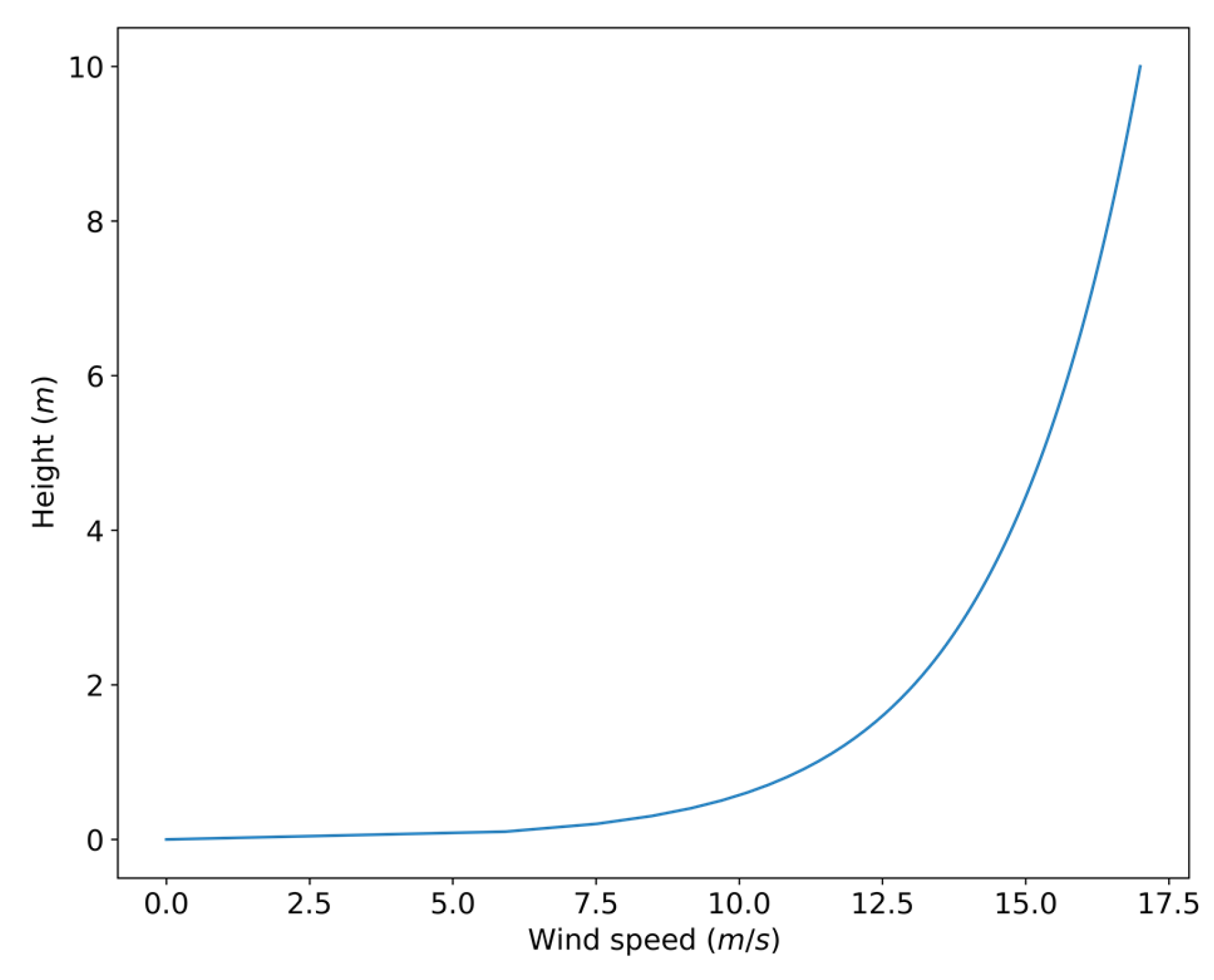
3.2. Wind Profile in the Vertical Direction

When the wind acts on the ocean surface, without considering other external forces, the ocean surface begins to move along the wind direction. Affected by internal friction, seawater in a certain depth range will follow the wind. However, due to factors such as viscosity, the velocity of ocean particles at different depths is different, which is the vertical velocity attenuation. In the wind field, affected by the surface roughness, this attenuation also exists, which is usually described as a wind profile (as shown in Figure 2). Therefore, inspired by the log wind profile equation, we modeled the attenuation of ocean particle velocity of ocean particles with depth.

In this paper, we refer to the form of wind profile equation and adopt a semi-empirical logarithmic form ocean particle velocity attenuation curve:

$$∆v_{i,\mathit{wind}}=\frac{v_{i,\mathit{wind}}^{*}}{\kappa }\ln \left(\frac{z_i+z_0}{z_0}\right),$$

(24)

where $∆v_{i,\mathit{wind}}$ is the velocity change of ocean particle $i$ caused by the wind field, $v_{i,\mathit{wind}}^{*}$ is the friction velocity ($\mathrm{m}/\mathrm{s}$), $\kappa$ is the Von Kármán constant, and $\kappa =0.41$. $z_i$ denotes the vertical coordinate value of ocean particle $i$. $z_0$ is the roughness length of zero plane, and $z_0=0.01$. The friction velocity $v_{i,\mathit{wind}}^{*}$ can be calculated by the following equation:

$$v_{i,\mathit{wind}}^{*}=\frac{\kappa v_{\mathit{ref}}}{\ln \left(\frac{h_{\mathit{ref}}+z_0}{z_0}\right)},$$

(25)

Due to the large difference between the density of air and water, the wind velocity in air cannot be directly applied to fluid particles. Therefore, we introduced a conversion factor based on the density ratio to convert the wind velocity in the air to the fluid particles:

$$∆v_{i,\mathit{wind}}=\beta \frac{{\rho }_{\mathit{air}}}{{\rho }_i}∆v_{i,\mathit{wind}},$$

(26)

where $\beta$ is a control factor, which is used to control the intensity of wind. Generally, the value of $\beta$ should not be too large. ${\rho }_{\mathit{air}}$ is the density of air and ${\rho }_{\mathit{air}}=1.293 \mathrm{kg}/{\mathrm{m}}^3$.

In order to simulate realistic wind waves, we constructed a fluctuating wind field based on the above wind field model. In the fluctuating wind field, the wind periodically acts on the sea surface, as shown in Figure 3. The calculation flow of the wind field model is shown in Appendix C and that of the whole DFPBF model is shown in Appendix D.

4. Results and Discussion

We verified the stability and convergence of our DFPBF method and the Perlin noise-based wind field model by simulating various marine scenes in marine simulators, such as dam break scenes and some coupling scenes. The specific configurations of the computer used in our experiment are AMD Ryzen 7 3700X 8-Core CPU (3.59 GHz), RAM 31.90 GB, and NVIDIA GeForce GTX 2070 SUPER GPU. The physical model was implemented using C++, the rendering part was based on modern OpenGL, and the integrated development environment was Microsoft Visual Studio 2019.

In this section, we call the divergence-free PBF model that does not use the relaxation factor to update position and velocity as DFPBF, and the divergence-free PBF model that uses the relaxation factor to update position and velocity as rDFPBF. Unless otherwise stated, the time steps in the experiments adopt the adaptive scheme in 25 and the particle radius is 0.025L.

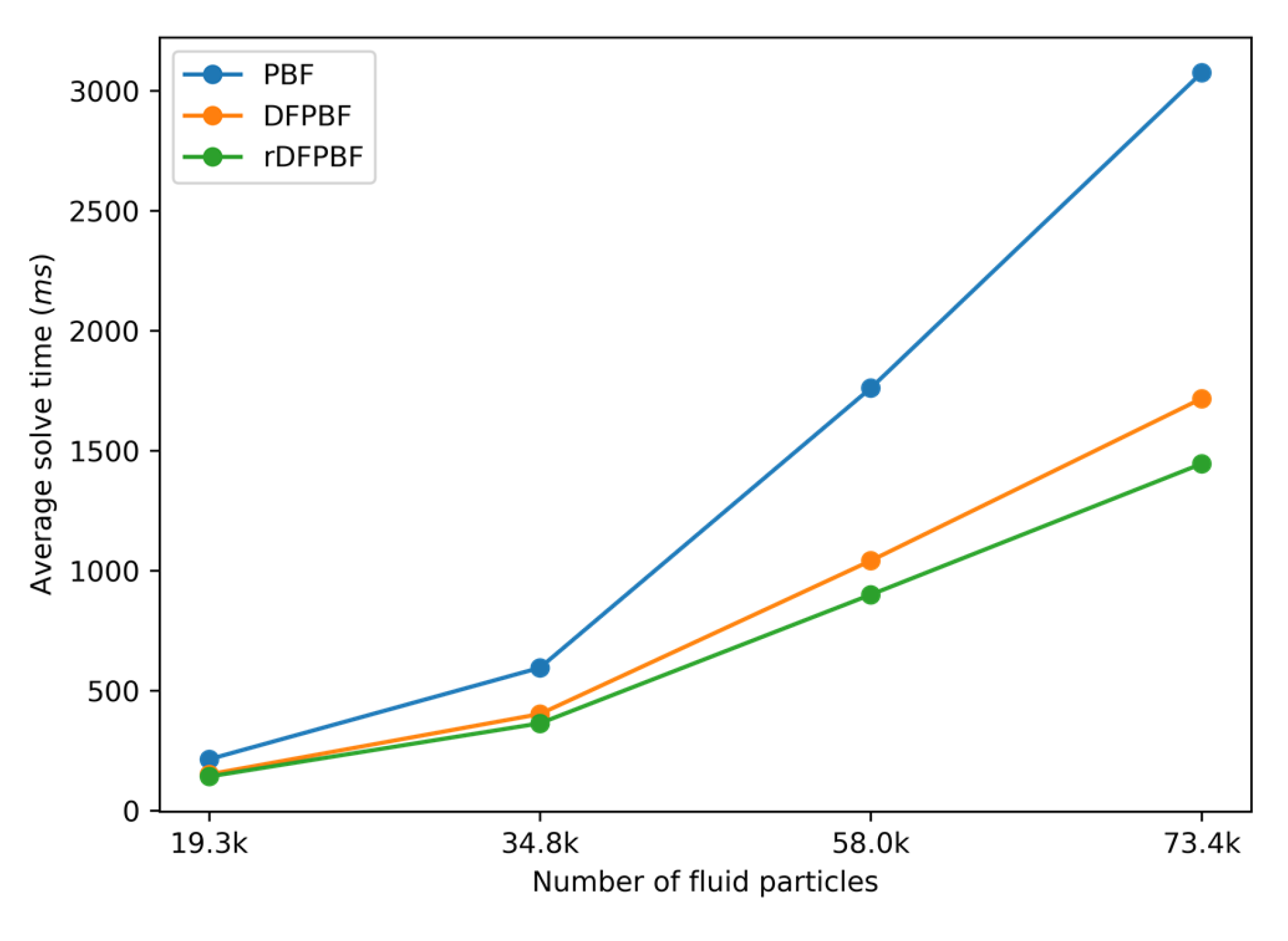
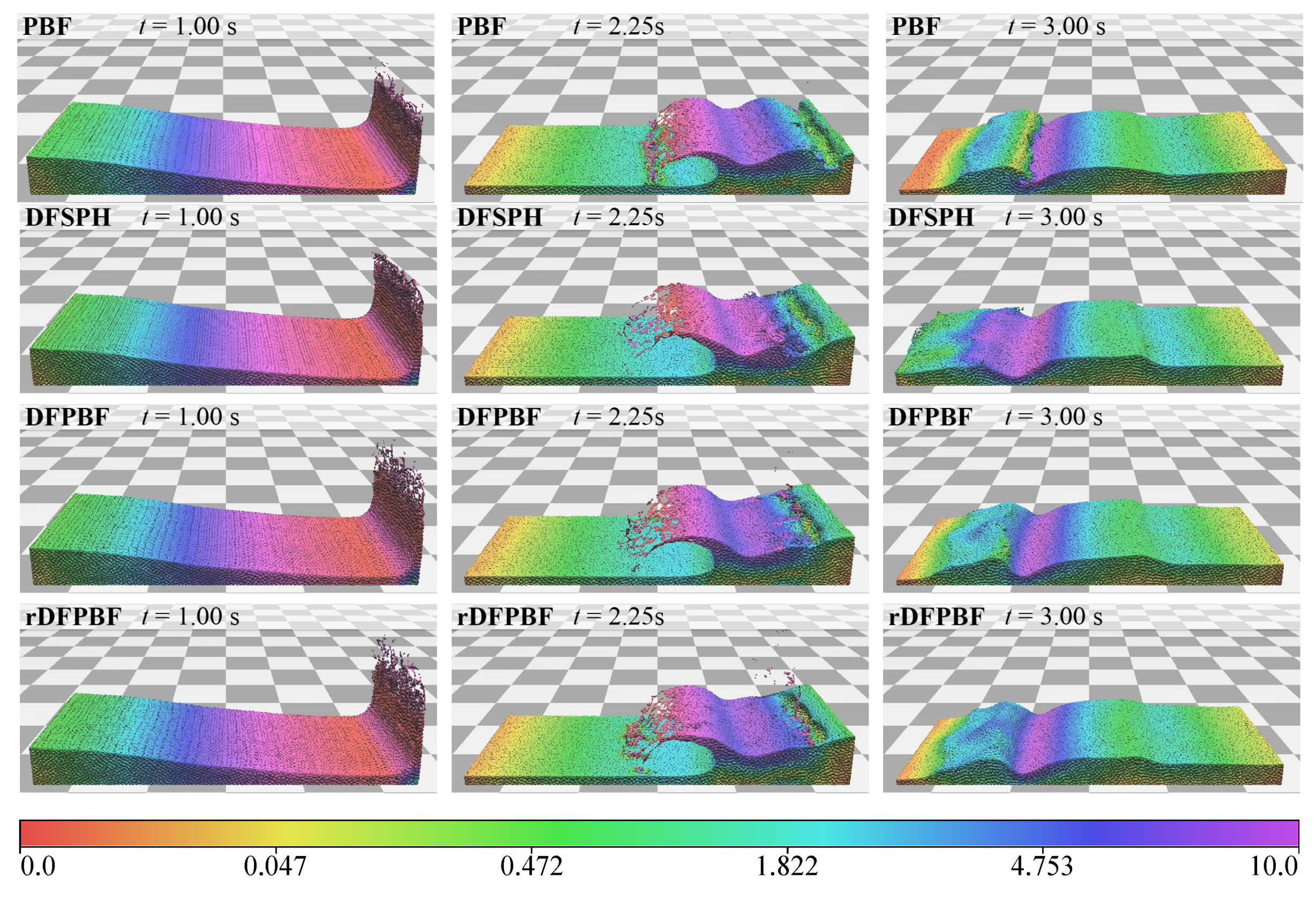
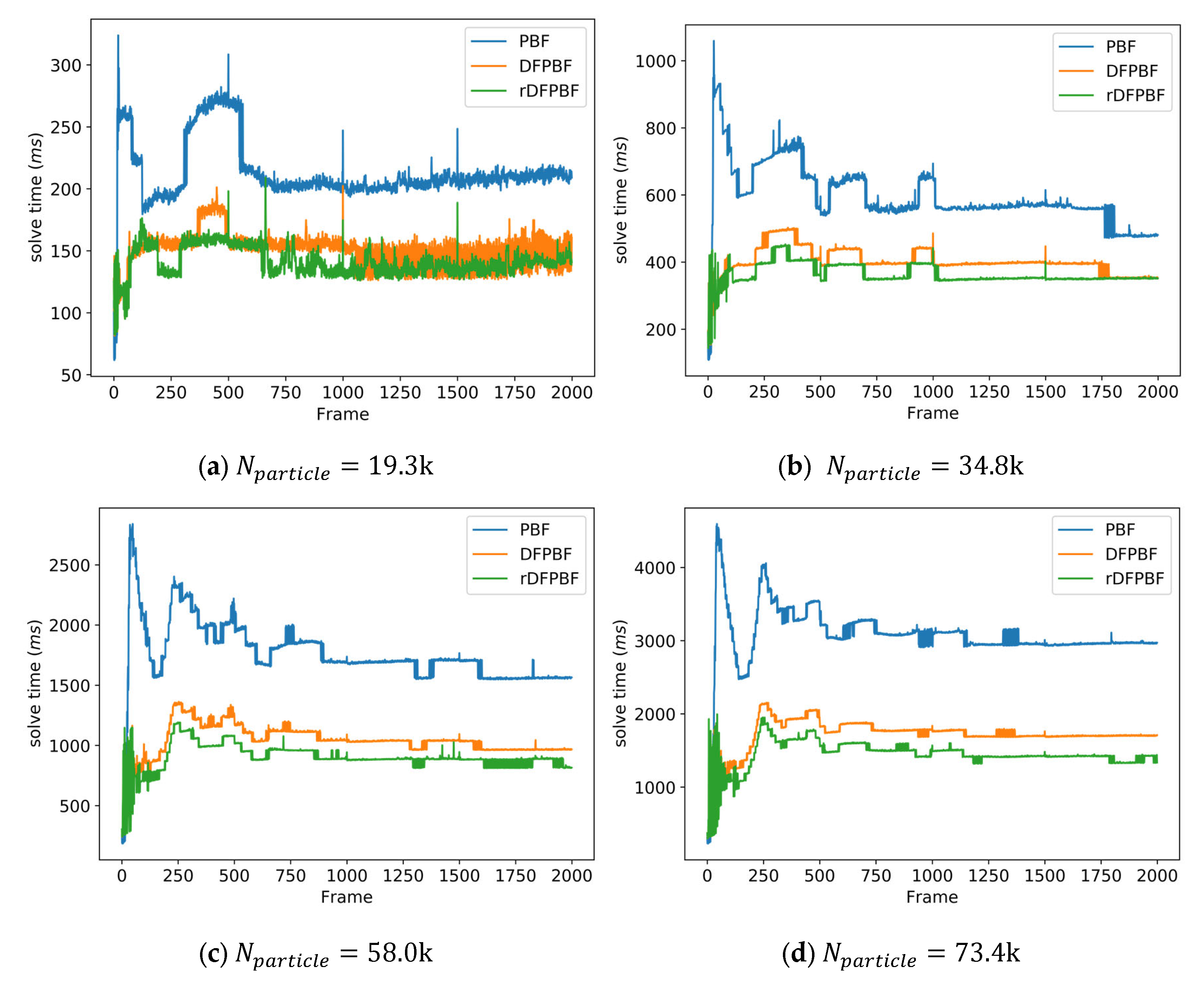
4.1. Performance of DFPBF

We designed a dam break scenario to observe the performance of our DFPBF methods. Figure 4 is the design drawing of the dam break scene. In Figure 4, detailed experimental parameters are given in front and side views. The blue area represents the fluid block and the thick wireframe represents the bounding box. The detailed dimensions of the bounding box in the $x,y$, and $z$ axes are 6L × 3L × 4L. The detailed dimensions of the fluid block at the center of the bottom of the bounding box in the $x, y$, and $z$ directions are 5L × 0.5L × 2L. The fluid block moves only under the influence of gravity.

In order to observe the incompressibility of our DFPBF method, we recorded the maximum density and average density of all fluid particles in each time step, as shown in Figure 5. The closer the density value is to the rest density, the better the incompressibility of the method. In Figure 5, the fluctuation of the average density and the maximum density of the DFPBF method is more obvious, and the incompressibility is relatively poor. While accelerating the convergence, the incompressibility decreases. Moreover, as the relaxation factor increases, the incompressibility of the rDFPBF method will gradually decrease. But for marine simulator, the calculation speed is often the most important factor to be considered, so the rDFPBF method is still attractive. In Figure 5b, the maximum density values of the PBF and DFPBF methods are similar. But in Figure 5a, before the 660th time step, the average density of the PBF method is closer to the rest density than the DFPBF method, but after the 660th time step, the DFBBF method is closer to the rest density.

We tested the convergence of the three methods based on the scenario in Figure 4. The experiments were performed with an average density error of less than 0.01% and 0.001%, respectively, as shown in

Table 1. Comparison of the average iteration number of different methods. Experiments were performed at both compression rates of 0.01% and 0.001%.

Method	Compressibility: 0.01%			Compressibility: 0.001%
	Density Solver	Velocity Solver	Total	Density Solver	Velocity Solver	Total
PBF	9.7	0	9.7	15.8	0	15.8
DFPBF	9.4	1.3	10.7	15.4	1.3	16.7
rDFPBF	6.9	1.5	8.5	10.6	1.5	12.1

. In all the experiments, the density change rate error in the velocity solver is less than 0.1%. The number of fluid particles in the scene is 34.8k. In terms of boundary conditions, a non-uniform single-layer boundary particle model is used, and the number of boundary particles after sampling is 106.2k. The mass of the boundary particles is the same as that of the fluid particles, but the velocity of the boundary particles in all directions is 0.

As shown in Appendix D, in our DFPBF framework, the parameter ${\alpha }_i$ is computed once in each time step and will not be updated in the iteration. We have experimented with many scenarios, this scheme is relatively stable, and speeds up the calculation. But in some multiphase flow scenarios, ${\alpha }_i$ needs to be updated in each iteration, but it is beyond the scope of this paper. In Table 1, the convergence of the rDFPBF method is the best, especially in the constant density solver, compared with the other two methods, we can see a significant improvement in convergence. In the constant density solver, the convergence of the DFPBF method is slightly better than that of the PBF method, but because of the divergent-free solver, the total number of iterations is increased. From the number of iterations of the divergence-free solver in Table 1, it can be seen that when updating the velocity, the use of a relaxation factor leads to an increase in the number of iterations. Therefore, in practical applications, we recommend adjusting the relaxation scheme according to the actual situation, that is, the relaxation scheme can only be used in the solver with slow convergence. If the convergence speed is fast, the relaxation factor can be omitted.

As the iteration scheme of the methods changes, the calculation time will also change. With an average density error of less than 0.01% in the constant density solver, we analyzed the time consumption of the methods, as shown in

Table 2. Average time consumption of density constraint solvers in PBF and RPBF methods.

Particle Number	Block Size	PBF (ms)	RPBF (ms)	rDFPBF (ms)
19.3k	5L × 0.3L × 2L	213.24	150.41	141.39
34.8k	5L × 0.5L × 2L	594.73	401.90	363.10
58.0k	5L × 0.8L × 2L	1760.28	1040.89	899.35
73.4k	5L × 1.0L × 2L	3074.52	1716.63	1444.79

. In this group of experiments, the time step is 0.005 s. The result of time consumption is usually different with different number of fluid particles. Therefore, by setting different fluid block sizes (Figure 6 and Table 2), we have listed the analysis results of four different numbers of fluid particles (19.3k, 34.8k, 58.0k, 73.4k). It can be seen from Figure 6 that the DFPBF method and the rDFPBF method using the improved iterative scheme have a faster calculation speed. Figure 7 is the visualization result of Table 2. In Figure 7, as the number of fluid particles increases, the calculation speed increases more significantly. This is attractive for the simulation of real-time fluid scene in virtual reality.

We visualized the dam break scenario based on the PBF, DFSPH, DFPBF, and rDFPBF methods, respectively. As shown in Figure 8, the size of the fluid block in the scene is 1.5L × 1.5L × 2L, and the size of the bounding box is 5L × 5L × 2L. The particle radius is 0.02L and the number of fluid particles is 67.1k. The time step size is 0.005 s. In Figure 8, the color of the fluid particles represents the particle velocity. Since there are only a few fluid particles with larger velocity, in order to observe most low velocity particles, the color bar in Figure 8 adopts a nonlinear mapping. We selected three different time instants (1.00 s, 2.25 s, and 3.00 s) from the dam-break scenarios simulated by each method. As can be seen from Figure 8, compared with PBF method and the DFSPH method, the fluids simulated by our DFPBF method and the rDFPBF method have a similar velocity distribution.

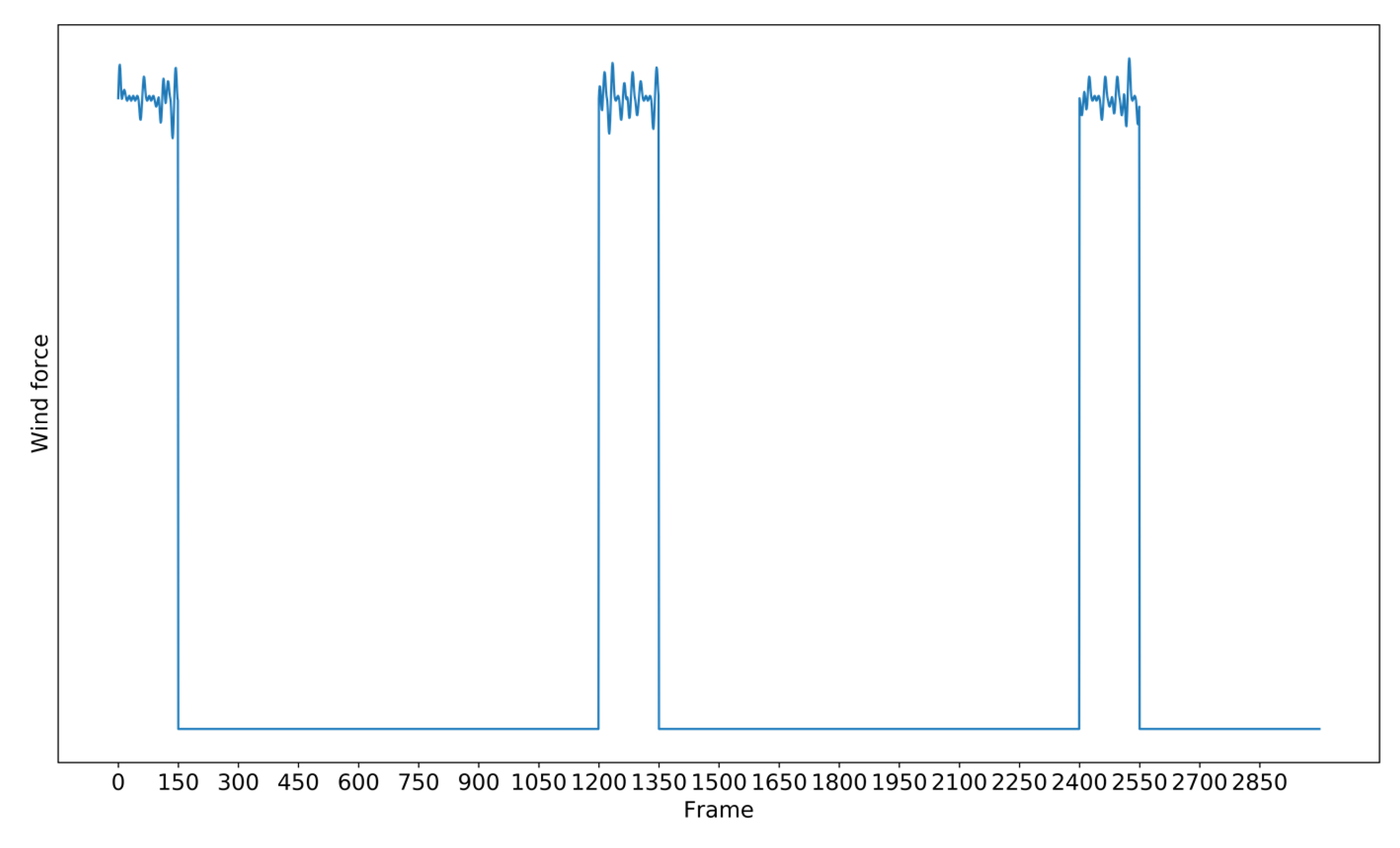
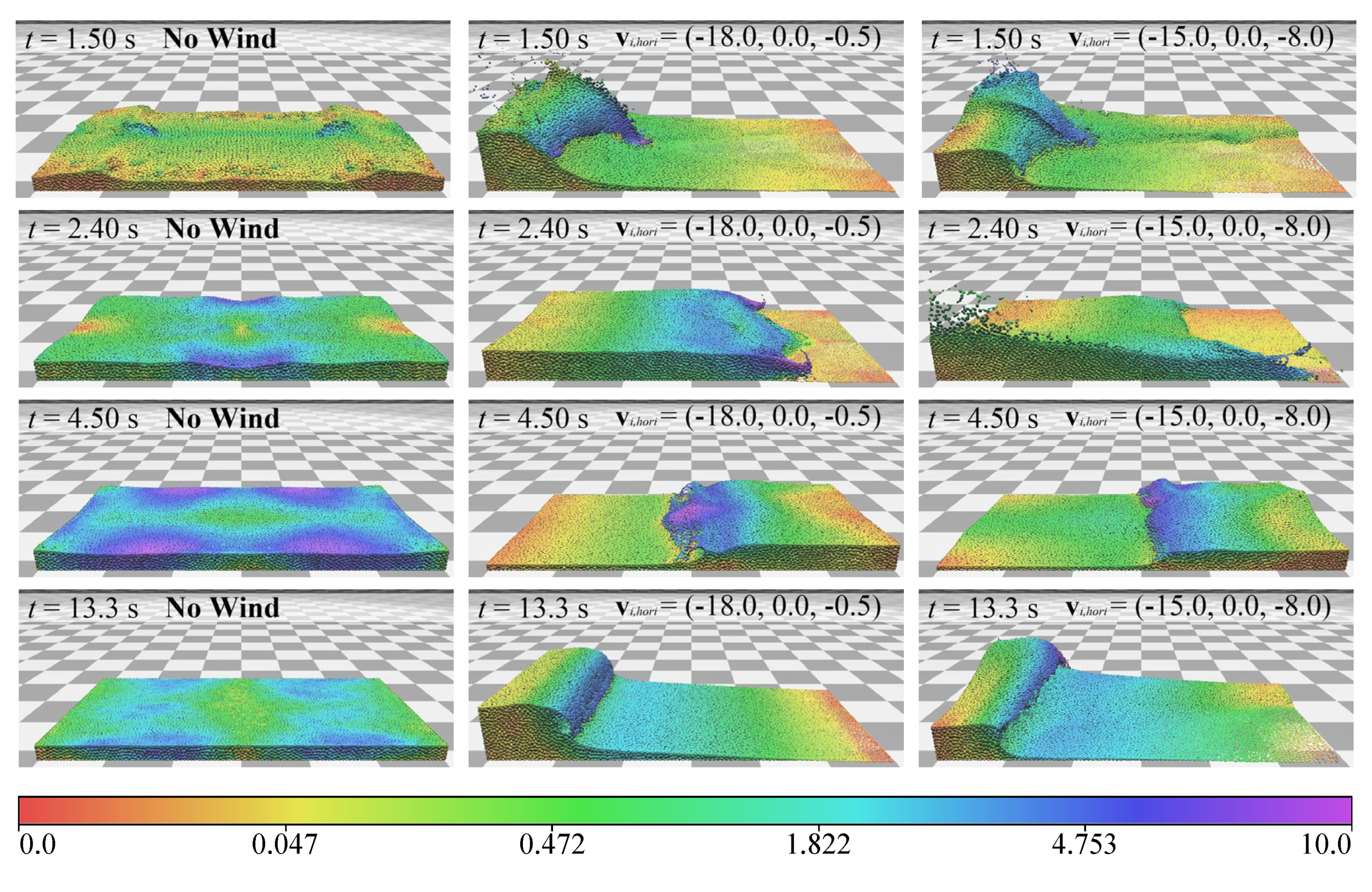
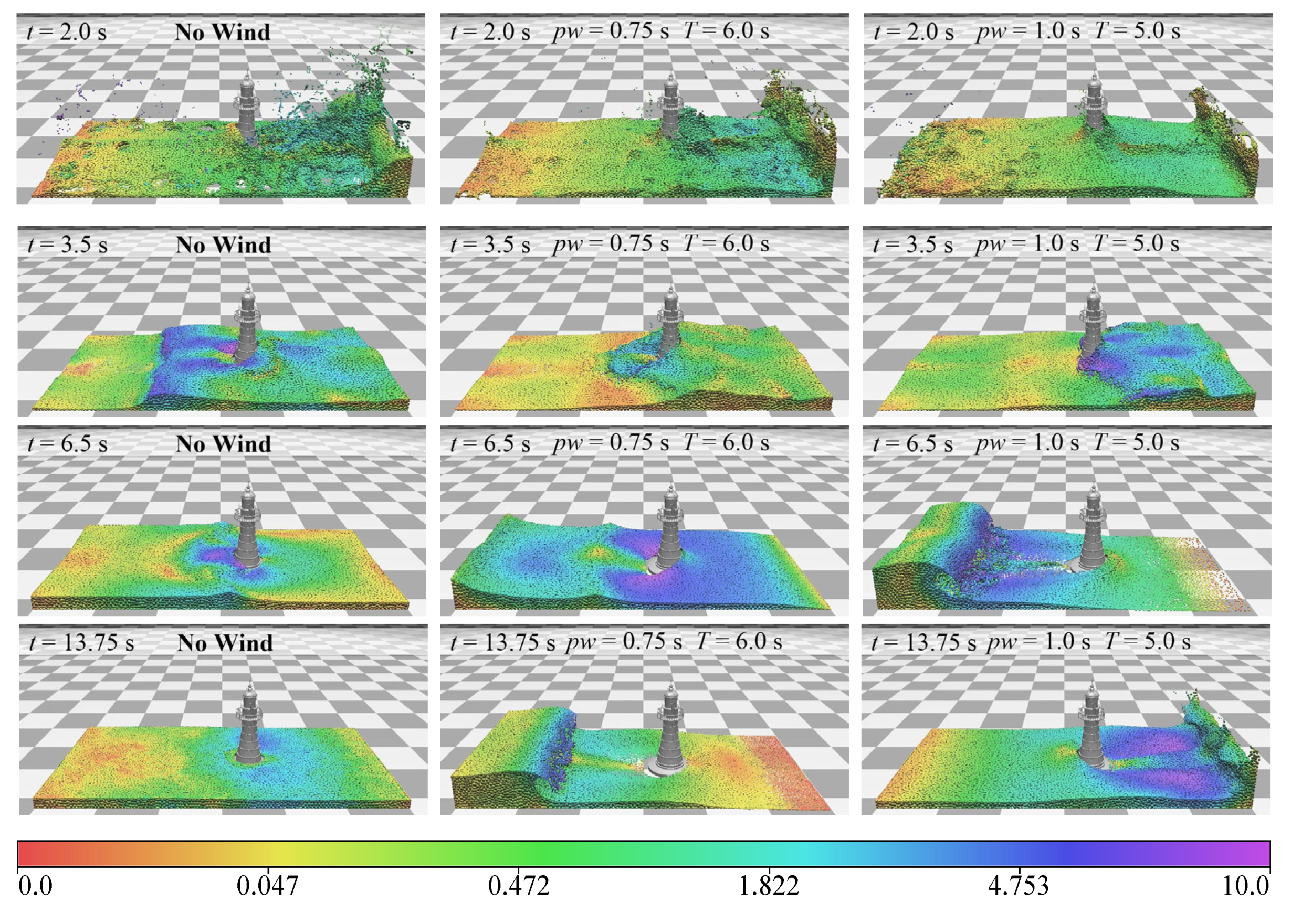
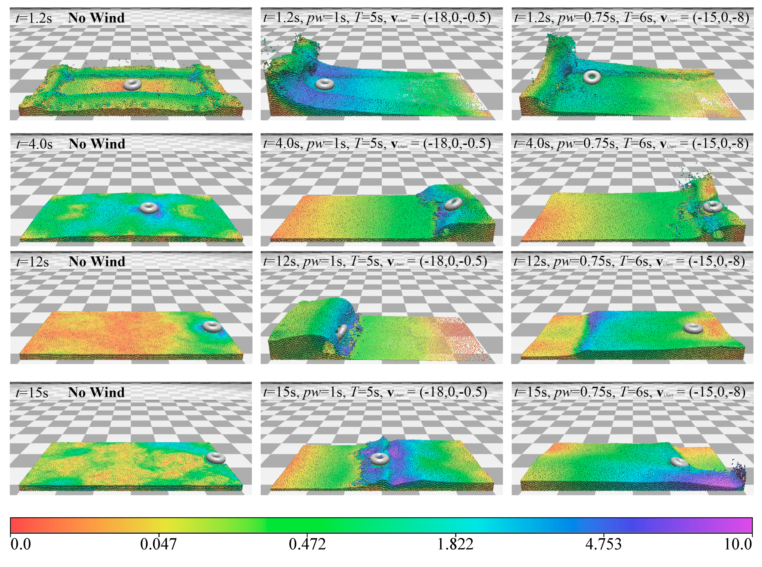
4.2. Wind Field Simulation Results

We simulated some typical wind wave scenarios in marine simulators based on our stochastic fluctuating wind field model. In the scenario shown in Figure 9, the size of the fluid block is 5L × L × 2L and that of the bounding box is 6L × 5L × 3L. The number of fluid particles is 57.9k. The time step is 0.005 s. As described in Section 3.2, we use a stochastic fluctuating wind field with a pulse period of 6 s and a pulse width of the first 0.75 s within each pulse period in Figure 9. The amplitude $A$ in Equation (22) is set to 3.0, and the control factor $\beta =1.5$. Figure 9 shows the results of the wind field with different initial wind velocities. We select some typical time instants (1.50 s, 2.40 s, 4.50 s, and 13.3 s) to observe the sea surface under the action of different wind fields. According to the log wind profile, due to the different height of fluid particles, the wind forces exerted on the fluid particles are also different. The velocity of the particles at high altitudes is relatively large. Adding the reaction force of the dam, it is easy to generate wave overturning, as shown in the time instant of 13.3 s in Figure 9.

In order to verify the applicability of the proposed wind field model in interactive scenarios, we designed two interactive scenarios experiments. In all the fluid-rigid coupling scenes, the Poisson disk sampling method [44] was used to sample all rigid bodies including bounding boxes as rigid particles. We adopted single layer non-uniform boundary particle model [45] to deal with the two-way coupling situations. In all static rigid bodies, such as lighthouse and bounding boxes, the velocity of rigid particles is 0.

The static object interaction scene is shown in Figure 10. The specific parameters about the scene have been marked in the design diagram. The number of fluid particles is 44.1 k. The time step is 0.005 s. At the same initial wind velocity $v_{i,\mathit{hori}}=\left(-18,0,-0.5\right)$, we simulated the sea surface under the action of wind fields with different pulse periods and different pulse widths. In Figure 11, in the left column of the images, the fluid particles move only under the influence of gravity, and when no wind field is applied. In the images in the middle column of Figure 11, the fluid particles move under the action of gravity and wind field. The pulse period $T$ lasts for 6 s, and the pulse width $\mathit{pw}$ is the first 0.75 s in each period. In the images on the right column, the pulse period $T$ lasts for 5 s, and the pulse width $\mathit{pw}$ is the first second in each period. The amplitude $A$ in Equation (22) is set to 3.0, and the control factor $\beta =1.5$. As shown in Figure 11, in the instants at 2.0 s and 3.50 s, the wind field acts in the opposite direction to the dam break, so it cancels out some of the kinetic energy. Therefore, the greater the wind, the less the kinetic energy. However, in the instants shown in 6.5 s and 13.75 s, the water surface without wind gradually became calmer, while the water surface under the action of wind fluctuates violently.

A lifebuoy is selected as a dynamic object to dynamically interact with ocean waves. The specific parameters of the scene are indicated in the design drawing (Figure 12). The number of particles is $46.8\mathrm{k}$. The time step is 0.005 s. In Figure 13, we compared the movement of the lifebuoy falling into water under different wind conditions. The images in the left column of Figure 13 show the falling motion of the lifebuoy under windless conditions. The initial wind velocity $v_{i,\mathit{hori}}$ in the images in the middle column of Figure 13 is $\left(-18,0,-0.5\right)$, the pulse period $T$ lasts for 5 s, and the pulse width $\mathit{pw}$ is the first second in each pulse period. The initial wind velocity $v_{i,\mathit{hori}}$ in the images in the right column of Figure 13 is $\left(-15,0,-8\right)$, the pulse period lasts $T$ for 6 s, and the pulse width $\mathit{pw}$ is the first 0.75 s in each pulse period. The control factor $\beta$ is 1.5. Since the lifebuoy is a dynamic boundary, it is different from the static boundary in boundary treatment. The lifebuoy is also sampled as boundary particles with the same mass as fluid particles, but the velocity of boundary particles is computed according to the rigid body motion model.

5. Conclusions and Future Work

In order to simplify the modeling of splash scenes in marine simulators and enhance physical reality, we introduce an improved DFPBF model to model ocean waves. We added a set of improved divergent-free velocity constraints to the original PBF framework to minimize the density change rate, and improved the iterative process of the density constraint solver. After experimental verification, our DFPBF method not only has a similar incompressibility to PBF but also significantly accelerates the calculation speed, and with the increase of fluid particles, this acceleration advantage will be more obvious, which is very suitable for real-time fluid simulation. On the basis of DFPBF, we introduced a relaxation scheme when updating the velocity and position according to the constraints. Although the incompressibility is weakened, the calculation speed has been improved and can be used as an attractive backup in practical applications. If the applications pay more attention to rapidity, then the rDFPBF method is a better solution. In addition, we propose an empirical model of stochastic fluctuating wind field, which can be easily integrated into the DFPBF framework. In this wind field model, we reserve some parameters for users to flexibly control wind special effects. The wind field model greatly enriches the details of wind and waves in marine simulator.

There are still some possibilities to improve our method. In terms of the relaxation factor, different incompressibility may apply to different relaxation factors. Moreover, in the relaxation scheme, the constant density solver and the divergence-free solver may not apply the relaxation scheme at the same time. The generation of Perlin noise takes some time, which affects the simulation speed of the scene. But if Perlin noise can be accelerated in parallel, then its efficiency will be greatly improved.

References

1. Tessendorf, J. Simulating Ocean Water; 2004 Course Notes; ACM SIGGRAPH: Los Angeles, CA, USA, 2004. [Google Scholar]
2. Pierson, W.J., Jr.; Moskowitz, L. A proposed spectral form for fully developed wind seas based on the similarity theory of SA Kitaigorodskii. J. Geophys. Res. 1964, 69, 5181–5190. [Google Scholar] [CrossRef]
3. Horvath, C.J. Empirical directional wave spectra for computer graphics. In Proceedings of the 2015 Symposium on Digital Production, Los Angeles, CA, USA, 8 August 2015; Association for Computing Machinery: New York, NY, USA, 2015; pp. 29–39. [Google Scholar]
4. Hasselmann, K.; Barnett, T.P.; Bouws, E.; Carlson, H.; Cartwright, D.E.; Enke, K.; Ewing, J.A.; Gienapp, H.; Hasselmann, D.E.; Kruseman, P.; et al. Measurements of wind-wave growth and swell decay during the Joint North Sea Wave Project (JONSWAP). Ergänzung Deut. Hydrogr. Z. 1973, 12, 1–95. [Google Scholar]
5. Fréchot, J. Realistic simulation of ocean surface using wave spectra. In Proceedings of the First International Conference on Computer Graphics Theory and Applications, Setúbal, Portugal, 25–28 February 2006; Springer: Berlin/Heidelberg, Germany, 2007; pp. 76–83. [Google Scholar]
6. Bouws, E.; Günther, H.; Rosenthal, W.; Vincent, C.L. Similarity of the wind wave spectrum in finite depth water: 1. Spectral form. J. Geophys. Res. Oceans 1985, 90, 975–986. [Google Scholar] [CrossRef]
7. Lee, N.; Baek, N.; Ryu, K.W. A real-time method for ocean surface simulation using the TMA model. Int. J. Comput. Inf. Syst. Ind. Manag. Appl. 2009, 1, 25–26. [Google Scholar]
8. Kitaigordskii, S.A.; Krasitskii, V.P.; Zaslavskii, M.M. On Phillips’ theory of equilibrium range in the spectra of wind-generated gravity waves. J. Phys. Oceanogr. 1975, 5, 410–420. [Google Scholar] [CrossRef] [Green Version]
9. Hughes, S.A. The TMA Shallow-Water Spectrum Description and Applications; Tech. Rep. CERC-84-7; Coastal Engineering Research Center: Vicksburg, MS, USA, 1984. [Google Scholar]
10. Chen, L.; Jin, Y.; Yin, Y. Ocean wave rendering with whitecap in the visual system of a maritime simulator. J. Comput. Inf. Technol. 2017, 25, 63–76. [Google Scholar] [CrossRef] [Green Version]
11. Irving, G.; Guendelman, E.; Losasso, F.; Fedkiw, R. Efficient simulation of large bodies of water by coupling two and three dimensional techniques. ACM Trans. Graph. 2006, 25, 805–811. [Google Scholar] [CrossRef]
12. Chentanez, N.; Müller, M. Real-time Eulerian water simulation using a restricted tall cell grid. ACM Trans. Graph. 2011, 30, 82. [Google Scholar] [CrossRef]
13. Lucy, L.B. A numerical approach to the testing of the fission hypothesis. Astron. J. 1977, 82, 1013–1024. [Google Scholar] [CrossRef]
14. Gingold, R.A.; Monaghan, J.J. Smoothed particle hydrodynamics: Theory and application to non-spherical stars. Mon. Not. R. Astron. Soc. 1977, 181, 375–389. [Google Scholar] [CrossRef]
15. Liu, G.R.; Liu, M.B. Smoothed Particle Hydrodynamics: A Meshfree Particle Method; World Scientific Publishing Company: Singapore, 2003. [Google Scholar]
16. Stam, J.; Fiume, E. Depicting fire and other gaseous phenomena using diffusion processes. In Proceedings of the 22nd Annual Conference on Computer Graphics and Interactive Techniques, Los Angeles, CA, USA, 6–11 August 1995; Mair, S.G., Cook, R., Eds.; Association for Computing Machinery: New York, NY, USA, 2003; pp. 129–136. [Google Scholar]
17. Müller, M.; Charypar, D.; Gross, M. Particle-based fluid simulation for interactive applications. In Proceedings of the 2003 ACM SIGGRAPH/Eurographics symposium on Computer animation, San Diego, CA, USA, 26–27 July 2003; Eurographics Association: Goslar, Germany, 2003; pp. 154–159. [Google Scholar]
18. Monaghan, J.J. Simulating free surface flows with SPH. J. Comput. Phys. 1994, 110, 399–406. [Google Scholar] [CrossRef]
19. Becker, M.; Teschner, M. Weakly compressible SPH for free surface flows. In Proceedings of the 2007 ACM SIGGRAPH/Eurographics Symposium on Computer Animation, San Diego, CA, USA, 2–4 August 2007; Eurographics Association: Goslar, Germany, 2007; pp. 209–218. [Google Scholar]
20. Solenthaler, B.; Pajarola, R. Predictive-corrective incompressible SPH. ACM Trans. Graph. 2009, 28, 40. [Google Scholar] [CrossRef] [Green Version]
21. He, X.; Liu, N.; Li, S.; Wang, H.; Wang, G. Local poisson SPH for viscous incompressible fluids. Comput. Graph. Forum 2012, 31, 1948–1958. [Google Scholar] [CrossRef]
22. Shao, S.; Lo, E.Y.M. Incompressible SPH method for simulating Newtonian and non-Newtonian flows with a free surface. Adv. Water Resour. 2003, 26, 787–800. [Google Scholar] [CrossRef]
23. Asai, M.; Aly, A.M.; Sonoda, Y.; Sakai, Y. A stabilized incompressible SPH method by relaxing the density invariance condition. J. Appl. Math. 2012, 2012, 139583. [Google Scholar] [CrossRef]
24. Ihmsen, M.; Cornelis, J.; Solenthaler, B.; Horvath, C.; Teschner, M. Implicit incompressible SPH. IEEE Trans. Vis. Comput. Graph. 2013, 20, 426–435. [Google Scholar] [CrossRef]
25. Bender, J.; Koschier, D. Divergence-free smoothed particle hydrodynamics. In Proceedings of the 14th ACM SIGGRAPH/Eurographics Symposium on Computer Animation, Los Angeles, CA, USA, 7–9 August 2015; Eurographics Association: Goslar, Germany, 2015; pp. 147–155. [Google Scholar]
26. Cornelis, J.; Bender, J.; Gissler, C.; Ihmsen, M.; Teschner, M. An optimized source term formulation for incompressible SPH. Visual Comput. 2019, 35, 579–590. [Google Scholar] [CrossRef]
27. Müller, M.; Heidelberger, B.; Hennix, M.; Ratcliff, J. Position based dynamics. J. Vis. Commun. Image Represent. 2007, 18, 109–118. [Google Scholar] [CrossRef] [Green Version]
28. Macklin, M.; Müller, M. Position based fluids. ACM Trans. Graph. 2013, 32, 104. [Google Scholar] [CrossRef]
29. Bodin, K.; Lacoursière, C.; Servin, M. Constraint fluids. IEEE Trans. Vis. Comput. Graph. 2012, 18, 516–526. [Google Scholar] [CrossRef]
30. Kang, N.; Sagong, D. Incompressible SPH using the divergence-free condition. Comput. Graph. Forum. 2014, 33, 219–228. [Google Scholar] [CrossRef]
31. Müller, M.; Solenthaler, B.; Keiser, R.; Gross, M. Particle-based fluid-fluid interaction. In Proceedings of the 2005 ACM SIGGRAPH/Eurographics Symposium on Computer Animation, Los Angeles, CA, USA, 29–31 July 2005; Association for Computing Machinery: New York, NY, USA, 2005; pp. 237–244. [Google Scholar]
32. Ihmsen, M.; Bader, J.; Akinci, G.; Teschner, M. Animation of air bubbles with SPH. In Proceedings of the International Conference on Computer Graphics Theory and Applications, Vilamoura, Algarve, Portugal, 5–7 March 2011; Institute for Systems and Technologies of Information, Control and Communication: Setubal, Portugal, 2011; pp. 225–234. [Google Scholar]
33. Ihmsen, M.; Akinci, N.; Akinci, G.; Teschner, M. Unified spray, foam and air bubbles for particle-based fluids. Visual Comput. 2012, 28, 669–677. [Google Scholar] [CrossRef]
34. Macklin, M.; Müller, M.; Chentanez, N.; Kim, T.Y. Unified particle physics for real-time applications. ACM Trans. Graph. 2014, 33, 1–12. [Google Scholar] [CrossRef]
35. Gissler, C.; Band, S.; Peer, A.; Ihmsen, M.; Teschner, M. Approximate air-fluid interactions for SPH. In Proceedings of the 13th Workshop on Virtual Reality Interaction and Physical Simulation, Lyon, France, 23–24 April 2017; Eurographics Association: Goslar, Germany, 2017; pp. 29–38. [Google Scholar]
36. Akinci, N.; Ihmsen, M.; Akinci, G.; Solenthaler, B.; Teschner, M. Versatile rigid-fluid coupling for incompressible SPH. ACM Trans. Graph. 2012, 31, 62. [Google Scholar] [CrossRef]
37. Bender, J.; Koschier, D.; Kugelstadt, T.; Weiler, M. A micropolar material model for turbulent SPH fluids. In Proceedings of the ACM SIGGRAPH/Eurographics Symposium on Computer Animation, Los Angeles, CA, USA, 28–30 July 2017; Association for Computing Machinery: New York, NY, USA, 2017; p. 4. [Google Scholar]
38. Bender, J.; Koschier, D.; Kugelstadt, T.; Weiler, M. Turbulent Micropolar SPH fluids with foam. IEEE Trans. Vis. Comput. Graph. 2018, 25, 2284–2295. [Google Scholar] [CrossRef]
39. Losasso, F.; Talton, J.O.; Kwatra, N.; Fedkiw, R. Two-way coupled SPH and particle level set fluid simulation. IEEE Trans. Vis. Comput. Graph. 2008, 14, 797–804. [Google Scholar] [CrossRef] [PubMed]
40. Monaghan, J.J.; Gingold, R.A. Shock simulation by the particle method SPH. J. Comput. Phys. 1983, 52, 374–389. [Google Scholar] [CrossRef]
41. Monaghan, J.J. Smoothed particle hydrodynamics. Annu. Rev. Astron. Astrophys. 1992, 30, 543–574. [Google Scholar] [CrossRef]
42. Ihmsen, M.; Orthmann, J.; Solenthaler, B.; Kolb, A.; Teschner, M. SPH Fluids in Computer Graphics; EG2014–STARs: Strasbourg, France, 2014. [Google Scholar]
43. Perlin, K. Improving Noise. ACM Trans. Graph. 2002, 21, 681–682. [Google Scholar] [CrossRef]
44. Bowers, J.; Wang, R.; Wei, L.Y.; Maletz, D. Parallel Poisson disk sampling with spectrum analysis on surfaces. ACM Trans. Graph. 2010, 29, 166. [Google Scholar] [CrossRef]
45. Li, H.; Ren, H.; Qiu, S.; Wang, C. Physics-Based Simulation of Ocean Scenes in Marine Simulator Visual System. Water 2020, 12, 215. [Google Scholar] [CrossRef] [Green Version]
Figure 1. An example of one-dimensional Perlin noise. The abscissa represents the input value between [0,10], the interval is 0.01, and the ordinate is the noise value.
Water 12 01873 g001
Figure 2. Schematic diagram of one-dimensional log wind profile. The reference wind speed is 17 m/s and the reference height is 10 m. The control factor β is 1.0.
Water 12 01873 g002
Figure 3. Schematic diagram of fluctuating wind field. Each pulse period lasts 1200 time steps (frames). A stochastic wind field is applied during the first 150 time steps in each pulse period.
Water 12 01873 g003
Figure 4. Design drawing of dam break scene. Image (a) is the front view of the dam break scene, and image (b) are the side view. The front view and side view show the detailed parameters of the bounding box and fluid block. The unit of length used in dam break scene is dimensionless, and its specific length can be set by L .
Water 12 01873 g004
Figure 5. Incompressibility comparison. In images (a) and (b), the black dotted line represents the ideal rest density. The blue curve represents the density of the PBF method, the orange curve represents that of our DFPBF method, and the green curve represents that of the rDFPBF method.
Water 12 01873 g005
Figure 6. Time consumption of the PBF, DFPBF, and rDFPBF methods. The blue curve represents the time consumption of each time step of PBF method. The orange curve shows the time consumption of each time step of DFPBF method. The green curve shows the time consumption of each time step of rDFPBF method. Images (a)–(d) are the results of different number of particles.
Water 12 01873 g006
Figure 7. Average time consumption of the PBF, DFPBF and rDFPBF methods. The blue curve represents the average time consumption of PBF method. The orange curve shows that of DFPBF method. The green curve shows that of rDFPBF method.
Water 12 01873 g007
Figure 8. Scene of dam break with 67.1k fluid particles. The different color in the images are the velocity distributions of fluid particles, which are selected from three different time steps.
Water 12 01873 g008
Figure 9. Fluid block under the action of wind field. The different color in the images are the velocity distributions of fluid particles, and the unit of velocity is m/s.
Water 12 01873 g009
Figure 10. Design drawing of interaction scene between wave and lighthouse affected by wind field. The front and side view show the detailed parameters of the bounding box, lighthouse, and fluid block. In the side view, the lighthouse is located behind the fluid block, thus the lighthouse is represented by dashed lines.
Water 12 01873 g010
Figure 11. Simulation results of interaction scene between wave and lighthouse affected by wind field. The different color in the images are the velocity distributions of fluid particles, and the unit of velocity is m/s.
Water 12 01873 g011
Figure 12. Design drawing of interaction scene between wave and lifebuoy affected by wind field. The front and side view show the detailed parameters of the bounding box, lifebuoy, and fluid block.
Water 12 01873 g012
Figure 13. Simulation results of interaction scene between wave and lifebuoy affected by wind field. The different color in the images are the velocity distributions of fluid particles, and the unit of velocity is m/s.
Water 12 01873 g013