Article

Macro-Turbulent Flow and Its Impacts on Sediment Transport Potential of a Subarctic River during Ice-Covered and Open-Channel Conditions

1
Department of Geographical and Historical Studies, University of Eastern Finland, Yliopistokatu 2, P.O. Box 111, FI-80101 Joensuu, Finland
2
Department of Geography and Geology, University of Turku, Turun yliopisto, FI-20014 Turku, Finland
3
Section 4.6 Geomorphology, German Research Centre for Geosciences GFZ Potsdam, D-14473 Potsdam, Germany
4
Finnish Environment Institute, Latokartanonkaari 11, FI-00790 Helsinki, Finland
5
Finnish Geospatial Research Institute, National Land Survey of Finland, Geodeetinrinne 2, FI-02430 Masala, Finland
6
Turku University of Applied Sciences, Joukahaisenkatu 3, FI-20520 Turku, Finland
*
Author to whom correspondence should be addressed.
Water 2020, 12(7), 1874; https://doi.org/10.3390/w12071874
Submission received: 28 May 2020 / Revised: 22 June 2020 / Accepted: 25 June 2020 / Published: 30 June 2020

Abstract

:
Macro-turbulent flows (i.e., coherent flow structures reaching through the whole water column), have not been studied widely in northern seasonally frozen rivers during both open-channel and ice-covered flow conditions. Thus, we aim: (1) to detect and compare the macro-turbulent flow, both at open-channel and ice-covered flow conditions; (2) to explore spatial variation of macro-turbulent flow characteristics within a meander bend; and (3) to detect the effects of near-bed layer velocity fluctuation on bedload transport during differing overall flow conditions. The analyses are based on 5–10 min-long acoustic Doppler current profiler (ADCP) measurements from a subarctic river. The ice-covered low flow, and open-channel higher and lower flow conditions were measured over the period of 2016 to 2020. This study found that macro-turbulent flow existed at all measurement locations under both open-channel and ice-covered flow conditions. Macro-turbulent flow was most consistent and obvious in the streamwise velocity component, and in particular at the inlet and outlet of the investigated meander bend. During all seasons, the near-bed velocities consistently exceeded the sufficient amount for sediment transport. At inlet and outlet areas, the greatest near-bed velocity fluctuation across the critical threshold for sediment transport coincided with the measurement times having frequent macro-turbulent flow.

1. Introduction

River ice can have a significant impact on the distribution and magnitude of flows in the river channels [1,2,3]. Under ice-covered conditions, increases are seen in the spatial variability and characteristics of depositional and erosional locations compared to the open-channel conditions [3]. However, these observations are based on studies conducted during only one season and on measurements that are too short (less than 1 min) to capture larger pulsating structures of high and low flows. The impact of this flow pulsation on the sediment transport potential and morphology of rivers during open-channel conditions has been studied over several decades (e.g., [4]), and it has been identified that this characteristic likely plays a major role in bedload sediment transport [5,6]. This has been shown in open-channel conditions of natural gravel-bed rivers [5] as well as in open-channel flume experiments [6]. The streamwise velocity component of these high-speed pulses are expected to play a dominant role on sediment transport dynamics [7,8], despite occurring for just a few seconds at any fixed location [5]. Further studies need to verify the impacts of these pulsating flows during both open-channel and ice-covered conditions on the sediment transport, as this study is only aware of Demers et al. [9] who have studied similar conditions at a natural state sand-bed meandering river.
Previous research has termed pulsating flows as macro-turbulent flow structures [10], intermittent high-speed wedges separated by regions of lower velocity [5], boundary-related coherent flow structure (CFS) [7], or macro-turbulent coherent structures (MCS) [9]. According to Sukhodolov et al. [11], turbulence generation in fully developed channel flow is associated with the existence of coherent structures, which are connected with bursting eddies occurring randomly near the bed and behaving in an organized manner. The turbulent bursts have been initially confirmed to occur at the boundary layers of flow [12]. Sukhodolov et al. [11] further described that in two-dimensional flow the bursting phases are represented by a sudden outward motion of low-speed fluid from the boundary (ejection) and motion of high-speed fluid toward the boundary (sweep). As these bursts promote strong exchanges between the layers of the flow, large coherent turbulent flow structures that scale with the thickness of the boundary layer in both vertical and streamwise direction may occur [9].
When the size of these eddies corresponds to the absolute size of the flow, the scale of turbulence dictates the term “macro-turbulence” [10]. Macro-turbulence is thus defined as a secondary flow, superimposed on the prevailing mean flow components that result in the overall unidirectional movement of water [4,10]. Similarly, laboratory flume studies [6] revealed that macro-turbulent flow over a mobile gravel-bed consists of a sequence of large-scale eddies with a vertical size close to the entire flow depth, an average length equal to four to five depths, and a width of about two depths. The downstream motion of these eddies causes quasiperiodic fluctuations of the local flow velocity components [6].
The open-channel laboratory flumes, which have been used for detecting these macro-turbulent flow structures, have had gravel-bed and varying gradients [4,6]. Technological advances during the last 20 years have now enabled detailed field measurements from natural rivers in open-channel conditions [5,7], and more recently in ice-covered conditions [9]. Buffin-Bélanger et al. [5] were the first to depict these large-scale flow structures by examining detailed field measurements done with electromagnetic current meters. Sukhodolov et al. [11] applied acoustic Doppler velocimeters in ice-covered conditions. Furthermore, Demers et al. [9] used a pulse-coherent acoustic Doppler current profiler (ADCP) to detect these flow structures in both ice-covered and open-channel flow conditions.
These recent studies conducted in open-channel flow conditions of natural rivers have revealed, for example, that smaller macro-turbulent flow structures can also organize themselves into increasingly large flow pulsation patterns [7]. In a gravel-bed river with riffle-pool sequences the macro-turbulent flow has been observed in all investigated flows [7]. Measurements of up to 20 min long of streamwise and vertical velocity by Buffin-Bélanger et al. [5] revealed that the average frequency of large-scale flow structures is nine events per minute, their duration is more than two seconds, and the average angle of the front of these high flow wedges is 36°; however, they can vary greatly in shape and duration. According to Marquis and Roy [7], flow structures can also last for several minutes. A study conducted by Demers et al. [9] concentrated on both open-channel and ice-covered conditions of a natural state sand-bed meandering river. Demers et al. [9] found that MCS scale with the thickness of the boundary layer, and their longitudinal size is equal to several times the flow depth and is larger than the sampling frequency, which was 1 s [9]. Demers et al. [9] found that the integral time scales of macro-turbulence (i.e., the time-span of autocorrelation of the flow velocities) and length scales (i.e., the mean length of the coherent flow structure) differed significantly between open-channel and ice-covered conditions. The time and length scales were 3–9 s and 1.2–3 m, respectively, in open-channel conditions, and 0–13 s and 0–1.1 m in ice-covered flow conditions [9]. Thus, the quasi-stable large-scale eddies, which reach from the surface to the riverbed (i.e., stripes of coherent flow structures within a vertical profile), and last longer than the sampling frequency are here referred as macro-turbulent flow structures [9,11].
Due to the scarcity of studies conducted in seasonally ice-covered natural rivers, comparison of the existence and magnitude of macro-turbulent flow between open-channel and ice-covered conditions is essential for understanding the impact of macro-turbulence on sediment transport to the downstream waterbodies. Therefore, the aims of this paper are: (1) to detect and compare the macro-turbulent flow, both at open-channel and ice-covered flow conditions; (2) to explore macro-turbulent flow characteristics within a meander bend (i.e., among the inlet, apex, and outlet sections); and (3) to detect the effects of near-bed layer velocity fluctuation on bedload transport during differing overall flow conditions. The analyses are based on 5–10 min-long acoustic Doppler current profiler (ADCP) measurements from seven high velocity locations along a meander bend of the subarctic Pulmanki River in northern Finland. Measurements were conducted in winter ice-covered low flow conditions (February), spring open-channel high flow conditions (May), and autumn open-channel low flow conditions (September), between the years 2016 and 2020.

2. Study Site

The study concentrates on one symmetrical meander bend of the Pulmanki River, in the Northern Lapland region of Finland (Figure 1). The Pulmanki River is a tributary to the Tana River, which is a border river separating Finland and Norway. The discharges, ice thicknesses, and water depths show that different hydrological conditions were captured in the measurement period from 2016 to 2020 (Table 1, Table 2 and Table 3). Note that these spring measurements do not represent the peak flows associated with periods of snow-melt.
The study is based on data from one meander bend, where the sub-water area is approximately 20 m wide during low flow open-channel conditions [13,14]. The slope of the channel has been defined at the study bend to be c. 0.00034 m/m during the autumn low flow period (September 2012) and 0.0003 m/m during the spring discharge peak (May 2011) [13]. During spring flow conditions in May 2011, the stream power values of 0.31–0.7 N/m2 occurred at the high velocity core locations along the meander bend. Lotsari et al. [3] also defined the bedload’s D50 grain size as 0.5 mm based on the measurements done in ice-covered discharge conditions of 1.1 m3/s.
The locations for macro-turbulent flow measurements were selected, based on initial cross-sectional and temporally short measurements, to be the high velocity core locations of each of the seven cross-sections (Figure 1 and Figure 2). This location occurred in the middle of the channel always in the first cross-section (CS1) at the inlet area, and during some measurement times at the second cross-section (CSA), but at the outer bank (right bank) of the other five cross-sections. Due to the mid-channel bars at the inlet area (CS1 and CSA) during many years, the water depth was shallower there than in many other cross-sections (Figure 2, Table 1 and Table 2). The CS1 measurement location of the Pulmanki River represents flow coming to the meander bend from the straight river section.
The underwater roughness of the ice-water interface was defined by lifting up sections of ice from drill holes and visually inspecting the underside. In addition, submerged camera photographs and videos were taken under water in 2017 and 2018 to see the ice-cover (Figure 2). These photographs and footage also showed that the riverbed material was moving in ice-covered conditions. The ice cover roughness was visually interpreted “as smooth-rough” (Figure 2). This visual classification followed the approach presented by Demers et al. [1]. The structure of the ice was also defined visually. The bottom layer of ice was translucent indicating black ice, similarly as Kämäri et al. [15] had observed in 2014 at the same study area.

3. Methods

3.1. Measurements of Flow Characteristics

According to Demers et al. [9], 10 min-long ADCP measurements with 1 s sampling frequency, (i.e., which have 600 samples), were sufficient to capture these macro-turbulent structures during ice-covered flow conditions. It was found that a recording time of 160 s (i.e., samples) is enough for detecting the macro-turbulent coherent flow structures [11]. Based on the preliminary assessment of the local flow conditions at the Pulmanki River, the flow characteristics were measured with an ADCP (Sontek) for around a 5–10 min-long period at each measurement location. The sampling frequency was 1 s. The measurements were conducted in winter (February), spring (May), and autumn (September) during the years 2016 to 2020 (Table 1). Either the M9 or S5 ADCP sensor was used, depending on the measurement time and availability of the sensors (Table 1). The S5 sensor has four 3.0 MHz beams, but the M9 sensor has both four 3.0 MHz beams but also four 1.5 MHz beams. Both sensors have accuracies up to ±0.25% of measured velocity (±0.2 cm/s) [16].
During ice-covered measurements, the sensor was lowered through drill-holes, with a pole attached to it. The pole was mounted to a tripod, and the Global Positioning System (GPS) antenna was attached on top of the pole or tripod, or as high as the wiring allowed. This enabled the sensor and its GPS to remain steady during the measurement period. The sensor’s transducer was lowered at the level of the ice-water interface (i.e., the bottom of the ice cover), so that it would measure the turbulence of the entire water column, including the influence of the ice cover. The minimum water depth, where the sensors are able to measure, is circa 0.2 m [16], due to the riverbed (side lobe interference) or the water surface (blanking distance) interference (see [16,17]). Due to the M9 sensor’s blanking distance (i.e., the distance between the transducer and the first measurement cell within vertical water column), the first cells were measured 0.06 m below the transducer. When the S5 sensor was used (note: only in open-channel conditions, Table 1), the first measurement cell was measured at 0.17 m depth below the transducer. As the minimum total depth value of all measurement times and locations (Table 2 and Table 3) was 0.34 m (on 6 February 2020, at CS1), there was then more than 20 cm of the water column to be measured. In all other measurement times and locations, the measured flow depth was deeper. Screening distance was defined as 0 m.
The ice thickness was also measured at each measurement location. Drill-holes were also made near to the banks of the cross-section of each ADCP measurement location to identify the edges of the flowing water area (i.e., where the surface ice reached the riverbed and confined the channel width). Measurements were used in Equation (1) [18,19] to determine whether or not the ice-covered flow was pressurized during the ADCP measurement times (Table 3).
t i > 0.0072 W 1.33
where t i is the ice-cover thickness and W is the width of ice-cover (or channel) (Table 3). According to Turcotte et al. [19] and their theoretical consideration, the pressurized conditions occur only when the equation holds true (i.e., t i is larger). Turcotte et al. [19] stated that in sub-arctic conditions (ice thickness up to 1.5 m) the confined channel conditions can occur in intermediate channels up to 60 m wide (i.e., W value). This equation is considered appropriate as the maximum river channel width of the study site measured during winter was approximately 24 m (Table 3), within the range where the equation has been previously applied [19].
During open-channel conditions, the ADCP measurements were conducted with the sensor installed on a floating platform (“HydroBoard” by Sontek). Due to the platform of the M9 sensor, the transducer depth was then 0.06 m below the water surface. Screening distance was 0 m. For the September 2017 measurements, a different M9 sensor platform was applied which floated slightly deeper. The platform for the S5 sensor floated deeper, and the transducer depth was 0.11 and screening distance was 0 m. During each open-channel flow measurement, the sensor was kept still either manually or by attaching the platform to shore with poles and ropes. After initial comparison between the M9 and S5 data sets, ambiguities and malfunction of the S5 sensor were observed in most of the resulting measurements. CS1 was the only measurement location where data was good each measurement time. Thus, the S5 measurements of CS1 were included in the final analyses from 25 May 2016, 23 May 2018, and 8 September 2018 (Table 1). Note that their detailed locations are not marked in Figure 1 as they were within the cluster of CS1 measurements already presented in that figure.

3.2. ADCP Data Analyses

For analyzing the differences between the measurement times, the ranges of depth-averaged velocities of each measurement (received directly from the measurement files) were reported, in addition to the flow depth and the ice-thickness above the water column (Table 2 and Table 3). Each measurement file consisted of “samples” (i.e., one single vertical profile) measured at 1 s resolution. Each sample consists of depth “cells”. As the sensor adjusts the cells based on the total depth of the water column, the vertical “thickness” of each cell varies between 2 and 6 cm in each sample. Thus, the number of cells can differ between measurement locations depending on the available depth. Based on all analyzed raw measurement files, the average, median, and mode values for the cell amount in vertical direction were 24, 20, and 18, respectively. Theoretically, each sample should have the same number of cells in vertical direction, when the sensor is kept static, as was done in our measurements. In practice, however, the transport of sand and ripples on the riverbed can cause variations of the riverbed depth by a couple of centimeters, while flow magnitude variations can similarly lift or lower the sensor by a couple of centimeters during the measurement. Therefore, in some measurement files there were one or two cells difference in the start depth and end depth of the cells between consecutive samples. This was taken into account in our further analyses. Each of the measurements contained approximately 300 to 600 samples to be analyzed (Table 2 and Table 3). Only samples that showed a signal-to-noise ratio (SNR) of at least 5 dB were analyzed [9].
The data sets were further processed in R v. 0.3.6 [20], using the package ‘adcp’ v. 0.1.0. The Supplementary Material (see R package folders S1 and S2) contains the R code used to process the data. In addition, the package can be found online (https://github.com/coffeemuggler/adcp). The package allows importing the ADCP data exported as Matlab files (selecting the ENU components for export) and arranging the data in an appropriate object structure. Upon data import, the package calculates the overall speed value (i.e., the vector sum of all three spatial velocity components), by using equation E 2 + N 2 + U 2 as well as the rotated horizontal components, as along-stream (i.e., streamwise) and across stream data, using the geographic orientation data contained in the Matlab file. The package also allows linear interpolation of the measurement data to equal depth intervals throughout all samples, a prerequisite for subsequent analysis steps that depend on regularly spaced data.
Using the interpolated data, mean depth-wise velocities (for all components) were calculated (i.e., the arithmetic means of cells from all samples at a common depth, thus “depth-wise” mean). This interpolation converted the measurement data into a raster form, with time in horizontal dimension and depth in vertical direction. The number of cells was set to 20 for each measurement file, so that the original vertical variation of the flow was retained. The cell amount of the raster files was defined so that it best corresponded to all winter, autumn, and spring measurement data files (the average, median, and mode values for the cell amount in vertical direction were 24, 20, and 18, respectively). The deviation of velocity values was calculated for each cell from the average depth-wise velocity and used as a first-order proxy for cells with higher and lower than average values. To identify clusters of consistently high and low flow, we applied LISA (Local Indicators of Spatial Association [21]), using the R package ncf v. 1.2-9 [22]. LISA calculates the spatial autocorrelation in a focal window using Moran’s I method and returns, among other output, the correlation value and two-sided p-value for each cell. We applied LISA with a 3 by 3 cell window [9] to the along-stream, across-stream, vertical and total velocities. In contrast to Demers et al. [9], we used the p-value (0.05 threshold) as criterion for the validity of the output. Finally, we classified the resulting data sets based on the following criteria (see [9]):
  • Statistically significant high flow cluster: significant (p < 0.05) autocorrelation and flow velocity greater than the depth-averaged mean;
  • Statistically significant low flow cluster: significant (p < 0.05) autocorrelation and flow velocity less than the depth-averaged mean;
  • Insignificant autocorrelation between neighboring cells: p > 0.05.
The occurrence of statistically significant macro-turbulent high and low flow wedges, which reached from surface layers to the near-bed layers, were analyzed from the data sets. The wedges were considered “strong” if they reached throughout the whole water column, and “weak” if there was a 5–20% gap between cells within the water column. This depended also on the temporal length of the cluster (i.e., the temporally longer the cluster, the greater the vertical gap allowed). If the cluster was slightly tilted, this was still considered as a macro-turbulent cluster. Thus, despite possible tilting, if the cells were in contact with each other and reached from the surface to the riverbed, this was considered a strong wedge. If there was a significant low flow cluster next to a high flow area, and vice versa, the macro-turbulent clusters were counted as separate clusters.
Finally, it was determined if near-bed streamwise velocities reached the critical velocity threshold needed for the incipient motion of the sediment particles (see Section 3.3). Note that near-bed velocities mean the values of the deepest recorded cells. These were located approximately 6–37 cm above the channel bed, depending on the ADCP measurement location and time. According to the Sontek M9 sensor’s manual [16], potential data contamination in the cell that would be partially or fully touching the riverbed, or potential side-lobe interference at the end of the profile, leaves the section of water at the bottom of the water column unmeasured. As a result of the topography of the measurement location and the cell sizes adjusted by the sensor itself, the data of different measurement locations can have different gaps between the riverbed and the deepest recorded cell.

3.3. Sediment Transport Measurements

The bed-load samples were analyzed to determine if there is overall sediment transport under ice cover and to define the transported grain sizes. The bedload transport was measured on 6 February 2020 using a Helley–Smith (HS) [23] sampler with an intake aperture of 152 mm. The measurements were 6 min long. On 6 February 2020, three samples were collected from CS1 and CS4 ADCP measurement location, and two samples from CS2 and CS3 measurement locations (Table 4). The samples were dried in 105 °C degrees. After drying, the dry mass of the sediment catch was used for calculating the bedload transport (mg/(m·s)).
The largest sample of CS1 (HS3) and CS4 (HS1) were dry sieved, and their D10, D50, and D90 grain sizes were defined (Table 4). The samples of CS2 and CS3 were small, and their sieving would have included uncertainties, as the scale with an accuracy of 0.1 mg would not have recorded small amounts of material on sieves.
The critical velocities needed for the material to be moved were analyzed based on the Hjulström [24] diagram and its velocity threshold for erosion. Those were defined for the D10, D50, and D90 sediment grain sizes. The critical velocity needed to move the largest D50 (0.318 m/s) and D90 (0.432 m/s) grain sizes of the bedload sample “CS4 HS1” (Table 4) were compared against the measured near-bed layer streamwise velocities and their fluctuation ranges. Note that based on [24], the critical velocity for the D90 sized particle (of “CS4 HS1” sample) to deposit is required to be only 0.07 m/s if the particle is already in motion.
Despite these possible sieving errors due to a small sample size, the corresponding author [3] had previously sieved one HS sample, which had been measured on 15 February 2017, and which had the dry weight (1.25 g) close to the ones of CS2 and CS3 measured on 6 February 2020. Lotsari et al. [3] measured the 2017 HS sample from the straight river reached upstream of the CS1 ADCP measurement location. The distance between CS1 and the measurement location of 15 February 2017 HS sample was 320 m. Bedload transport was 22.84 mg/(s·m) on 15 February 2017 [3]. The D50 grain size of that bedload sample was 0.5 mm, based on dry sieving [3]. The D10 and D90 grain sizes were 0.2192 and 0.9024 mm, respectively (Table 4). These D10 and D90 have not been published in Lotsari et al. [3]. Based on [24], the critical velocity for this smallest analyzed D10 value of 2017 sample to deposit is required to be only 0.016 m/s, if the particle is already in motion.
To test the amount of suspended load, we measured 500 mL sized water samples (Table 5) and analyzed the total suspended solids (TSS). Measurements were done on 7 September 2017 (three samples, circa 650 m upstream from CS1), 9 February 2018 (three samples from CS1, CSB, and CS4 each), 25 May 2018 (three samples from study bend), 10 September 2018 (three samples, circa 650 m upstream from CS1), 9 February 2019, 20–24 May 2019 (two samples each day, circa 190 m upstream from CS1), and 1 September 2019 (three samples, circa 650 m upstream from CS1). Then, 200 mL of the sample was vacuum filtered. The filters had 0.45 μm pore sizes. The empty filters were dried and weighed before the filtering of the samples. This drying and weighting was repeated after filtering to calculate the TSS. In addition, the color (mg/L Pt) and turbidity (FTU: Formazine Turbidity Unit) were analyzed with YSI 9500 photometer (a Xylem brand) from the rest of the sample. Note, one sample from 21 May 2019 was 145 mL in total, and all of it was used for TSS analyses. Thus, no color or turbidity values were analyzed from that sample.
Lotsari et al. [3] also measured and analyzed TSS transport in February 2017 (same date as the HS bedload sample) via similar methods used in this study. The three samples of Lotsari et al. [3] showed TSS transport of 0.22, 0.66, and 0.67 mg/L. In addition, their fourth sample showed 0 mg/L TSS transport, which could have been an erroneous measurement (note that this fourth sample had not been included in previous work by Lotsari et al. [3]).

4. Results

4.1. Spatial and Temporal Variation of the Depth-Averaged Velocities

The stark contrast between average and maximum depth-averaged velocities of each of the measurements indicates that there was pulsating flow (Table 2 and Table 3). The average values of the depth-averaged velocities of each profile show that except for W2019 (see the acronyms from Table 1), the winter season velocity was highest at the inlet area (measurement location CS1): 0.57 m/s (W2016), 0.378 m/s (W2017), 0.514 (W2018), 0.369 m/s (W2020). In W2019, the highest average value of these depth-averaged velocities was at the CSA (0.25 m/s), which is close to the upstream end of the meander bend. The lowest average value of these depth-averaged velocities during winter measurements varied between years: they were at CSC in W2016 and W2018, at CS4 in W2017, at CS1 in W2019, and at CS2 in W2020. Overall, out of winter measurements, the highest average depth-averaged velocities were on W2016, and lowest were on W2017. The greatest maximum depth-averaged winter velocities located at CSA (1.787 m/s) in W2016, at CSC (0.555 m/s) in 2017, at CS3 (0.942 m/s) in W2018, at CSA (2.166 m/s) in W2019, and at CSA (2.124 m/s) in W2020. Therefore, the measurement location of the maximum depth-averaged velocity was mostly at CSA (Table 3). The largest range between the average and maximum depth-averaged velocities was in W2019. Then the maximum depth-averaged velocity was the highest of all measurements, even greater than during open-channel conditions.
The open-channel conditions showed similarities to winter measurements regarding the highest and lowest average depth-averaged velocity locations (Table 2). In spring 2017, the highest flow (0.647 m/s) was in CS1, and slowest (0.101 m/s) was in CSC. In spring 2018, the highest was in CSB (0.422 m/s) and lowest in CS4 (0.064 m/s). Again, in autumn 2017 the highest flow was in CSB (0.667 m/s), but lowest was in CS3 (0.122 m/s). Regarding the maximum depth-averaged velocities, the highest were at CSB (0.827 m/s), CS1 (1.316 m/s), and CSB (0.587 m/s) on S2017, A2017, and S2019, respectively. In W2019 ice-covered conditions, the maximum depth-averaged velocities were approximately four times higher than during S2019 open-channel conditions (Table 2 and Table 3), even though the discharge was ten times greater in S2019 (Table 1) than the preceding winter measurements. These indicate the pressurized conditions in ice-covered conditions (Table 3), as also calculated based on Equation (1).

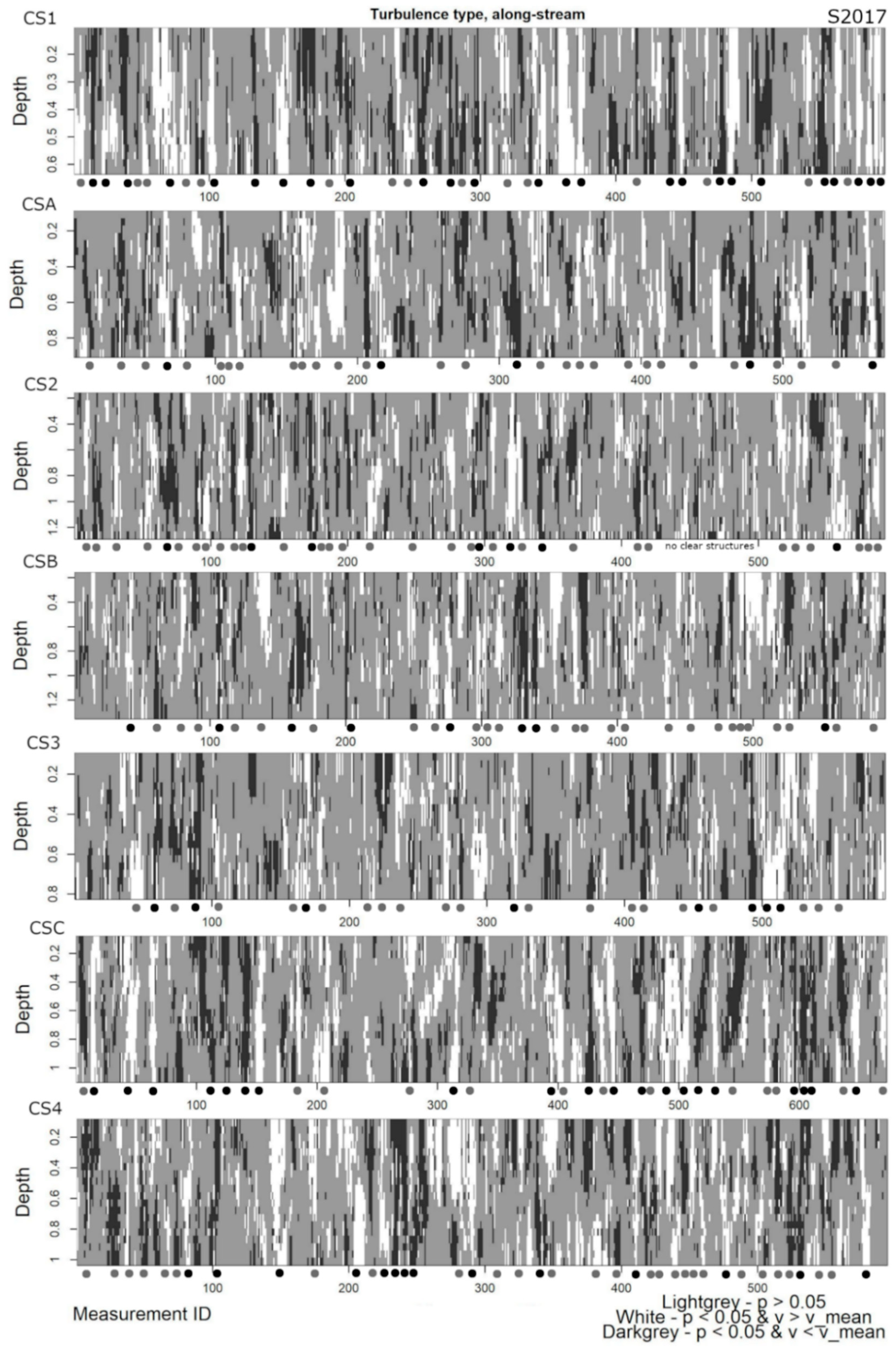
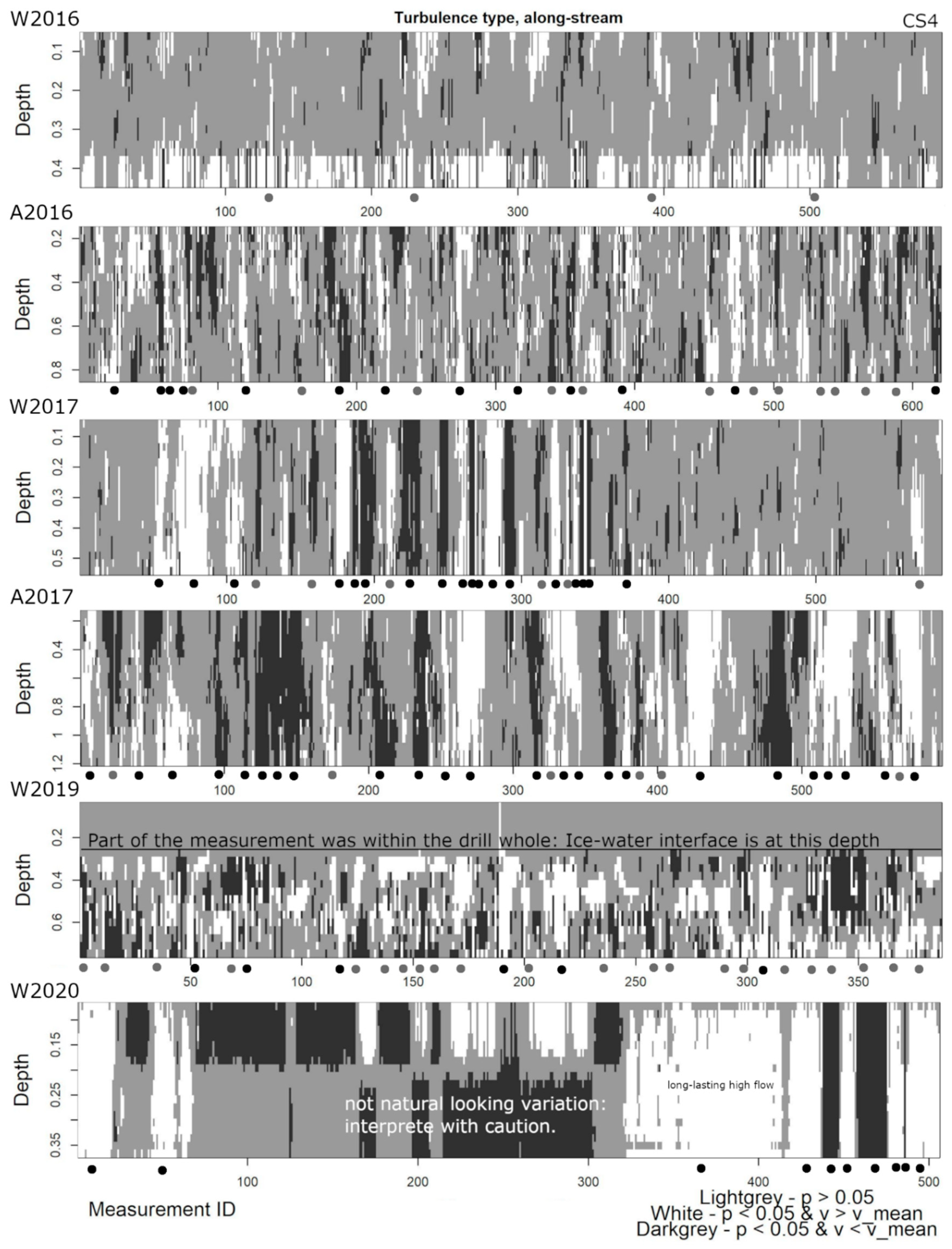
4.2. Marco-Turbulence Patterns

Based on the preliminary data check and the analyses of depth-averaged velocity, the CS1 (inlet area), CSB (apex), and CS4 (outlet area) were selected for the most detailed analyses. These locations showed the most prominent differences in flow characteristics between measurement times. In addition, when all measurement locations were analyzed, macro-turbulence was formed predominantly (W2018, Table 1) in ice-covered conditions and when the open-channel conditions had the highest discharge (S2017, Table 1), i.e., when it differed the most from the ones analyzed in [9]. Note that the discharge of S2016 and S2018 would have been even higher, but there was no good quality data available from all measurement locations during those time steps. The figures of raw streamwise (i.e., along-stream) and vertical velocities of the selected measurement times and locations are included as the Supplementary Material (see Figures S3–S10). In addition, the macroturbulent flow analyses results (LISA) based on vertical flow velocity have been included as Supplementary Material (see Figures S11 and S12). All analyzed data sets reached a good signal-to-noise ratio (SNR) of at least 5 dB [9].

4.2.1. Spatial Variation of Macro-Turbulence under Ice-Covered Conditions

The W2018 results are presented as an example of ice-covered flow condition from all measurement locations. Overall, during ice-covered conditions, the high velocity core was located in the middle of the water column, and not within the surface layer (Figures S3–S8). The streamwise (along-stream) velocity and vertical velocity data of W2018 revealed pulses of higher flow (Figures S3 and S4). These pulses reached through the whole water column, from surface to the near-bed layers. The inlet area had high streamwise velocities of 0.6–0.8 m/s during the pulses, and lower flow of 0.4–0.5 m/s occurred between them. The velocities reduced approaching the apex (CSB), and highest streamwise velocities reached approximately 0.4 m/s in the middle layers of the vertical water column. The flow velocities were also lower in the outlet area (CS4) than in the inlet area. The high flow wedges of CS4 constituted 0.3–0.4 m/s streamwise velocities, and the low flow between them was around 0.2–0.3 m/s. The vertical velocities were very low, approximately 0 m/s. However, only at the CS1 measurement location was a clear downward vertical flow observed at the surface layers of the water column. This was not observed clearly at any other measurement locations (Figure S4).
The statistically significant high and low flow velocity clusters were clearly apparent from the measurements of W2018 (Figure 3, Table 5 and Table 6). Even though the streamwise strong (i.e., unbroken) low flow wedges (n = 5), reaching from surface layers to near-bed layers, outnumbered the strong high flow wedges (n = 4), the weaker wedges (which were broken by couple of cells in vertical direction) of high flow greatly outnumbered (n = 9) the weak low flow wedges (n = 3) at CS1 location. Both strong and weak macro-turbulent flow wedges were the most equally spaced at this inlet area during W2018 measurement time. The statistically significant flow wedges, which reached from the surface to riverbed, occurred in CSA also, but those were temporally shorter, being only 1–2 s long, than at the CS1, where 4–5 s long wedges occurred. Least strong wedges occurred at CSC and CSB at that time, and the statistically significant high and low flow clusters were only near the riverbed and ice-water interface layer. Thus, the statistically significant clusters did not reach clearly through the water column. Within the apex area (from CS2 to CSC), the detection of those wedges was overall more difficult as the statistically significant high and low flow areas varied there more randomly. At those measurement locations, there was often either high or low flow cluster at the surface layer, and then the opposite clusters (i.e., low or high flow cluster) at the near-bed layer. However, at the CS4 the macro-turbulence was again more visible, and temporally wider clusters of statistically significant high and low flow wedges appeared. The strong and weak high flow wedges outnumbered the low flow wedges at CS4. Thus, based on the streamwise flow, the macro-turbulence was the clearest at the inlet area, second clearest at the outlet area, and less clear in the apex measurement locations during the mid-winter ice-covered, mostly pressurized (Table 3), low flow conditions.
The statistically significant high and low flow wedges were also seen from the vertical velocity data of W2018 (Figure S11, Table 6). Similar to the streamwise velocity, it was the clearest in the inlet area (CS1) during that measurement time, and the least visible at the apex area (from CS2 to CSB). Different to the streamwise velocity is that the vertical significant flow clusters started to appear again right after the apex at CS3 and CSC. However, in measurement locations CSA–CS4 the statistically significant vertical high and low flow vertical wedges were shorter in time than at CS1 (Figure S11).

4.2.2. Spatial Variation under Open-Channel Conditions

The S2017 measurements were used as an example of the open-channel flow conditions at each measurement location. The highest velocities of S2017 of each measurement location were closer to the water surface than the middle layers of the water column, which was the case in ice-covered flow conditions of W2018 (see Figures S3 and S5). When compared to the ice-covered flow conditions of W2018, the macro-turbulence in S2017 was more frequent and obvious in the open-channel flow conditions. The streamwise velocity values of CS1 showed that there was multiple high flow wedges of ~0.75–0.8 m/s, which were separated with lower flow (~0.5–0.6 m/s) periods (see Figure S5). Note that when the streamwise velocity was high, often then the downward vertical velocities were high (see Figures S5 and S6). The vertical flows formed two layers on S2017 at the CS1, CSA, and CS2: there was clearly downward motion within the top section of the water column, and close to zero flow conditions or slightly upward flow within the bottom section of the water column. In winter (W2018) this phenomenon had been seen only at the CS1. Overall, the vertical velocities were slow in S2017 and the main direction of the flow was streamwise (Figures S5 and S6).
In total, there were 25 statistically significant strong flow wedges at the inlet area (CS1) during 10 min-long measurements, out of which 13 were the high flow wedges (Figure 4, Table 5 and Table 6). Thus, on average there were 2–3 strong flow wedges per minute. This is a much higher frequency than encountered during any of the winter period measurements (Table 5 and Table 6). In addition, at all other measurement locations, the occurrence of both strong and weak macro-turbulent wedges was more frequent on S2017 than W2018. Only at the CSA location was there one more strong high flow wedge on W2018 than on S2017, but the weak high flow wedges also outnumbered the winter conditions at that measurement location. However, when moving from the inlet to the apex area (CS2–CS3), similar changes in the characteristics of the statistically significant high and low flow wedges appeared in S2017 as in W2018 (Figure 3 and Figure 4). The wedges became temporally narrower, (i.e., only a couple of seconds long in the apex area). In addition, the wedges became more broken. There was either high or low flow cluster at the surface layer, and then the opposite clusters (i.e., low or high flow cluster) at the near-bed layer in many occasions. This can be seen from the occurrence of the strong streamwise high and low flow wedges, whose numbers dropped, at the same time when the weak wedge numbers increased (Table 7). However, at the CSC and CS4, the streamwise flow wedges were again more obvious throughout the water column. The numbers of strong high flow wedges increased again closer to the frequencies of the inlet area’s CS1 measurement location (CSC had 11 and CS4 had 8 strong high flow wedges; see Table 7). Thus, based on this, the macro-turbulence was the clearest at the inlet area, second clearest at the outlet area, and least clear in the apex measurement locations during the open-channel conditions of spring 2017.
Similar to the macro-turbulence observed based on the streamwise velocities, it was also more frequent on S2017 than on W2018 measurement time based on vertical velocities (Figure S12, Table 7). The statistically significant high and low flow clusters did not vary much between the different parts of the bend. Therefore, the vertical zero, upward and downward flow formed statistically significant temporal clusters more consistently throughout the bend in open-channel conditions of S2017, than in ice-covered conditions of W2018.

4.2.3. Macro-Turbulence at the Meander Bend Inlet Area

The CS1, CSB, and CS4 were analyzed in more detail from all the measurement times, but only based on the streamwise velocities, as the W2018 and S2017 showed that the flow velocities were greatest in streamwise direction and the vertical flow was predominantly around 0 m/s. At the inlet (CS1), the statistically significant high and low flow wedges were less frequent during all other mid-winter measurement times than on W2018 (Figure 5). At the inlet area, least occurrences of macro-turbulence (from all measured ice-covered conditions) was observed on W2019, with only one weak high flow wedge and two weak low flow wedges. Thus, throughout the measurement, there was always at least a one or two cell gap in the wedges so that they did not reach throughout the water column. When detecting the raw velocity data sets (Figure S7), the velocities were similarly high during other winters as on W2018. For example, on W2016, approximately 0.7–0.75 m/s streamwise velocities, which reached from the surface to the near-bed layers, occurred and lower velocities of 0.5–0.6 m/s appeared between these times of high flow wedges (see Figure S7).
When open-channel conditions of CS1 were compared, the macro-turbulence was apparent during low flow conditions of A2016 (6.34 m3/s) and A2018 (3.69 m3/s), and during high discharge conditions of S2016 (Figure 6 and Figure S8). Note that in these A2016 and A2018 measurement time steps, both high and low flow wedges lasted longer in time, than in S2017, which had higher discharge condition at ~11 m3/s. Thus, the overall macro-turbulent motion of the fluid took longer to pass by the measurement point, possibly due to the overall lower discharge and the flow depths of the autumn measurement times. In S2016, multiple turbulent wedges occurred consecutively, and resulted in temporally longer high flow periods. Despite the turbulent wedges taking longer in the shallower depth conditions, the highest velocities of these flow wedges were around 0.6–0.7 m/s on S2016, A2016, and A2018 (Figure S8). Thus, these magnitudes were similar to the ice-covered conditions of W2018 and open-channel conditions of S2017, previously discussed. Thus, when the strongest statistically significant high flow wedges occurred at the inlet area of the meander bend, the streamwise flow velocity magnitudes were similar, despite the season in question. This verifies that the statistically significant flow variation throughout the vertical water column occurred at the inlet area during every season, whether being high spring or low autumn and winter flow, or whether being ice-covered pressurized (W2016, W2017, W2018: see Table 3) or non-pressurized (W2020, see Table 3) conditions.

4.2.4. Macro-Turbulence at the Meander Bend Apex

As the W2018 and S2017 data sets are already shown, the CSB measurement location representing the apex area had most often chaotic and unclear occurrence of the statistically significant high and low flow wedges. In addition to W2018 and S2017, there was also on A2016 and W2017 frequent statistically significant clusters of high and low flow either close to the riverbed or the water surface (Figure 7). Thus, these clusters of CSB did not reach through the water column.
However, exceptions were W2016, W2019, S2019, and W2020, when strong wedges of either high or low streamwise velocities occurred throughout the water column (Figure 7 and Figure S9). Especially interesting is that on W2016 and W2019 the macro-turbulence was not frequent at the inlet areas (CS1 measurement location) but was more detectable at the apex area (CSB).
The streamwise velocities were high on W2016, A2016, and A2017, reaching 0.8 m/s during the high flow pulses (Figure S9). During W2019, S2019, and W2020 measurement times, when the flow velocities were overall slow (Figure S9), the statistically significant high and low flow clusters reaching from the surface to the riverbed were longer in temporal scale (Figure 7), than during the measurement times having overall higher flow magnitudes.

4.2.5. Macro-Turbulence at the Meander Bend Outlet Area

The statistically significant high and low flow wedges were apparent at the outlet area on A2016, W2017, and A2017 measurement times. During W2017 the strong high flow clusters occurred 10 times within the 10 min-long measurement of CS4 (Table 6) and were thus more frequent than in the inlet or apex areas. The velocities of the high flow wedges at CS4 during A2017 measurement time were around 0.5 m/s (Figure S10). On A2016, the high flow pulses had 0.6–0.7 m/s streamwise velocities, which were similar to the velocities of the inlet areas, when the clearest macro-turbulent flow wedges occurred. Thus, CS4 also experienced these statistically significant high and low flow wedges during both open-channel and ice-covered seasons.
The flow structures of W2019 and W2020 differed from other measurements done at CS4, and also from other measurement locations (Figure 5, Figure 6, Figure 7 and Figure 8). The streamwise flow was more chaotic on W2019, even though the statistically significant strong high flow wedges were more frequent than at the inlet area (Table 6). The streamwise flow magnitudes were also slow throughout the measurement of W2019 (Figure 8 and Figure S10): the highest flow clusters were then only 0.3–0.4 m/s and slowest flow velocities were 0–0.2 m/s. These were reflected in the statistically significant autocorrelation areas. Similarly, the streamwise velocities of W2020 were between 0–0.2 m/s most of the time, and only a few times were close to 0.4 m/s (Figure S10). These low flow magnitudes could have caused the fact that most of the cells had statistically significant autocorrelation with neighboring cells during that measurement time (Figure 8).

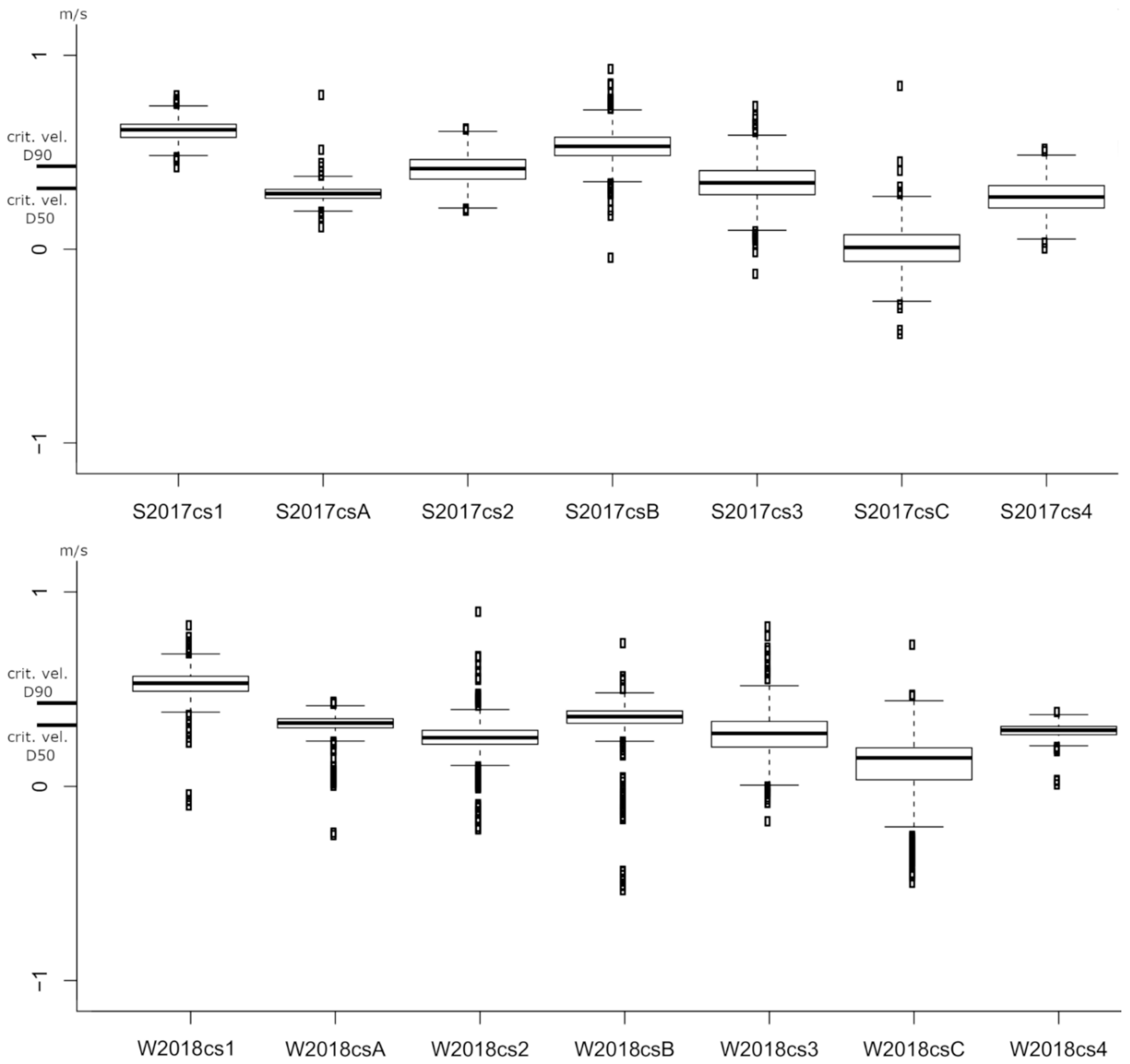
4.3. Sediment Transport and Exceedance of the Critical Velocity Thresholds for Incipient Motion

4.3.1. Measured Sediment Transport

The bedload was greatest at the CS4 measurement location on W2020, and second greatest at CS1. At CS4 the bedload was from 844.3 to 2697.4 mg/(m·s), depending on the measurement. At CS1 the bedload was from 76.8 to 391.1 mg/(m·s). Minimal transport was at CS2 and CS3, as their every sample was below 50 mg/(m·s) on 6 February 2020. Only one sample, CS2 HS1 was smaller (12.8 mg/(m·s)) than the one measured in 2017 February (22.8 mg/(m·s)). The sample “CS1 HS3” was medium sand, moderately well sorted, coarse skewed, and mesokurtic, according to the calculations done with Gradistat software [25]. The “CS4 HS1” sample was defined as coarse sand, moderately well sorted, symmetrical, and mesokurtic.
As mentioned in Section 3, each bedload sample was measured within 6 min, but not at the same time with the ADCP measurements to avoid disturbance to the flow measurement data. While it was not possible to define the effect of exact macro-turbulent flow wedges during separate bedload measurements, it was possible to show variability between the samples, which indicates differing flow conditions at each bedload measurement time.
Total suspended solids varied 0–0.5 mg/L on W2019, were 0 mg/L on A2018 and on W2018, varied 6.5–7.5 mg/L on 25 May 2018, and were again 0 mg/L on A2017 (Table 6). Therefore, the transport method was mainly bedload at the Pulmanki River during the ADCP measurement times, both during the ice-covered and open-channel conditions. Water color values and turbidity were also low during each measurement time (Table 6). The color of the water was between 20 and 50 mg/L Pt, and turbidity 0–4 FTU. The samples represented the conditions described by the ADCP data and did not include spring snow-melt discharge peak conditions.

4.3.2. Near-Bed Velocities: Exceedance of the Critical Velocity Threshold

The near-bed fluctuation at each measurement time was compared against the critical velocity threshold of sediment movement, and to the overall macro-turbulent flow characteristic of those measurement times. Based on the exceedance of the critical velocity threshold of the near-bed layer velocities, most prone conditions for riverbed erosion were at CS1 on S2017 (Figure 9, Figure 10 and Figure 11), when also the occurrence of the strong macro-turbulent flow wedges was the highest at the inlet of the meander bend (Table 6). Second- and third-highest sensitivity was on W2018 and W2016, respectively, when also pulsating flow was clear and the occurrence of the strong macro-turbulent wedges was its highest of the winters (Table 6). The streamwise velocity fluctuated much during W2016, S2016, A2016, and W2017, in that the velocities varied above and below the critical threshold of incipient motion of D90 grain sizes. Note that conditions at these times were either ice-covered low flow situations or autumn low flow situations. On W2020 there was great fluctuation above and under the threshold, with overall flow magnitudes lower than those observed on W2016 and W2017. During the winter measurements there were greater low velocity outliers within the boxplot calculations (Figure 10 and Figure 11) than during the open-channel flow situations at CS1, indicating the importance of high flow wedges for the exceedance of the critical sediment transport thresholds. The streamwise velocity of the near-bed layer would not have exceeded the critical velocity to move the D90 particles on W2019 and S2019 flow conditions at CS1. The D50 particle sizes would not have started moving on W2019 and S2019, and the threshold of the erosion would have exceeded on W2020 only occasionally (Figure 9, Figure 10 and Figure 11).
The streamwise near-bed velocities were also high at CSB, in particular on W2016 and A2017. The critical velocity threshold of D90 value of “CS4 HS1” sediment sample was exceeded within the 25–75 percentile ranges of those measurements (Figure 11). On W2016 there were few measurement time-steps when D90 would not have moved. On A2016, S2017, and S2019 the D50 and D90 thresholds were exceeded during most of the samples. Fluctuation above and below the threshold was greater than on A2017 and W2016, as during A2017 and W2016 the near-bed velocities were mostly above the threshold. Most fluctuation of the velocities above and below the D50 threshold was on W2017, as the 25–75 percentile region was around the D50 threshold velocity values (Figure 11). However, on that time, the occurrence of macro-turbulent wedges was low (Table 6). Thus, this indicates that the fluctuation of near-bed velocities at the apex was not that year related to the macro-turbulent flow wedges. The widest ranges of the outliers were on W2019 where the overall median velocity was below the D50 threshold. That same period, similar to W2017, the macro-turbulent wedges were low at this apex area (Table 6). During that low flow period the fluctuation of the flow magnitude was the greatest for the initiation of the sediment transport. On W2020, the median velocities were below the critical thresholds for the incipient movement, and the outlier ranges were also smaller than on W2019 at CSB. Thus, least prone conditions for erosion were on W2020 at CSB.
At CS4, the critical velocity was exceeded most frequently during A2016, when a great amount of strong macro-turbulent flow wedges had occurred (Table 5). The D50 threshold was frequently exceeded on W2016, W2017, W2018, S2017, and A2017. These all had multiple macro-turbulent flow wedges, except on W2016 (Table 6). Thus, during most of those periods the flow pulses caused the exceedance of the threshold. However, the velocities measured on W2019 and W2020 basically did not exceed the critical threshold of streamwise velocity and the statistically significant flow wedges had overall slower velocities than in other years. On W2020, when the “CS4 HS1” sample had been measured, the outlier negative (i.e., towards upstream), near-bed velocity values exceeded the D50 grain size threshold. At other measurement locations, there were several time steps (outlier values of the boxplots), where the upstream velocities were high enough that the movement of both D90 and D50 particles of bead load sample “CS4 HS1” would have started (Figure 10 and Figure 11).
In addition, the velocity threshold for deposition of the largest analyzed D90 grain size particles (0.07 m/s) was exceeded according to the median near-bed flow velocities during most of the measurement times at CS1, CSB, and CS4 locations (Figure 9, Figure 10 and Figure 11). Only during W2019 and W2020 the flow measurement samples had near-bed velocity values often close to zero. Thus, the sediment particles, whose motion had possibly started further upstream, would not have had velocities low enough for their settlement, as the velocities were predominantly within the transport zone defined by Hjulström [24].

5. Discussion

Similarly to Lotsari et al. [2] who demonstrated based on cross-sectional measurements conducted at the Pulmanki River in 2014–2015, the high velocity core was located in the middle of the water column in ice-covered flow conditions of 2016–2020, whereas in open-channel conditions the highest velocities are located closer to the water surface than the riverbed. The winter discharges of the Pulmanki River were mostly lower than those observed by Demers et al. [9], and the spring discharges were higher. However, the autumn discharges were in similar magnitude as in the study site of Demers et al. [9]. In comparison, the study site of Demers et al. [9] had ice roughness from low relief wavy forms to high amplitude undulations with scarp faces, thus the ice cover of the Pulmanki River was smoother by comparison. Despite these differences to Demers et al. [9] overall discharge and ice-cover conditions, macro-turbulence was observed at the Pulmanki River. The statistically significant clusters of high and low flow were observed during all measured seasons and locations within a symmetrical meander bend. However, there were also periods where the statistically significant high flow clusters were weaker and were “broken” in the middle of the vertical water column so that these wedges had a short gap between the surface and bottom layers of the water column. Particularly within the apex area, these clusters were sometimes difficult to define and some of the statistically significant flow areas were left outside of the frequency calculations if they occurred predominantly in the bottom half of the water column or top half of the water column. These types of clusters occurred both in open-channel and ice-covered conditions.
According to Sukhodolov et al. [11], periods of bursting flow (i.e., ejection events can be identified as periods when vertical velocity is greater than 0 and streamwise velocity is less than 0) and periods of sweep events occur when streamwise flow is greater than 0 and vertical velocity is less than 0. In addition, it has been observed that the vertical ejections would be able to reach throughout the water column, but sweeps are said to reach up to 0.7–0.8 times the river depth [9]. As the streamwise velocity was mostly positive (downstream) at the Pulmanki River, this indicates that the bursting ejections were not occurring (i.e., vertical flow was directed seldomly towards the surface at Pulmanki River) during the strong streamwise flow wedges. As the sweeps are defined to reach only up to 0.7–0.8 times the river depth [9], these bursting sweeps could influence the weak macro-turbulent flow structures. However, similar to Demers et al. [9], the length of the vertical stripes of coherent flow structures, reaching from the surface to the riverbed, were longer than the sampling frequency. Therefore, these strongest coherent flow structures occurred quasi-steadily and met the criteria of the macro-turbulent flow [9], and not only bursting ejections and sweeps at the channel bed or at the surface air-water/ice-water interfaces [11].
During ice-covered conditions, these statistically significant high and low flow wedges occurred most consistently in the upstream inlet area (CS1), and secondly at the outlet area (CS4). The flow pulsation was significant in the inlet area, where the water depth was also shallow under ice. There was more variability in flow velocities at the apex, and it was not possible to see clear macro-turbulent flow pulsation in these high velocity measurement locations close to the outer bank. Thus, the pattern of flow in the inlet area was similar to Demers et al. [9]. The riffle in the inlet area of the Pulmanki River could explain the macroturbulence, much like Marquis and Roy [7] stated. However, as we did not have measurements from the upstream riffle-pool section (i.e., further upstream of the CS1 measurement location), we cannot state this for sure. Note that during ice-covered flow, only at this inlet area was there a clear layer of downward flow, indicating that there was circulating cells in the vertical direction, in addition to the streamwise macro-turbulent pulsating flow to the downstream direction. This vertical circulation cell could indicate the conditions also observed by Shvidchenko and Pender [6] in their flume study. These authors observed an upward flow in the bottom layer of the water column and a downward flow in the top layer of the water column due to macro-turbulence.
Macro-turbulence was observed during the open-channel flow conditions in autumn and spring. Similar to the ice-covered conditions, the occurrence of the high and low flow pulses was the most consistent at the inlet (CS1) and then secondly at the outlet of a meander bend (CS4). More variable and chaotic nature of the flow velocities was observed in the apex area. Macro-turbulence occurred the most frequently at the inlet area in spring 2017, which had one of the highest discharges of the 5–10 min-long ADCP measurement times. These statistically significant strong (i.e., vertically unbroken) flow wedges reaching from the surface to the near-bed layers occurred 2–3 times per minute, in addition to the occurring weaker (i.e., broken within 5–20% of the depth of the measurement time) statistically significant flow clusters. This is far from the frequency observed by Buffin-Bélanger et al. [5], who observed the more than two second-long large-scale flow structures to occur up to nine times per minute. Similar to the ice-covered period, in spring open-channel high flow conditions (e.g., S2017), the vertical velocity was observed to be downwards at the surface layers within the inlet area (CS1) and at the two following cross-sections closer to the apex (CSA and CS2). Thus, the vertical flow circulation was similar to Shvidchenko and Pender [6] also during the spring open-channel discharge conditions of the Pulmanki River.
Despite the frequency of the strong flow wedges was not as consistent and frequent during other measurement times than on S2017 at the Pulmanki River, the clearest statistically significant high flow wedges had always streamwise velocities at least 0.6–0.7 m/s, independently of the season. One difference between the seasons was that the strong statistically significant flow wedges were temporally longer during the measurement times, when the overall discharge was slower. This was especially the case in the inlet and outlet areas of the meander bend. Thus, our results show similarities to a previous study [9] in the sense that the time and length scales were larger for the ice-covered flow situation than the open-channel flow conditions.
Buffin-Bélanger et al. [5] noticed that the macro-turbulent flow cells were tilted towards downstream, in that the average angle of the front of the wedges was 36°. Despite the high velocity wedges occasionally being tilted at the Pulmanki River, they were mostly straight from surface to the bottom layers of the flow. Thus, we were not able to see this consistent tilting from the ice-covered and open-channel flow data of ours. Note that the depths of Buffin-Bélanger et al. [5] were mostly less than 30 or 20 cm (i.e., much smaller than the ones of this present study; Table 2 and Table 3).
The apex area differed from the inlet and outlet areas in regards to the characteristics of the statistically significant flow clusters during ice-covered low flow (winter), open-channel high flow (spring), and open-channel low flow (autumn) conditions. The macro-turbulent flow wedges were the weakest and temporally shortest (i.e., only 1–2 s long) in the apex region (CS2–CSC). In the inlet areas the 4–5 s long wedges corresponded to the lengths of Demers et al. [9], who stated that the macro-turbulent flow wedges in streamwise velocity direction were in ice-covered conditions 0.4 times the depth. Thus, the apex area of Pulmanki River’s bend had temporally shorter macro-turbulent flow structures than Demers at al. [9] observed. During S2017 measurement time, for example, when moving from inlet to the apex region, the numbers of the strong streamwise high and low flow wedges dropped, at the same time the weak wedge numbers increased. In addition, many statistically significant high and low flow clusters appeared often either near the riverbed or near the surface (ice-water/air-water interface) layer at the apex. There were also frequent high flow clusters at the surface layers, and low flow clusters simultaneously near the riverbed, or vice versa. Thus, the statistically significant clusters did not reach through the water column, and this turbulence was possibly caused by the friction effect of both the riverbed and ice-cover and not the actual macro-turbulence. It could have also been partially caused by the centrifugal forces and the friction caused by the outer bank. Unique to many other measurement times were W2016 and W2019 measurements, as during those times the statistically significant flow wedges reaching from the surface to the riverbed were not frequent at the inlet areas (CS1 measurement location), but were more detectable at the apex area (CSB). Due to the less frequent macro-turbulence at the inlet area, we suggest that the turbulence at the apex area was that time caused by local friction and centrifugal forces and not the macro-turbulence.
According to Shvidchenko and Pender [6], these depth-scale eddies are an important turbulence mechanism contributing to sediment transport, as they cause longitudinal troughs and ridges on bed and cause transport of particles along troughs. The data sets showed that the critical velocities for incipient motion were exceeded in both ice-covered and open-channel conditions. The most prone velocity situation for erosion, based on the exceedance of the critical velocity threshold of the near-bed layer streamwise velocities, was at CS1 on S2017 and second- and third-highest sensitivity were on W2018 and W2016, respectively, when variation of high and low near-bed streamwise flow velocities was also clear. The near-bed streamwise velocity fluctuated greatly during W2016, S2016, A2016, and W2017 (i.e., the velocities varied above and below the critical threshold of incipient motion of the sediment grain sizes of Pulmanki River). The macro-turbulence thus enabled the exceeding of the thresholds during these low flow open-channel and ice-covered conditions when the overall discharges were small. However, note that in addition to the existence of the macro-turbulent flow wedges, also local near-bed turbulence due to friction caused the threshold for incipient motion to be exceeded. There were spatial differences between the inlet, apex, and outlet areas, whether the threshold for motion was exceeded. The thresholds for D50 particle sizes to move were exceeded at CS1 during most of the measurement times, second often during different seasons at the apex (CSB), and most seldomly at the outlet area (CS4). However, at CSB the highest fluctuations of near-bed velocities occurred, when there was not as much macro-turbulent flow. This indicates that the small scale turbulence near the channel bed was the cause of the transport at the apex area. In addition, the highest near-bed velocities were not detected at the same measurement time at the inlet, apex, and outlet areas. This could be also due to the different depth and bedform conditions of the river channel related to the measurement times. In any case, when the macro-turbulent wedge frequencies, and the bedload amounts were compared together, the bedload transport was the greatest at CS4 and CS1, which also had the most macro-turbulent wedge occurrences (both in number, and per minute). Thus, similar to the results of previous studies on open-channel flow conditions [5,6,7,8], the macro-turbulent flow is an important contributor to sediment transport, such as that observed at the inlet and outlet of the meander bend at the Pulmanki River. However, our results show that it is especially important during low flow situations when the overall velocities and discharges are not high.

6. Conclusions

Macro-turbulent flow wedges were observed in every measurement location at the meandering Pulmanki River during ice-covered low flow conditions and open-channel flow conditions. Pressurized winter-time conditions were not a requirement for the development of the macro-turbulent flow.
These macro-turbulent flows occurred most consistently, based on the streamwise velocities, in the inlet area and second most often in the outlet area of the meander bend during both ice-covered and open-channel conditions. Centrifugal forces and local friction due to confining channel and river ice surface could have caused chaotic flow pattern at the apex. Thus, the macro-turbulent flow structures were not clear in the apex area of the analyzed meander bend.
In line with previous studies, the temporal length of the macro-turbulence was longer in conditions of low discharges and shallow depths, than in high discharge conditions. However, the longest statistically significant high flow wedges occurred at inlet and outlet areas and were temporally shorter around the apex. The frequency of the macro-turbulence was the greatest during the spring open-channel conditions. However, similar to all seasons, clearest and strongest macro-turbulent high flow wedges had velocities of at least 0.6–0.7 m/s.
Despite near-bed velocity fluctuation and the macro-turbulent flow contributing to the sediment transport during the high discharge periods, during those measurement times the overall velocities were high, and therefore the macro-turbulence was not as critical to the sediment transport as during lower discharge conditions. There were spatial differences between the inlet, apex, and outlet areas, where the critical velocity threshold for sediment movement was exceeded by the near-bed streamwise velocities. The threshold was exceeded often at the inlet, where the statistically significant macro-turbulent flow wedges occurred the most consistently. Thus, the macro-turbulence was especially important for initiation of bed sediment movement during low flow situations (i.e., when the overall velocities were not high). The macro-turbulence enabled the flow velocities to exceed the sediment movement threshold more often than based on solely the turbulence caused by the friction of the riverbed.

Supplementary Materials

The following are available online at https://www.mdpi.com/2073-4441/12/7/1874/s1. R package folder S1: S1_adcp_R_package_windows_computer; R package folder S2: S2_adcp_R_package_linux_computer; Figure S3: S3_W2018_streamwise_velocity; Figure S4: S4_W2018_vertical_velocity; Figure S5: S5_S2017_streamwise_velocity; Figure S6: S6_S2017_vertical_velocity; Figure S7: S7_CS1_streamwise_velocity_winters; Figure S8: S8_CS1_streamwise_velocity_openchannel_conditions; Figure S9: S9_CSB_streamwise_velocity; Figure S10: S10_CS4_streamwise_velocity; Figure S11: S11_LISA_W2018_vertical_velocity; Figure S12: S12_LISA_S2017_vertical_velocity. The raw ADCP data sets were opened via Zenodo: ADCP data of ice-covered and open-channel (macro-turbulent) flow, Pulmanki River, 2016-2020; ADCP_data_Lotsari_et_al_Water_opened.zip; DOI: 10.5281/zenodo.3855035.

Author Contributions

Conceptualization, E.L.; data curation, E.L.; formal analysis, E.L. and M.D.; funding acquisition, E.L., M.K., P.A., and E.K.; investigation, E.L. and M.D.; methodology, E.L. and M.D.; project administration, E.L.; software, M.D.; validation, E.L. and M.D.; visualization, E.L. and M.D.; writing—original draft, E.L.; writing—review and editing, E.L., M.D., M.K., P.A., and E.K. All authors have read and agreed to the published version of the manuscript.

Funding

This work was supported financially by the Academy of Finland (ExRIVER, grant number: 267345; InfraRiver: 296090), the Maj and Tor Nessling Foundation (ExRIVER, grant numbers: 201300067 and 201500046; Influence of river ice and fluvial processes on river environments now and in the future, grant number: 201600042) and Strategic Research Council at the Academy of Finland (Competence-Based Growth Through Integrated Disruptive Technologies of 3D Digitalization, RobotiCS, Geospatial Information and Image Processing/Computing – Point Cloud Ecosystem, grant number: 293389). In addition, the Department of Geographical and Historical Studies, University of Eastern Finland, supported the work financially.

Acknowledgments

The authors would like to thank Mariana Verdonen, Tiia Tarsa, and Marko Kärkkäinen from the University of Eastern Finland, William Speirs (at that time) from the University of Queensland (Brisbane, Australia), and Linnea Blåfield, Jouni Salmela, and Tua Nylén from the University of Turku for their valuable fieldwork assistance during 2016–2020. It would not have been possible to conduct the fieldwork without the drilling assistance of Ilkka Syvänperä and Esa Karpoff from the Kevo Subarctic Research Institute of University of Turku during 2016–2020. M.Econ. B.Eng. William Speirs (with a background in water engineering, current affiliation: Urban Utilities, Brisbane, Australia) is also thanked for checking the English language of the paper.

Conflicts of Interest

The authors declare no conflicts of interest.

References

  1. Demers, S.; Buffin-Bélanger, T.; Roy, A.G. Helical cell motions in a small ice-covered meander river reach. River Res. Appl. 2011, 27, 1118–1125. [Google Scholar] [CrossRef]
  2. Lotsari, E.; Kasvi, E.; Kämäri, M.; Alho, P. The effects of ice cover on flow characteristics in a subarctic meandering river. Earth Surf. Process. Landf. 2017, 42, 1195–1212. [Google Scholar] [CrossRef]
  3. Lotsari, E.; Tarsa, T.; Kämäri, M.; Alho, P.; Kasvi, E. Spatial variation of flow characteristics in a subarctic meandering river in ice-covered and open-channel conditions: 2D hydrodynamic modelling approach. Earth Surf. Process. Landf. 2019, 44, 1509–1529. [Google Scholar] [CrossRef] [Green Version]
  4. Hartung, F.; Scheuerlein, H. Macro-turbulent flow in steep open-channels with high natural roughness. In Proceedings of the 12th Congress of International Association for Hydraulic Research, vol 1 (River Hydraulics), Colorado State University, Fort Collins, CO, USA, 11–14 September 1967; Paper A1. pp. 1–8. [Google Scholar]
  5. Buffin-Bélanger, T.; Roy, A.G.; Kirkbride, A.D. On large-scale flow structures in a gravel-bed river. Geomorphology 2000, 32, 417–435. [Google Scholar] [CrossRef]
  6. Shvidchenko, A.B.; Pender, G. Macro-turbulent structure of open-channel flow over gravel-beds. Water Resour. Res. 2001, 37, 709–719, paper number: 2000WR90028. [Google Scholar] [CrossRef]
  7. Marquis, G.A.; Roy, A.G. From Macro-turbulent flow structures to large-scale flow pulsations in gravel-bed rivers. In Corerent Flow Structures at Earth’s Surface; Venditti, J.G., Best, J.L., Church, M., Hardy, R.J., Eds.; Joh Wiley & Sons: Chichester, UK, 2013; 387p. [Google Scholar] [CrossRef]
  8. Wohl, E. Rivers in the Landscape, 2nd ed.; John Wiley & Sons: Hoboken, NJ, USA; Chichester, UK, 2020; 535p. [Google Scholar]
  9. Demers, S.; Buffin-Bélanger, T.; Roy, A.G. Macroturbulent coherent structures in an ice-covered river flow using a pulse-coherent acoustic Doppler profiler. Earth Surf. Process. Landf. 2013, 38, 937–946. [Google Scholar] [CrossRef]
  10. Baker, V.R. Paleohydraulics and hydrodynamics of scabland floods. In The Channeld Scabland: A Guide to the Geomorphology of the Columbia Basin, Washington, Proceedings of the Prepared for the Comparative Planetary Geology Field Conference held in the Columbia Basin, USA, 5–8 June 1978; Baker, V.R., Nummedal, D., Eds.; Planetary Geology Program, Office of Space Science, National Aeronautics and Space Administration: Washington, DC, USA, 1978. [Google Scholar]
  11. Sukhodolov, A.; Thiele, M.; Bungartz, H.; Engelhardt, C. Turbulence structure in an ice-covered, sand-bed river. Water Resour. Res. 1999, 353, 889–894. [Google Scholar] [CrossRef]
  12. Willmarth, W.W.; Lu, S.S. Structure of the reynolds stress and the occurrence of bursts in the turbulent boundary layer. Adv. Geophys. 1975, 18 Pt A, 287–314. [Google Scholar]
  13. Lotsari, E.; Vaaja, M.; Flener, C.; Kaartinen, H.; Kukko, A.; Kasvi, E.; Hyyppä, H.; Hyyppä, J.; Alho, P. Annual bank and point bar morphodynamics of a meandering river determined by high-accuracy multitemporal laser scanning and flow data. Water Resour. Res. 2014, 50, 5532–5559. [Google Scholar] [CrossRef]
  14. Kasvi, E.; Vaaja, M.; Alho, P.; Hyyppä, H.; Hyyppä, J.; Kaartinen, H.; Kukko, A. Morphological changes on meander point bars associated with flow structure at different discharges. Earth Surf. Process. Landf. 2013, 38, 577–590. [Google Scholar] [CrossRef]
  15. Kämäri, M.; Alho, P.; Colpaert, A.; Lotsari, E. Spatial variation of river-ice thickness in a meandering river. Cold Reg. Sci. Technol. 2017, 137, 17–29. [Google Scholar] [CrossRef]
  16. Sontek. RiverSurveyour–Discharge, Bathymetry and Current Profiling. Brochure; Sontek: San Diego, CA, USA, 2015. [Google Scholar]
  17. Yorke, T.H.; Oberg, K.A. Measuring river velocity and discharge with acoustic Doppler profilers. Flow Meas. Instrum. 2002, 13, 191–195. [Google Scholar] [CrossRef]
  18. Beltaos, S. Hydro-climatic impacts on the ice cover of the lower Peace River. Hydrol. Process. 2008, 22, 3252–3263. [Google Scholar] [CrossRef]
  19. Turcotte, B.; Morse, B.; Bergeron, N.E.; Roy, A.G. Sediment transport in ice-affected Rivers. J. Hydrol. 2011, 409, 561–577. [Google Scholar] [CrossRef]
  20. R Development Core Team. R: A Language and Environment for Statistical Computing [Computer software manual]. Vienna, Austria, 2020. Available online: http://CRAN.R-project.org (accessed on 12 May 2020).
  21. Anselin, L. Local indicators of spatial association—LISA. Geogr. Anal. 1995, 27, 93–115. [Google Scholar] [CrossRef]
  22. Bjornstad, O.N. Ncf: Spatial Covariance Functions. R package version 1.2-9. 2020. Available online: https://CRAN.R-project.org/package=ncf (accessed on 12 May 2020).
  23. Helley, E.J.; Smith, W. Development and Calibration of a Pressure-Difference Bedload Sampler; U.S. Geological Survey Open-File Report; U.S. Department of the Interior; Geological Survey; Water Resources Division: Menlo Park, CA, USA, 1971; 18p.
  24. Hjulström, F. Studies of morphological activity of rivers as illustrated by the River Fyris. Bull. Geol. Inst. Univ. Upps. 1935, 25, 221–527. [Google Scholar]
  25. Blott, S.J.; Pye, K. GRADISTAT: A grain size distribution and statistics package for the analysis of unconsolidated sediments. Earth Surf. Process. Landf. 2001, 26, 1237–1248. [Google Scholar] [CrossRef]
Figure 1. The overall study site location. (A) Aerial photograph of the study site location. The measurements were done from the high velocity core location of seven cross-sections. (B,C) The location of the study site in Finland.
Water 12 01874 g001
Figure 2. The acoustic Doppler current profiler (ADCP) measurement locations of each analyzed time period. The Global Positioning System (GPS) signals of 9 September 2017 measurements at CSC and CS4 (CS = cross-section) were not as good as in other measurement times, and therefore their exact measurement locations (yellow dots) are not shown on the map. Those were measured within the point clusters of CSC and CS4 of the other measurement times. Note that the measurement times on 25 May 2016 (spring), 23 May 2018 (spring), and 8 September 2018 (autumn) are not shown, since from those times only data from CS1 location were included in the analyses (see Section 3 and Table 1), and their locations were within the cluster of other CS1 measurements. The GoPro camera photograph shows the riverbed sediment and the low undulation of the ice-water interface at the CS1 on 10 February 2018.
Water 12 01874 g002
Figure 3. The LISA analysis results at each measurement location, calculated based on along-stream (i.e., streamwise) velocity of W2018. Measurement ID means the sample numbers (n), and therefore also represents seconds. The black dots indicate the occurrence times of statistically significant strong high and low flow wedges reaching from the surface to the riverbed. The grey dots indicate the times when there is weaker wedge (i.e., a cluster has broken with a few cells within the vertical water column).
Water 12 01874 g003
Figure 4. The LISA analysis results at each measurement location, calculated based on along-stream (i.e., streamwise) velocity of S2017. Measurement ID means the sample numbers (n), and therefore also represents seconds. The black dots indicate the occurrence times of statistically significant strong high and low flow wedges reaching from the surface to the riverbed. The grey dots indicate the times when there is weaker wedge (i.e., a cluster has broken with a few cells within the vertical water column).
Water 12 01874 g004
Figure 5. The results of the LISA analysis of winters 2016, 2017, 2019, and 2020 at CS1 based on streamwise velocity. The W2018 results can be seen from Figure 3. Measurement ID means the sample numbers (n), and therefore also represents seconds. W2019 and W2020 measurements were shorter in time. The black dots indicate the occurrence times of statistically significant strong high and low flow wedges reaching from the surface to the riverbed. The grey dots indicate the times when there is weaker wedge (i.e., a cluster has broken with a few cells within the vertical water column).
Water 12 01874 g005
Figure 6. The results of the LISA analysis of open-channel conditions at CS1 based on streamwise velocity. The S2017 results can be seen from Figure 4. Measurement ID means the sample numbers (n), and therefore also represents seconds. The black dots indicate the occurrence times of statistically significant strong high and low flow wedges reaching from the surface to the riverbed. The grey dots indicate the times when there is weaker wedge (i.e., a cluster has broken with a few cells within the vertical water column).
Water 12 01874 g006
Figure 7. The results of the LISA analysis at CSB during all measurement times based on streamwise velocity. The S2017 and W2018 results can be seen from Figure 3 and Figure 4. Measurement ID means the sample numbers (n), and therefore also represents seconds. Note that the S2019 and W2020 measurements were shorter in time. The black dots indicate the occurrence times of statistically significant strong high and low flow wedges reaching from the surface to the riverbed, and the grey dots indicate the times when there is weaker wedge (i.e., cluster has broken with a few cells within the vertical water column).
Water 12 01874 g007
Figure 8. The results of the LISA analysis at CS4 during all measurement times based on streamwise velocity. The S2017 and W2018 results can be seen from Figure 3 and Figure 4. Measurement ID means the sample numbers (n), and therefore also represents seconds. Note that the W2019 and W2020 measurements were shorter in time. The black dots indicate the occurrence times of statistically significant strong high and low flow wedges reaching from the surface to the riverbed, and the grey dots indicate the times when there is weaker wedge (i.e., cluster has broken with a few cells within the vertical water column). W2019 ice-water interface is marked in the figure.
Water 12 01874 g008
Figure 9. The streamwise velocity (m/s) of the deepest cells at all measurement locations on W2018 (mid-winter ice-covered flow conditions) and S2017 (spring snow-melt flow conditions). The critical velocity thresholds for the movement of the largest measured D50 and D90 grain sizes are shown. Note that the deepest cells are at different depths depending on the measurement times.
Water 12 01874 g009
Figure 10. The boxplots of the streamwise velocity (m/s) of the deepest cells at all measurement locations on W2018 (mid-winter ice-covered flow conditions) and S2017 (spring snow-melt flow conditions). The critical velocity thresholds for the movement of the largest measured D50 and D90 grain sizes are shown. Note that the deepest cells are at different depths depending on the measurement times. The boxplots show the median line, 1st and 3rd quartiles (25 and 75 percentile ranges) within the boxes, maximum observations below upper and lower fences (i.e., the fence is 1.5 times the difference between the 3rd and 1st quartiles), and outliers (dots).
Water 12 01874 g010
Figure 11. The boxplots of streamwise velocity (m/s) of the deepest cells at CS1, CSB, and CS4 measurement locations during each measurement time. The critical velocity thresholds for the movement of the largest measured D50 and D90 grain sizes are shown. Note that the deepest cells are at different depths depending on the measurement times. The boxplots show the median line, 1st and 3rd quartiles (25 and 75 percentile ranges) within the boxes, maximum observations below upper and lower fences (i.e., the fence is 1.5 times the difference between the 3rd and 1st quartiles), and outliers (dots). In particular, scattering occurred on W2019 at CSB, as there were wide ranges in the outlier values.
Water 12 01874 g011
Table 1. The measurement times, applied sensors, discharge, and notes. In the acronyms of the measurement times W = winter (low flow period, February), S = spring (snow-melt flood period, May), A = autumn (low flow period, September). These raw ADCP data sets (Matlab format) are shared with the paper (DOI: 10.5281/zenodo.3855035). Bad quality relates to the S5 sensor malfunction.
DateAcronymSensor (Sontek)Discharge (m3/s)Notes
17 February 2016W2016M91.38 Good quality
25 May 2016S2016S512.40 Bad quality, discarded all but CS1.
10 September 2016A2016M96.34Good quality
16 February 2017W2017M91.32 Good quality
31 May 2017 S2017M910.95 Good quality
9 September 2017A2017M94.59 Good quality, except CS1 was too shallow and discarded
9 February 2018W2018M90.18Good quality
23 May 2018S2018S515.80 Bad quality, discarded all but CS1
8 September 2018A2018S53.69 Bad quality, discarded all but CS1
8 February 2019W2019M90.61 Good quality
21 May 2019S2019M96.04 Good quality, except CS4 discarded as location fluctuated
2019 Autumn ---No measurements
6 February 2020W2020M90.79Good quality
Table 2. The basic flow characteristics of each of the analyzed open-channel low measurement from their measurement location (see Figure 1 and Figure 2) within cross-sections (CS). The average, minimum, and maximum values of depth-averaged (D-A) velocities were defined. During open channel conditions, the measurement of CS1 was always conducted on the left bank side of the mid-channel bar, and the measurement of CSA and CS2 on the right bank side of the mid-channel bar.
DateParameterCS1 (Left Bank)CSA (Right Bank)CS2 (Right Bank)CSBCS3CSCCS4
S2016samples680------
average D-A velocity (m/s)0.574------
min D-A velocity (m/s)0.232------
max D-A velocity (m/s)0.791------
depth (m)0.92------
A2016samples606602661603589608620
average D-A velocity (m/s)0.5050.3400.5370.6510.4270.3020.515
min D-A velocity (m/s)0.2260.2020.3270.4180.1020.0220.287
max D-A velocity (m/s)1.1020.7540.6840.7740.7650.870.665
depth (m)0.590.921.421.591.3540.960.96
S2017samples598571592597589672595
average D-A velocity (m/s)0.6470.3550.5000.4930.3980.1010.289
min D-A velocity (m/s)0.4100.2300.3550.1900.1600.0040.124
max D-A velocity (m/s)0.7550.5870.5780.8270.7070.4920.486
depth (m)0.721.051.531.781.121.3141.43
A2017samples-608596609601598597
average D-A velocity (m/s)-0.4350.6200.6670.1220.3510.306
min D-A velocity (m/s)-0.2020.3240.4060.0020.1170.096
max D-A velocity (m/s)-0.5980.7630.7910.5050.6730.468
depth (m)-0.811.131.5641.260.911.49
S2018samples473------
average D-A velocity (m/s)0.380------
min D-A velocity (m/s)0.231------
max D-A velocity (m/s)0.561------
depth (m)1.07------
A2018samples621------
average D-A velocity (m/s)0.527------
min D-A velocity (m/s)0.67------
max D-A velocity (m/s)0.309------
depth (m)0.65------
S2019samples591299267299287364-
average D-A velocity (m/s)0.2210.3450.4180.4220.1650.257-
min D-A velocity (m/s)0.1450.2450.2100.2820.0390.065-
max D-A velocity (m/s)0.2740.4000.5800.5870.5230.450-
depth (m)0.931.281.541.730.711.20-
Table 3. The basic flow characteristics of each of the analyzed ice-covered measurements from their measurement location (see Figure 1 and Figure 2) within cross-sections (CS). The average, minimum, and maximum values of depth-averaged (D-A) velocities were defined. In some winters the CS1, CSA, and CS2 had mid-channel bars, where the ice was bottom-fast (i.e., reached the riverbed). During those winters, the channel width was measured from both sides (left and right bank) of the mid-channel bars. NMB = no mid-channel bar.
DateParameterCS1 (Left Bank)CS1 (Right Bank)CSA (Left Bank)CSA (Right Bank)CS2 (Left Bank)CS2 (Right Bank)CSBCS3CSCCS4
W2016samples663--671-677593591567590
average D-A velocity (m/s)0.570--0.408-0.5670.5140.2460.2130.256
min D-A velocity (m/s)0.356--0-0.2560.3750.0320.0120.068
max D-A velocity (m/s)0.979--1.787-1.1110.6991.0410.9070.344
depth (m)0.43--0.39-0.500.610.670.610.55
t i , i.e., ice thickness (m)0.38--0.51-0.510.480.450.400.43
width of the ice-covered channel (m)8.04NMB NMB17.99NMB5.957.578.9311.6712.72
0.0072W1.33 (see Equation (1))0.12--0.34-0.080.110.130.190.21
pressurized (P) vs. non-pressurized flow (N) (Equation (1))P--P-PPPPP
W2017samples599-567535-650673612587585
average D-A velocity (m/s)0.378-0.2610.165-0.3130.3340.2710.2350.208
min D-A velocity (m/s)0.226-0.1150.084-0.1750.2300.080.0850.106
max D-A velocity (m/s)0.532-0.3440.249-0.5510.5330.6130.5550.440
depth (m)0.48-0.410.58-0.850.990.790.530.67
t i , i.e., ice thickness (m)0.35-0.400.42-0.440.330.440.50.44
width of the ice-covered channel (m)12.842.0920.95NMBNMB8.846.98.7812.8619.01
0.0072W1.33 (see Equation (1))0.22-0.410.41-0.130.090.130.220.36
pressurized (P) vs. non-pressurized flow (N) (Equation (1))P-NP-PPPPP
W2018samples604--625-592593621577577
average D-A velocity (m/s)0.514--0.266-0.2290.3440.2990.1380.281
min D-A velocity (m/s)0.262--0.125-0.0050.0500.1580.0120.131
max D-A velocity (m/s)0.719--0.365-0.7400.7410.9420.2770.440
depth (m)0.54--0.51-0.620.350.900.560.59
t i , i.e., ice thickness (m)0.25--0.3-0.290.300.30.470.27
width of the ice-covered channel (m)13.936.974.989.045.894.98.0210.1412.3215.51
0.0072W1.33 (see Equation (1))0.24--0.14-0.060.120.160.200.28
pressurized (P) vs. non-pressurized flow (N) (Equation (1))P--P-PPPPN
W2019samples142-383--282506242315387
average D-A velocity (m/s)0.019-0.250--0.0860.0700.0510.1020.100
min D-A velocity (m/s)0.001-0.000--0.0020.0010.0040.0000.004
max D-A velocity (m/s)0.178-2.166--0.6400.8530.1941.4090.494
depth (m)0.57-0.43--0.851.011.510.890.90
t i , i.e., ice thickness (m)0.31-0.3--0.410.350.250.380.34
width of the ice-covered channel (m)121.957.923NMB9.967.996.0515.6915.91
0.0072W1.33 (see Equation (1))0.20-0.11--0.150.110.080.280.29
pressurized (P) vs. non-pressurized flow (N) (Equation (1))P-P--PPPPP
W2020samples352--322-311318353562506
average D-A velocity (m/s)0.369--0.349-0.0900.2670.2350.2710.234
min D-A velocity (m/s)0.067--0.046-0.0060.0180.0450.0040.075
max D-A velocity (m/s)0.718--2.124-0.6910.5220.6330.9120.794
depth (m)0.34--0.35-0.770.800.660.470.47
t i , i.e., ice thickness (m)0.30--0.40-0.380.360.320.350.38
width of the ice-covered channel (m)23.88NMBNMB15.75NMB9.668.899.0115.8216.00
0.0072W1.33 (see Equation (1))0.49--0.28-0.150.130.130.280.29
pressurized (P) vs. non-pressurized flow (N) (Equation (1))N--P-PPPPP
Table 4. The bedload transport amount and the grain sizes of 6 February 2020. The bolded critical velocities were compared against the near-bed streamwise velocities of the measurements.
2020 SampleDry Weight of the Sample (g)Bedload
(mg/(m·s))
D10; D50; D90 (mm)Critical Velocity for Incipient Motion (Erosion): D10; D50; D90 (m/s; [24])
CS1 HS15.9107.8Not sievedNot analyzed
CS1 HS24.276.8Not sievedNot analyzed
CS1 HS321.4391.10.270; 0.427; 0.9270.221; 0.246; 0.346
CS2 HS10.712.8Not sievedNot analyzed
CS2 HS22.545.7Not sievedNot analyzed
CS3 HS12.138.4Not sievedNot analyzed
CS3 HS21.731.1Not sievedNot analyzed
CS4 HS1147.62697.40.439; 0.788; 1.4210.248; 0.318; 0.432
CS4 HS279.61454.7Not sievedNot analyzed
CS4 HS346.2844.3Not sievedNot analyzed
2017 sample1.2522.80.219; 0.500; 0.9020.206; 0.260; 0.340
Table 5. The total suspended solids (TSS) transport, and the water color and turbidity of the Pulmanki River between Autumn 2017–Autumn 2019.
Sample Name, Measurement DateColor (mg/L Pt)Turbidity (FTU)Filtered Water Amount (mL)TSS (mg/L)
PUL1, 1 September 20193022000.5
PUL2, 1 September 20192502000
PUL3, 1 September 20192502000
PUL1, 20 May 20194522002.5
PUL2, 20 May 20193542002
PUL3, 21 May 2019Not enough sample left for the analysisNot enough sample left for the analysis1456.9
PUL4, 21 May 20193542000
PUL5, 22 May 20193502003
PUL6, 22 May 20193522000.5
PUL7, 23 May 20194022003
PUL8, 23 May 20194522000.5
PUL9, 24 May 20193022001
PUL10, 24 May 20194022002
PUL CS1 HS1, 9 February 20193022000
PUL CS1 HS2, 9 February 20193002000
PUL CS1 HS3, 9 February 20194502000.5
PUL CS1 HS4, 9 February 20194502000
PUL CS1 HS5, 9 February 20193002000
PUL CS1 HS6, 9 February 20194002000
PUL1, 10 September 20183522000
PUL2, 10 September 20183022000
PUL3, 10 September 20183502000
PUL CS1 HS1, 9 February 20183002000
PUL CS1 HS2, 9 February 20182502000
PUL CS1 HS3, 9 February 20182002000
PUL CSB HS1, 9 February 20183002000
PUL CSB HS2, 9 February 20183002000
PUL CSB HS3, 9 February 20183502000
PUL CS4 HS1, 9 February 20182502000
PUL CS4 HS2, 9 February 20182502000
PUL CS4 HS3, 9 February 20182502000
PUL1 VS, 25 May 20183542006.5
PUL2 VS, 25 May 20185042006.5
PUL3 VS, 25 May 20184542007.5
UAV1, 7 September 20174022000
UAV2, 7 September 20174502000
UAV3, 7 September 20174502000
Table 6. The occurrence numbers and the type of the macro-turbulent wedges observed based on the LISA (Local Indicators of Spatial Association) analyses from all measured time steps at CS1, CSB, and CS4 measurement locations. See the marked dots of statistically significant flow wedges from Figure 3, Figure 4, Figure 5, Figure 6, Figure 7 and Figure 8. Sh = strong high flow wedges, Sl = strong low flow wedges, Wh = weak high flow wedges, Wl = weak low flow wedge. Bolded values show whether the high or low flow clusters are more than the other. If high and low flow wedges have the same amount, no values are bolded. ND = no data analyzed. Note that other time steps had approximately 600 s (i.e., 10 min) long measurements, except on S2018, W2019, and W2020 the measurements were shorter (see Table 2 and Table 3). Note that the average values are calculated based on the measurement times of around equal length (i.e., others except S2018, W2019, and W2020). At CS4, there was spring measurement only from S2017, thus the average value was not calculated.
MeasurementCS1CSBCS4
ShSlWhWlShSlWhWlShSlWhWl
W2016 315376840040
S201693108NDNDNDNDNDNDNDND
A2016123513311269466
W2017 0299004410933
S201713128726178861511
A2017NDNDNDND531110141042
W201845932311432103
S20189399NDNDNDNDNDNDNDND
A201810786NDNDNDNDNDNDNDND
W2019 0012123360157
S2019681685644NDNDNDND
W20203611375717300
winter average2.32.77.75337.744.33.75.72
spring average75.88.55.83.5610.56----
autumn average1156.59.54211.5811.5754
Table 7. (A) The occurrence numbers and the type of macroturbulent wedges observed based on the LISA analysis at all measurement locations from W2018 and S2017 time steps. (B) The occurrence numbers are related to the length of the measurements (i.e., occurrence per minute). Both streamwise and vertical velocities were analyzed from these time steps. See the marked dots of statistically significant flow wedges from Figure 3, Figure 4, Figure 5, Figure 6, Figure 7 and Figure 8 and Figures S11 and S12. Sh = strong high flow wedges, Sl = strong low flow wedges, Wh = weak high flow wedges, Wl = weak low flow wedges. It is bolded, whether the high or low flow clusters are more than the other. The measurement length was circa 600 s (10 min) during both S2017 and W2018.
MeasurementCS1CSACS2CSBCS3CSCCS4
(A) streamwise velocities
S2017Sh = 13 Sl = 12
Wh = 8 Wl = 7
Sh = 3 Sl = 2
Wh = 13 Wl = 13
Sh = 2 Sl = 5
Wh = 16 Wl = 12
Sh = 2 Sl = 6
Wh = 17 Wl = 8
Sh = 5 Sl = 3
Wh = 11 Wl = 8
Sh = 11 Sl = 9
Wh = 8 Wl = 5
Sh = 8 Sl = 6
Wh = 15 Wl = 11
W2018Sh = 4 Sl = 5
Wh = 9 Wl = 3
Sh = 4 Sl = 2
Wh = 9 Wl = 2
Sh = 7 Sl = 9
Wh = 1 Wl = 5
Sh = 2 Sl = 3
Wh = 11 Wl = 4
Sh = 4 Sl = 3
Wh = 9 Wl = 5
Sh = 0 Sl = 0
Wh = 4 Wl = 1
Sh = 3 Sl = 2
Wh = 10 Wl = 3
vertical velocities
S2017Sh = 10 Sl = 12
Wh = 6 Wl = 4
Sh = 8 Sl = 4
Wh = 6 Wl = 11
Sh = 5 Sl = 11
Wh = 16 Wl = 5
Sh = 11 Sl = 11
Wh = 9 Wl = 7
Sh = 9 Sl = 10
Wh = 12 Wl = 7
Sh = 10 Sl = 4
Wh = 6 Wl = 2
Sh = 11 Sl = 11
Wh = 7 Wl = 4
W2018Sh = 4 Sl = 6
Wh = 7 Wl = 5
Sh = 1 Sl = 1
Wh = 5 Wl = 4
Sh = 4 Sl = 1
Wh = 2 Wl = 3
Sh = 3 Sl = 1
Wh = 6 Wl = 3
Sh = 3 Sl = 8
Wh = 9 Wl = 6
Sh = 1 Sl = 1
Wh = 6 Wl = 1
Sh = 4 Sl = 3
Wh = 4 Wl = 4
(B) streamwise velocities
S2017Sh = 1.3 Sl = 1.2
Wh = 0.8 Wl = 0.7
Sh = 0.3 Sl = 0.2
Wh = 1.4 Wl = 1.4
Sh = 0.2 Sl = 0.5
Wh = 1.6 Wl = 1.2
Sh = 0.2 Sl = 0.6
Wh = 1.7 Wl = 0.8
Sh = 0.5 Sl = 0.3
Wh = 1.1 Wl = 0.8
Sh = 1.0 Sl = 0.8
Wh = 0.7 Wl = 0.5
Sh = 0.8 Sl = 0.6
Wh = 1.5 Wl = 1.1
W2018Sh = 0.4 Sl = 0.5
Wh = 0.9 Wl = 0.3
Sh = 0.4 Sl = 0.2
Wh = 0.9 Wl = 0.2
Sh = 0.7 Sl = 0.9
Wh = 0.1 Wl = 0.5
Sh = 0.2 Sl = 0.3
Wh = 1.1 Wl = 0.4
Sh = 0.4 Sl = 0.3
Wh = 0.9 Wl = 0.5
Sh = 0 Sl = 0
Wh = 0.4 Wl = 0.1
Sh = 0.3 Sl = 0.2
Wh = 1.0 Wl = 0.3
vertical velocities
S2017Sh = 1.0 Sl = 1.2
Wh = 0.6 Wl = 0.4
Sh = 0.8 Sl = 0.4
Wh = 0.6 Wl = 1.2
Sh = 0.5 Sl = 1.1
Wh = 1.6 Wl = 0.5
Sh = 1.1 Sl = 1.1
Wh = 0.9 Wl = 0.7
Sh = 0.9 Sl = 1.0
Wh = 1.2 Wl = 0.7
Sh = 0.9 Sl = 0.4
Wh = 0.5 Wl = 0.2
Sh = 1.1 Sl =1.1
Wh = 0.7 Wl = 0.4
W2018Sh = 0.4 Sl = 0.6
Wh = 0.7 Wl = 0.5
Sh = 0.1 Sl = 0.1
Wh = 0.5 Wl = 0.4
Sh = 0.4 Sl = 0.1
Wh = 0.2 Wl = 0.3
Sh = 0.3 Sl = 0.1
Wh = 0.6 Wl = 0.3
Sh = 0.3 Sl = 0.8
Wh = 0.9 Wl = 0.6
Sh = 0.1 Sl = 0.1
Wh = 0.6 Wl = 0.1
Sh = 0.4 Sl =0.3
Wh = 0.4 Wl = 0.4

