Spatial Dependence Modeling of Flood Risk Using Max-Stable Processes: The Example of Austria

Abstract

We propose a new approach to model the dependence structure for aggregating the risk of flood damages from a local level to larger areas, which is based on the structure of the river network of a country and can be calibrated with publicly available data of river discharges. Building upon a suitable adaptation of max-stable processes for a flood-relevant geometry as recently introduced in the literature, this enables the assessment of flood risk without the need for a hydrological model, and can easily be adapted for different countries. We illustrate its use for the particular case of Austria. We first develop marginal flood models for individual municipalities by intertwining available HORA risk maps with the actual location of buildings. As a second alternative for the marginal modeling, we advocate an approach based on suitably normalized historical damage data of municipalities together with techniques from extreme value statistics. We implement and compare the two alternatives and apply the calibrated dependence structure to each of them, leading to estimates for average flood damage as well as its extreme quantiles on the municipality, state, and country level. This also allows us to quantify the diversification potential for flood risk on each of these levels, a topic of considerable importance in view of the natural and strong spatial dependence of this particular natural peril.

1. Introduction

Natural hazards are a challenging topic for the modeling and managing of the associated risks, mainly due to the low frequency and high impact of their occurrences. As a prime example of such high impact low frequency hazards, we consider (fluvial) flood risk in this paper. We will present two different modeling approaches to estimate marginal flood risk at the municipality level. The first one is based on risk maps to estimate the flood damage distribution in a given municipality, whereas the second approach uses real damage data for the municipalities and extreme value statistics techniques to fit distributions into ranges where previous observations are scarce or not present at all. In order to aggregate the flood damage distribution of individual municipalities to larger areas, we will use a recently proposed dependence structure based on a Brown–Resnick max-stable process for joint discharges at river gauges (see [1]), which we will adapt to the respective given river network. While the proposed approaches are generally applicable for arbitrary countries and hierarchy levels, throughout this paper we will work with the concrete case of Austria, and the levels of municipality, states (”Bundesländer” in German), and the entire country. The raw loss data on the municipality level will be taken from the Austrian disaster relief fund and are available for four of the nine Austrian states. We will suitably normalize these data to the respective amount of building value and the appropriate building cost index to make the data comparable and usable.

While the use of real damage data is quite scarce in the literature, the first approach for marginal modeling using flood hazard maps is somewhat similar to methods that have already been used in the flood risk literature. Concretely, in a first step, an approximation of the inundation area for a flood of a given return period is evaluated. Subsequently, impact functions are employed that estimate the damage associated with the inundated area. In the following, we briefly summarize some related previous literature following this approach. [2,3,4] estimate the inundation area for different return periods. In [2] the return period of the yearly maximal discharge (in terms of the present climate) is estimated for present and future climate data runs. The authors then use the interpolation of inundation areas of floods with given return periods (the inundation areas are taken from [5]) to get the inundation area for a return period of the considered year. In [4], first, the economic impact of floods with given return periods of 2–5–10–20–50–100–250–500 years are calculated for a set of considered areas. To that end, for a given area, the inundation area of a flood with a given return period is calculated, and then impact functions depending on different land use categories and the inundation are used to estimate the impact of the flood. To get an approximation of the distribution of the flood impact aggregated over the considered areas, a Monte Carlo method is used. That is, the authors generate realizations of the aggregated flood damage for a year. The impact for each area is calculated as the interpolation of the impact of the previously calculated impacts of floods with given return periods. The realization of the aggregated impact is then the sum of the realizations of the individual impacts. In order to combine the results over the considered areas, a copula approach is used for dependence modeling. Using discharges taken from the LISFLOOD model, the concrete choice of copula is estimated within a general flexible family of copulas. The consideration of the dependence structure allows to also estimate quantiles of the damage distribution. Similar to [4], also in [3] at first the hazard maps and corresponding impacts are calculated for a set of given return periods for present and future climate and the yearly average damage is calculated by integrating over the damages from the impact curves. Since flood protection measures are not incorporated into the inundation areas in the studies [2,3,4], only damages from floods that exceed given thresholds are considered. The studies [6,7] use similar methods as in [2] to get the inundation area. However, instead of using risk maps for given return periods, the inundation areas are calculated for each year individually from the estimated discharge values. This has the advantage that no interpolation method is needed. The aforementioned studies are all global or continental, meaning that they consider flood risk for larger areas. Consequently, the estimated inundation areas are quite rough, as detailed regional modeling is not feasible.

Flood impact studies that use more detailed models, are for example provided in [8,9]. In these studies, besides the inundation areas for a single discharge event with a given return period, a continuous simulation of several years is used to get the river discharge and flood damage from the precipitation. These models are restricted to individual flood river catchments in Germany, although [9] indicates that the method can in principle work for larger catchments. In fact, [8] stands out as there a weather generator is used to generate a long time series of flood damages which allows for the calculations of higher quantiles in the flood damage distribution.

In the literature, there are different choices for the units in which the impact of a flood event is expressed. The impact can be measured by the number of affected people (e.g., [10]); damages to the residential building stock (e.g., [8,9]) or damage functions depending on the land use class (e.g., [4]). In addition to the direct loss estimated by impact functions, some studies consider the indirect impact in terms of welfare losses (e.g., [6]), or the effects on the finances of countries and implications for risk management (e.g., [11]).

In this paper, we measure the impact as the damages to the residential building stock. Since the risk maps used in this paper only provide the flood extent and not further variables like inundation depth, we cannot use the advanced damage functions provided in [12,13,14,15]. Instead, we will use simpler damage functions that rely on two different distributions for the damage, depending on the return period of the flood and the location of the buildings. Further, we will use actual flood damage data on municipality level to calibrate the model. We would like to note that there are considerable uncertainties in the calculation of flood damages [16,17] and hence results should not be interpreted as exact values.

We use the HORA risk maps (‘Hochwasserrisikozonierung Austria’, see [18]) as the hazard map for the estimation of the inundation area. This has the advantage that it takes more details into consideration (e.g., existing concrete flood protection measures in certain areas) than models for larger areas could provide. The downside of this approach is that one can only apply this method for areas where flood risk maps already exist, and that one is restricted to using the available return periods in that map. This is a little critical, since, usually, the smallest considered return period is 30 years. Further, to aggregate the damages of the different inundation areas, a dependence structure has to be used for the calculation of quantiles of the damage distribution (see for instance [4,11]). Using such statistical methods for the aggregation of the damages in the individual areas has the disadvantage that physically implausible results may arise from the simulation, see [9,19] for a discussion of this problem. However, the principle of statistically combining marginal information with particular dependence shapes is a standard approach in many areas of risk management (see e.g., [20]), see also [21] and the two studies [22], [23] for the particular flood modeling context. In this paper, we improve on the existing approach from [21] in two aspects. First, as in [4] we use the dependence of discharges as a proxy for the dependence of flood losses, but instead of using the flexible yet somewhat arbitrary copula of [4], we adapt a model for dependence that was recently published in [1] and that accounts for the river network. The second improvement to the approach in [21] is the use of satellite data combined with building stock data to intersect building stock data and inundation areas.

As a second approach, we will also use actual loss damage data of municipalities of Austria. In particular, we will utilize Extreme Value Analysis (EVA) to generate a damage model for each municipality and then aggregate the data using the same dependence structure as described above. For the estimation, we will use damage data from the payments of the catastrophe fund for four Austrian federal states, where the timespan of the available data ranges from 26 years for Styria to only 7 years for Upper Austria. The latter is obviously short for statistical purposes. In addition, one may argue that flood risk changes over time. For example, [14] showed that the main driver of changes in flood risk is urban sprawl, as with increased population cities develop into more flood-prone areas. At the same time, flood risk can also change due to other changes in human behavior. [24,25,26] show how human behavior can change the effects of floods, and that behavior will often depend on recent flood experiences. We do correct the data for the non-stationarity to some extent by normalizing not only for building cost changes (which is a better measure than inflation for our purposes), but also considering the changes in building stock in each area. This second data-driven approach provides an interesting supplement and additional benchmark to the (more common) first method, as it includes the historical evidence in the projections to the extent possible. We would like to point out that the approach followed in this paper can also be interpreted as a counterpart of the analysis in [27,28] for storm risk modeling in Austria, where the dependence structure bestowed on a detailed analysis of marginal storm risk was motivated and calibrated with wind speed fields. In the context of flood modeling, we also do not have sufficient historical data to convincingly fit a dependence model based on the data alone, so that we suggest here the use of a dependence model ‘borrowed’ and adapted from one of the river discharges for which sufficient historical data are available.

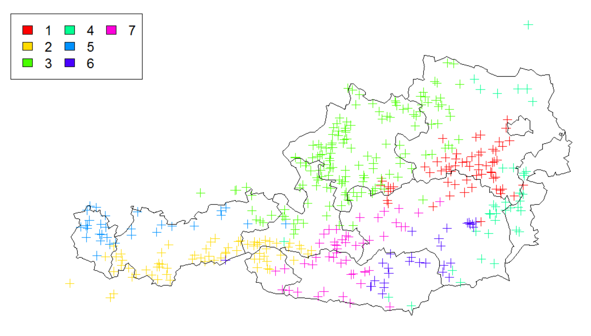
The paper is structured as follows. In Section 2 we provide details on the used data and data preparation. In Section 3 we present the used methodology in detail. We start by giving the rationale of identifying clusters that form the core of the hierarchical dependence structure. Subsequently, we adapt the max-stable processes as suggested in [1] for the dependence modeling of river discharges in river networks to the situation of Austria. This in particular asks for a further branching of hierarchical elements due to the complexity of its topography. We then show how the spatial dependence model that is calibrated on particular measurement stations in the river network can suitably be extended to the level of municipalities. After that, the marginal modeling with both the HORA and the EVA approach is described in detail and compared. Section 4 gives the results for the estimation of the parameters and discusses their implications on the concrete flood risk quantification for all the levels (municipality, state, and country), including the impact on the resulting flood risk diversification potential across these levels. Section 5 then provides some final remarks. Throughout the sections, some technical details as well as the statistical analysis underlying, accompanying, and justifying certain assumptions are delegated to the Appendix A.

2. Data and Normalization

2.1. Damage Data and Normalization

For assessing the magnitude of flood damages, we use the payments of the Austrian catastrophe fund. The fund can compensate private persons for the damage of catastrophic events. We collected the data of the payments for the provinces of Upper Austria (2006–2013), Styria (1989–2013), Lower Austria (2005–2013), and of Salzburg (1991–2013). Data for later years were partially available, but not used here since most of them were not reliable final numbers due to still ongoing settlement procedures. Although the time series of Lower Austria and Upper Austria are relatively short, they at least include the relatively big flood events of 2013 and, for Lower Austria, also 2005. We extracted the data for buildings (including inventory) and for the category “flood” (note, however, that some flood-relevant data points may be missing, as they are possibly stored in the categories “mudflow” (Vermurung) and “landslides” (Hangrutschung), respectively).

To make the damage data usable, we have to normalize them first. In [14] it was shown that the main driver of flood risk change is the change in urban sprawl. To correct for the latter, we correct the data for building stock. The Catastrophe Fund reimburses part of the costs for the rebuilding of the damaged residence buildings, but keeps track of the total costs, an aspect that we use in our analysis. For the normalization, we use the building value of all buildings within a municipality, defined by living space in m² times the construction cost per m². To construct a time series of the building stock in a municipality, we use the data on the living space and living buildings in each municipality (data for the years 1971, 1981, 1991, 2001 were available on a spatial resolution of 5 km (number of flats in different categories) and on 250 m grid (number of buildings). For the period 1966 to 2001 these data were already gathered in the course of the former project [22]. For 2011 we collected the number of residence buildings in each municipality. To get an estimate of the living space in each municipality for 2011, we estimate the average living space per residence building and assume that this quantity stays constant for the time between 2001 and 2011. Between 1971 and 2011 we use cubic spline interpolation to generate the living space and beyond 2011 we extrapolate the function with constant slope, i.e., we assume the relative increase in buildings to be constant (since this concerns only the years 2012 and 2013, this assumption, in any case, has a minor impact on the results). Finally, we normalize the data with the building cost index to account for the aspects of inflation that are relevant to the considered costs.

2.2. Risk Maps

We use the risk maps provided by the HORA system, which provides the flooded areas for floods with return periods of 30, 100, and 200 years, respectively (see [21] for more details). These areas are also called the HQ zones and are available for the entire territory of Austria.

2.3. Discharge Data

For the modeling of the dependence structure, we use river discharges at river gauges and corresponding catchment basins, as well as a river network for Austria. Discharge data for gauges of Austria are obtained from “Hydrographischer Dienst Österreich” [29]. We only use stations with at least 30 years of data, which amounts to 431 stations. Data for the river network and the catchment areas are obtained from Copernicus [30]. Since the resolution of these two datasets does not coincide, we identify each discharge station with the point of the river network that is closest with respect to Euclidean distance. To obtain the basin of a discharge station, we first calculate all river segments upstream of the station and use the associated catchment areas from the Copernicus data set. Furthermore, we remove stations from the dataset that have the same catchment area (i.e., that are on the same river section), after which 425 measurement stations remain for our analysis. With the above-described data, the elevation weighted center of the basin for each discharge station is calculated for later use (as a digital elevation model we use a Digital Elevation Model (DEM) for Austria (at 10 m resolution inside Austria from [31]) and the EU-DEM v1.0 (25 m from Copernicus [32])).

2.4. European Settlement Map

For the distribution of buildings inside each municipality, we use the European Settlement Map (Release 2016) [33].

3. Used Methodology

3.1. Dependence Modeling

We split the modeling of flood risk into two parts. The first part consists of modeling the marginal distribution of flood risk for each municipality. The second part is to use a copula to combine the flood risk of the different municipalities in an appropriate fashion. The choice of copula determines the dependence structure and is hence a crucial step in the modeling. Due to the small number of years with reported damage figures, this is a particular challenge here and cannot reasonably be based on the historical data alone. We, therefore, use the dependence structure inherent in discharge data (for which a much longer and more consistent time series across all of Austria is available) and use it as a proxy for the dependence structure of the flood damages. Such an assumption makes sense, as significant damage can only occur when an extreme discharge is present. At the same time, one has to keep in mind that the link between discharge amounts and flood damage sizes is not deterministic and prone to some inaccuracy. For the dependence structure of discharge levels, we focus on the dependence of extreme discharge only. The latter is the basis for the method proposed in [1], where an analysis for the upper Danube basin is provided. We will mimic this approach but apply it to the entire river network of Austria, for the purpose of which it needs to be extended. This involves the identification of clusters of discharge measurement stations and their combination. Altogether, the dependence modeling will be split into three steps. First, we apply a cluster analysis for regions with similar flood risk. Second, a calibration of the river discharge model will be performed, and finally, the model for measurement stations will be extended to a dependence model among municipalities. We describe these three steps now in more detail.

3.2. Cluster Analysis

A particular motivation to look for clusters comes from [34,35], where regions are defined for the additional consideration of the weather system. Our intention is to find clusters in summer floods, hence we will focus on May to October (cf. [36]). Note that this period is different from the one chosen in [1].

The first step in the cluster analysis is to de-cluster the time series of daily mean discharge. We consider all discharge events that exceed the 90% quantile and apply a 9-day rule, in the sense that events that occur within 9 days are not counted as independent events (such a rule was also used in [1]). This procedure provides us with 848 remaining events, where, in at least one catchment, a peak discharge level above the 90% quantile appeared. Note that an alternative declustering method was used in [37], where two peaks were considered independent if the number of days between them exceeds $4.0483+log \left(A\right)$, where $A$ is the size of the catchment area and the minimal discharge between the peaks is less than three quarters of the smaller discharge of the two peaks. Since in our case the median of the logarithm of the catchment area of the considered measurement stations is $5.1$, our 9-day rule is in fact reasonably in line with that alternative de-clustering method.

We want to cluster measurement stations with respect to the likelihood that extreme discharge levels appear together. As a distance measure, we use the probability that two peaks occur at the same time. We approximate this by the number of common peaks of the 10 largest discharges across the entire period. For the calculation of the clusters, we use hierarchical clustering (the hclust-algorithm in R) with the method ward. D to identify the clusters. This results in 7 clusters in Austria which are depicted in Figure 1. Concretely, this map depicts the altitude-averaged centers of each river basin colored according to the cluster it belongs to. For more details and comments on the clustering, we refer to Appendix A.1.

3.3. The Dependence Model for River Discharge

We need to model extremal dependence in two-dimensional space and for that purpose, max-stable processes (which are an extension of extreme value distributions to the functional setting) have successfully be applied in the extreme value statistics literature (see e.g., [38,39,40]). Whereas the classical approaches were based on assuming that the degree of dependence between two locations depends on the usual Euclidean distance, it was recently proposed in [1] to replace the Euclidean distance by a distance concept that considers flow-connectedness in a river network and the possible exposure to common meteorological events. We will follow that latter approach and adapt it to our setting. In [1] it is assumed that the marginal distribution of the discharge at a point of a river follows a generalized Pareto distribution and that the discharges normalized to unit Fréchet margins follow a (Brown–Resnick) max-stable process defined by

$$\eta \left(t\right)=\underset{i\in \mathbb{N}}{\max }\left(U_i\exp \left(W_i\left(t\right)-\frac{{\sigma }^2\left(t\right)}{2}\right)\right) .$$

Here $t$ represents the location on the river, $U_i$ are the realizations of a Poisson point process with intensity $u^{-2} du,$ and $W_i\left(t\right)$ is a Brownian motion with mean $0$ and variance function ${\sigma }^2\left(t\right)$. It was shown in [41] that the distribution of such a process depends only on the covariance function. For any two locations $s$ and $t$ on the river network, the latter can be defined through a kernel function $\mathsf{\Gamma }\left(s,t\right)$ by

$$\mathbb{E}\left(W^{\left(u\right)}\left(t\right)W^{\left(u\right)}\left(s\right)\right)=\left(\mathsf{\Gamma }\left(s,u\right)+\mathsf{\Gamma }\left(t,u\right)- \mathsf{\Gamma }\left(s,t\right)\right)/2,$$

and

$$\mathbb{E}\left({\left(W^{\left(u\right)}\left(t\right)-W^{\left(u\right)}\left(s\right) \right)}^2 \right)=\mathsf{\Gamma }\left(s,t\right)-\frac{\mathsf{\Gamma }\left(s,s\right)+\mathsf{\Gamma }\left(t,t\right)}{2}=\mathsf{\Gamma }\left(s,t\right).$$

A useful measure for the extremal dependence between two random variables X and Y with distribution functions $F_X$ and $F_Y$ is the so-called extremal coefficient

$$\theta ≔\underset{u\to 1}{\lim }\frac{\mathbb{P}\left(F_X\left(X\right)>u,F_Y\left(Y\right)>u\right)}{1-u},$$

(1)

see for instance [42]. Note that $1\le \theta \le 2,$ where $\theta =1$ corresponds to complete dependence and $\theta =2$ to independence. It has been shown in [41] that

$$\theta \left(s,t\right)=2\mathsf{\Phi }\left(\frac{\sqrt{\mathsf{\Gamma }\left(s,t\right)}}{2}\right),$$

(2)

where $\mathsf{\Phi }\left(x\right)$ is the cumulative distribution function of the standard normal distribution, so that the kernel function $\mathsf{\Gamma }\left(s,t\right)$ directly ‘encodes’ and parametrizes the extremal dependence between two locations $\mathrm{s}$ and $t.$ Small values of $\mathsf{\Gamma }\left(s,t\right)$ correspond to strong dependence and large values correspond to weak dependence. In order to incorporate an appropriate distance concept for the geometry of river discharges, [1] suggested a function $\mathsf{\Gamma }\left(s,t\right)$ of the form

$$\mathsf{\Gamma }\left(\mathrm{s},\mathrm{t}\right)={\lambda }_{Riv}\left\{1-\sqrt{{\pi }_{s,t}} {\left(1-\frac{d\left(s,t\right)}{\tau }\right)}_{+}\right\}+{\lambda }_{Euc}{\left|\left|R\cdot \left(H\left(t\right)-H\left(s\right)\right)\right|\right|}^{\alpha }.$$

The first term in this sum considers hydrological distance in the river network and the second term takes into account dependence resulting from the geographical structure of the river basin and spatially distributed meteorological variables. The two components are combined with weights ${\lambda }_{Riv}$ and ${\lambda }_{Euc}.$The first term is only different from its maximal value 1 if $t$ is downstream of $s$ or $s$is downstream of $t$. Here ${\pi }_{s,t}$is the fraction of the integrated altitude of the catchment basin of the upstream location (which can be seen approximately proportional to the average runoff accumulated in this catchment), divided by the integrated altitude of the (larger) catchment basin of the downstream location. $H\left(t\right)$is the elevation-weighted center of the basin for discharge station $t$, and its use is motivated by the assumption that precipitation is higher for areas with higher elevation, and hence the elevation-weighted center is an approximation for the precipitation-weighted center. The matrix

$$R=\left(\begin{array}{cc}\cos \beta & -\sin \beta \\ c\sin \beta & c\cos \beta \end{array}\right),\frac{\pi }{4}<\beta <\frac{3\pi }{4},c>0$$

takes into account that distance in different directions might not have the same influence on dependence, due to the topography and typical tracks of weather events. For example, if typical events have a track from west to east, then two locations of given distance that lie in east-west direction will be stronger dependent than for a north-west direction. The norm $\left|\left|.\right|\right|$ is the Euclidean norm, and the power $\alpha$ is another constant to be calibrated from the data. Finally, $d\left(s,t\right)$ is the distance of locations $s$ and $t$ along the river network and the constant $\tau >0$ is the maximal distance between two locations until which $\mathsf{\Gamma }\left(\mathrm{s},\mathrm{t}\right)$is influenced by changes in $d\left(s,t\right)$, and is estimated from data. For a more detailed motivation for this particular choice of $\mathsf{\Gamma }\left(\mathrm{s},\mathrm{t}\right)$and further background of its justification we refer to [1] and the references therein.

Whereas [1] only considered the upper catchment area of the Danube, our cluster analysis of the previous section indicates that there might be different processes driving extreme discharge in areas north and south of the Alps. We will, therefore, modify the above process for our purpose to consider the entire region of Austria. Concretely, we will use various distance measures and combine them. The cluster analysis of the previous section is used to group individual stations together into $m$ groups, and we assume that there are $n$ underlying distance kernels ${\mathsf{\Gamma }}_i$-s that lead to extreme discharges. The motivation to use different kernels is that some processes leading to extreme discharge are more local in nature, while others affect a large number of municipalities. Further, we assume that there exist weights ${\lambda }_{i,j} i=1,\dots ,n, j=1,\dots ,m$ such that ${{\displaystyle \sum }}_{i=1}^n{\lambda }_{i,j}^2=1$ and

$$\mathbb{E}\left(W^{\left(u\right)}\left(t\right)W^{\left(u\right)}\left(s\right)\right)={\displaystyle \sum }_{i=1}^n{\lambda }_{i,j\left(s\right)}{\lambda }_{i,j\left(t\right)}\frac{{\mathsf{\Gamma }}_{\mathrm{i}}\left(s,u\right)+{\mathsf{\Gamma }}_{\mathrm{i}}\left(t,u\right)-{\mathsf{\Gamma }}_{\mathrm{i}}\left(s,t\right)}{2},$$

where $j\left(s\right)$ is the cluster to which the location $s$ belongs. Note that when $s$ and $t$ are in the same group, then

$$\mathbb{E}\left({\left(W^{\left(u\right)}\left(t\right)-W^{\left(u\right)}\left(s\right) \right)}^2 \right)={\displaystyle \sum }_{i=1}^n{\lambda }_{i,j\left(s\right)}^2{\mathsf{\Gamma }}_{\mathrm{i}}\left(s,t\right).$$

For the calibration of the resulting dependence model and a discussion and justification for our final choice of $m=7$ and $n=4$, we refer to Appendix A.2.

3.4. The Dependence Model for Municipalities

The approach in the previous subsection provides an approach to model the spatial dependence between individual locations, which we now want to extend to relate the municipalities in Austria. For that, we have to associate the municipalities with river segments. To each municipality, we assign the river segment that is associated to the maximum number of built-up area, using the European Settlement Map in a HQ zone. River distances are then estimated from the end node of a river segment to the start node of another river segment. For the river distance, we additionally assume that if two segments have a common predecessor, then we use the average distance to this common predecessor as the distance between the river segments. This provides us with the river distance between municipalities. The center of the catchment basin associated with a municipality is the weighted average of the center of catchment areas of river segments in the municipality, where the weight is the percentage of built-up area in the HQ-zones associated to the river network. Finally, we assign the municipality to the group for which the mean distance to the next three stations is smallest (distance is between catchment areas).

3.5. Application of the Dependence Model

The resulting dependence model is based on max-stable processes. Since explicit calculations for such processes are not available, we will use Monte-Carlo simulations to generate outcomes and estimate resulting distribution functions and quantiles. The simulation of instances of the underlying max-stable processes is time-consuming; we therefore decide for 100,000 realizations as a reasonable trade-off between accuracy and computation time and power (as we will see later, this leads to confidence intervals for the quantiles of the yearly aggregated damage between 1.5% and 5%, which is quite acceptable). For the calculation of yearly average damage, the error will be higher, but for the latter one can apply the results for independent municipalities (as the average values do not depend on the dependence structure), which is what we will do. Finally, for the simulation of the max-stable process, we use an approximative algorithm, where values below 1/log(2) are not necessarily accurate, but since our focus is the tail, this inaccuracy is not significant for our purposes.

3.6. Risk Map-Based Model

We will improve a model that was used in [21,22]. The HORA system provides the flood areas of floods with return periods of 30, 100 respectively 200 years. These areas are called the HQ zones and are available for the entire territory of Austria. The main idea in [21] was to simulate dependent return periods (which marginally can be seen as realizations of a Pareto random variable with tail parameter 1), and then for each return period in a municipality to estimate the caused damage to the flood with that return period. For that purpose, we first intersect the HQ zones with data on the building stock to get the number of affected buildings in a flood with recurrence level 30, 100, respectively 200 years. For each municipality, these data are then interpolated to get the affected number of buildings for floods with other return periods. Finally, a damage function provides the estimated damage, given the number of affected houses and the return period of the considered flood. These calculations lead to an estimate of the marginal distribution of each municipality. To get an estimate of the distribution of the aggregate (countrywide) damage of a flood event, we then apply in a second step the dependence model described above. We now list some further details on the concrete implementation.

3.7. Interpolation of HQ-Zones

We use the interpolation method of [22]. That is, in the HQ30 zone we use an interpolation according to a beta distribution with parameters $\alpha =4,\beta =1.5$, and in all other HQ zones we use a linear interpolation of buildings (For Vienna, we assume that all buildings are in an ‘artificial’ HQ1000 zone and use linear interpolation to get the number of affected buildings for a flood with smaller return period. Note that the flood risk for Vienna has a very different nature in view of the regulated Danube (and its magnitude is almost negligible when compared to the magnitude of flood risk for the rest of Austria), so that we will include it in this study only in a very limited form).

3.8. Damage Function

The damage of a building is modeled by a lognormal distribution. As in [22,23], we assume that there exists a parameter set for small damages and one for large damages. We model the damage of a building with the small damage distribution (which can be interpreted that only the cellar of the building is affected), unless the flood is unusually large. The latter event is here defined to be one where the flood covers the complete next HQ zone (i.e., a building in the HQ30 zone is hit by a flood with return period larger than 100, or a building in the HQ100 area is hit by a flood with return period larger than 200). In that case, one assumes that the damage is considerably larger since the entire building is damaged, and we then use a different loss distribution.

We use a virtual overbuilt area of 100 m² to characterize a building (note that this value is only important for the number of Lognormal random variables used, and, as discussed in [22], this assumption is not essential for the magnitude of the results). We then approximate the expected damage for each municipality with the available damage data. For that purpose, we first approximate for each municipality the loss degree of damage per overbuilt area by the ratio of the respective maximal yearly damage (in Euro 2015) among the $n$ years of data available in that state and the overbuilt area in the HQ30 zones of that municipality. Note that for $n$ years of damage data, the probability that the maximal damage within these $n$ years is at least as large as a marginal event with a return period of 30 years is given by $q{m}_{30}=1-{\left(1-\frac{1}{30}\right)}^n$. We hence take all these ratios across municipalities in the state and pick the value according to the (empirical) $q{m}_{30}$-quantile, which we assign as an approximation of the expected damage per overbuilt area of a 30-year event. Finally, we take the average of this quantity of all four states for which data are available, and fix this as the expected damage per overbuilt area for small damages across all of Austria. For the final specification of the parameters of the Lognormal distribution, we then choose the variance such that the coefficient of variation is the one for the choice in [21] that was based on further empirical estimates of [16]. Furthermore, we use insight from [16,21] to choose the distribution parameters for the large damages (where the entire building is damaged) by a proportional up-scaling of the distribution for small claims. This entire procedure may be considered somewhat ad-hoc, but is still a rather reasonable approach to use all available damage data as well as insight from other studies to estimate one underlying damage function that is then applied across Austria (one should also keep in mind that in case of many damages, the law of large numbers suggests that finally mainly the expected values matter, which is also observed in the analysis). After normalizing with the estimated damage for 100 m², this eventually leads to the following parameters for the Lognormal distribution of the damage per 100 m²:

$${\mu }_s=2460,{\sigma }_s=1480,{\mu }_l=5676,{\sigma }_l=3517.$$

3.9. Extreme Value Model

While the method of the previous subsection used the claim data only for modeling the average damage per building, not for its entire distribution, we now proceed to an extreme value approach that models the tail directly from the claim data.

A classical result in extreme value theory (see e.g., [43]) states that for a random variable $X$ in the maximum domain of attraction of an extreme value distribution, it holds that

$$li{m}_{u\to \infty }\frac{\mathbb{P}\left(X>u+{\sigma }_{u}s\right)}{\mathbb{P}\left(X>u\right)}={\left(1+\frac{x}{\xi }\right)}^{-\frac{1}{\xi }},$$

where ${\sigma }_u$. is a normalising constant depending on the threshold $u$. This limit motivates the use of a generalized Pareto distribution

$$G_{\xi ,\sigma }\left(x\right)={\left(1+\frac{x}{\xi \sigma }\right)}^{-\frac{1}{\xi }}$$

as a model for the distribution of $X|X>u,$ which we will use on the level of a single municipality. For each municipality $i$ and corresponding claim size random variable $X_i$, we, therefore, assume that there exists a threshold $u_i$ such that the distribution of $X_i|X_i>u_i$ is generalized Pareto with parameter ${\sigma }_i$ and ${\xi }_i$. For simplicity (and analogously to [1]) we assume that the parameter ${\xi }_i$is the same for all municipalities, i.e., ${\xi }_i=\xi \forall i$. Further, we assume that the other parameter ${\sigma }_i$is a linear function of the fraction $\overline{u_i}$of built-up area in the zone HQ100 among the complete built-up area of the municipality and also depends on the state in which the municipality is located. Finally, for the threshold we assume $u_i=\overline{u_i}u$, where $u$ is another fixed quantity, which seems reasonable as the threshold can be higher when there are more buildings at risk.

Given the data and thresholds $u_i$, the estimation of $\xi$ and ${\sigma }_i$ is a standard procedure (cf. [44]), and we will use the function gpd.fit from the R-package ismev. For the estimation of $u_i$ there exists no standard method. We split the task of estimating $u_i$ into two subtasks. First, we will estimate the $\overline{u_i}$ from the damage data and then use a Hill-type plot for different values of $u$. To get a complete model for the $X_i$, we finally need the probability $\mathbb{P}\left(X_i>u_i\right)$ of having a claim larger than the threshold, which we estimate using the data of Salzburg and Styria only (since the time series for Upper and Lower-Austria are too short for this purpose) and the distribution of $X_i|X_i\le u_i$, for which we simply use the empirical distribution. We refer to Appendix A.3 for further details.

4. Main Results

In the previous section, we have developed two (statistical) models for the assessment of flood risks in Austrian municipalities. The first (HORA) model can be applied to all municipalities in Austria. The applications of the second (EVA) model is restricted to municipalities where claim data exist. We then use Monte Carlo simulations to obtain estimates for the average yearly damages and the quantiles. On the marginal distribution level, the differences between the two approaches are discussed and analyzed in detail in Appendix A.4. We will then apply our dependence model, and also complement the final results by respective estimates under the assumption that flood risk of the municipalities is independent (no dependence) and that it is comonotone (complete dependence cf. [45]). This allows to illustrate best- and worst-case bounds concerning the sensitivity of the results with respect to the implemented dependence structure. The comparison with extreme dependence scenarios is also helpful to assess the presence of diversification potential of flood risk.

4.1. Results for Austria

In

Table 1. Average yearly damage and estimated damage (in mio. €) for floods with return periods of 30, 100, 200, and 300 years for Austria (based on the HORA model with the estimated dependence structure, and in comparison with the case of independence and comonotone dependence). Numbers in parentheses are the 95% confidence intervals from the Monte Carlo simulation (For the calculation of a two-sided distribution-free (slightly conservative) confidence interval for a quantile $q,$ we use the formula ${\widehat{F}}^{-1}\left(q\pm z_{1-\alpha } \sqrt{\frac{q\left(1-q\right)}{n}}\right),$ where $z_{1-\alpha }$ is the $\left(1-\alpha \right)$-quantile of the standard normal distribution and ${\widehat{F}}^{-1}$ is the inverse of the empirical distribution function, cf. [47] for a motivation of this formula, where we approximate the binomial distribution by a normal distribution. Note that the resulting confidence interval is not necessarily symmetric around the estimate).

	Average	30	100	200	300
Model	80.8	515	1250	1880	2300
	(78.6–83.1)	(501–531)	(1200–1290)	(1800–1990)	(2190–2410)
Independent	84.2	157	197	224	245
	(84–84.4)	(156–158)	(194–199)	(221–227)	(239–254)
Comonotone	86.7	1080	2600	3050	3360
	(82.8–90.6)	(1060–1080)	(1270–2610)	(2760–3110)	(3280–3450)
Ratio Com/Model		48%	48%	62%	68%

we present the average yearly damage as well as the expected damage for a flood event with return period of 30, 100, 200, and 300 years for Austria as obtained by the HORA model. Note that the expected damage of a flood with a return period of 200 years is particularly interesting in terms of risk management (since the 200-year value at risk is the relevant quantity for the required safety capital for insurance in the European Union). For the average yearly damage, we get values between 80.8 mio. € and 86.7 mio. €. Theoretically, all models should provide the same average value, but the Monte Carlo estimate naturally has some variance. Since this latter variance will be larger when spatial dependence is involved, we favor here the estimate based on independent flood risk between municipalities and will, therefore, use the corresponding result of 84.2 mio. € for the yearly average damage as the benchmark for the later comparisons.

A flood with a return period of 200 years has an expected damage of about 1.9 billion €, which is approximately 22 times the average yearly damage. In other words, one has to save the average yearly damage of 22 years as solvency capital for a 200-year flood event. Comparing the results for the estimated dependence structure with the one for independence and comonotone dependence, we see that the estimated quantiles are much closer to the comonotone case, illustrating and quantifying the strong spatial dependence for flood risk in Austria. Note that for given marginal distributions for each municipality, under comonotonicity, the quantile for the aggregate risk is the sum of the individual quantiles, see e.g., [46]. In other words, since the quantile of the loss distribution is linked to the solvency capital requirement for a flood insurance activity, the respective figures in the third row of Table 1 can be interpreted as the overall amount of needed (stand-alone) solvency capital, if all municipalities would insure their flood risk on their own, whereas the figures in the first row reflect the respective capital requirement when the flood risk is pooled on the aggregate Austrian level. The ratio in the last row is hence an indication for the diversification potential in flood risk (e.g., for the relevant 200-year return level, one can reduce the amount of required solvency capital by pooling all flood risk in Austria by 38%). At the same time, given the many individual municipalities involved, this also reflects the strong spatial dependence present in flood risk, as one a priori may expect a larger reduction on the aggregate level.

4.2. Results for the States of Austria

In

Table 2. Average yearly damage and estimated damage (in mio. €) for floods with return periods of 30 and 200 years, for the states of Austria. The damage is calculated with the HORA model and with three different dependence structures between the municipalities (the estimated dependence structure of this paper, independence and comonotone dependence). Numbers in parentheses are the 95% confidence intervals from the Monte Carlo simulation.

	B	K	NÖ	OÖ	ST	S	T	V
Average (Independent)	3.29	6.39	22.8	15.5	11.5	7.14	11.6	5.68
	(3.27–3.31)	(6.32–6.45)	(22.8–22.9)	(15.4–15.6)	(11.4–11.6)	(7.06–7.22)	(11.5–11.7)	(5.63–5.74)
Average (Comonotone)	3.42	6.59	23.5	16	11.9	7.29	11.9	5.79
	(3.22–3.61)	(6.31–6.87)	(22.5–24.6)	(15.2–16.8)	(11.3–12.6)	(7.01–7.58)	(11.4–12.3)	(5.6–5.98)
Average (Model)	3.23	6.1	22.2	14.6	11	6.81	11.2	5.49
	(3.08–3.37)	(5.92–6.28)	(21.5–22.9)	(14.1–15.2)	(10.6–11.4)	(6.59–7.03)	(10.8–11.5)	(5.33–5.65)
30 (Model)	22.7	46.5	158	111	76.1	56.8	88.4	52.6
	(21.9–23.6)	(45.5–47.7)	(154–163)	(107–115)	(73.7–78.9)	(54.9–58.8)	(86.2–91.2)	(50.6–54.8)
30 (Independent)	9.51	23.4	56.8	42.5	30.9	33	47.3	24.7
	(9.4–9.66)	(23–23.8)	(56.1–57.5)	(42–43)	(30.6–31.3)	(32.8–33.2)	(46.8–47.7)	(24.5–25)
30 (Comonotone)	39.3	85.1	283	194	140	95.4	158	81.6
	(38.6–39.5)	(83.5–85.4)	(277–285)	(190–195)	(137–141)	(93.5–95.9)	(155–159)	(80.1–82)
Ratio 30 Com/Model	58%	55%	56%	57%	54%	60%	56%	64%
200 (Model)	87.9	159	642	443	295	206	309	179
	(84.5–92)	(152–165)	(610–674)	(427–462)	(282–309)	(198–215)	(295–318)	(174–185)
200 (Independent)	20.1	52.5	84.6	87	72.8	80.9	111	52.9
	(19.5–20.7)	(51.4–53.6)	(83.4–85.9)	(85–89.3)	(70.8–74.4)	(79.7–81.8)	(110–112)	(52.3–53.4)
200 (Comonotone)	109	222	899	537	399	256	422	206
	(98.8–112)	(206–227)	(796–914)	(486–551)	(356–409)	(235–260)	(387–428)	(194–208)
Ratio 200 Com/Model	81%	72%	71%	82%	74%	80%	73%	87%

, we break down the results to the level of individual states in Austria. We again present the average yearly damage as well as the expected damage for a flood event with return period of (for brevity now only) 30 and 200 years for all states of Austria as obtained by the HORA model (While we did include Vienna for the results of the entire country of Austria for completeness, as mentioned before we do not provide a detailed separate analysis on its state level due to its very different characteristic in view of river regulations. Note that its average yearly damage measured akin to the other states in Table 2 would amount to 0.24, the estimated damage for a return period of 30 years is virtually 0 and for a return period of 200 an analogous estimate would be 4.35 mio. €, clearly indicating that flood risk for Vienna is negligible on the Austrian scale). We provide the results again for the three used dependence structures (independence, comonotone and the estimated dependence structure). We see from the ratios that the diversification potential within each state is now only around 20% for the 200-year event quantile levels (which can be translated into possible solvency capital reduction) compared to stand-alone management of each municipality. It was to be expected that this amount is reduced relative to pooling across all of Austria (since spatial dependence within each state is naturally stronger than across the entire country). However, the concrete numbers nicely allow to quantify how much one gains—on average—by pooling flood risk across the entire country (note that the financial management of flood risk in Austria is to quite some extent politically a competence of each state separately, so that policy recommendations towards collaboration may originate from the present considerations). Concretely, summing the 200-year return period quantiles of all the individual states (here even including the small value for Vienna), we arrive at an over-all potential solvency capital requirement of 2.32 bio. €, which can be compared with the 1.88 bio. € obtained for the entire country of Austria above. That is, pooling the risk of the states on the Austrian level leads to a solvency capital reduction of about 500 mio. €, when measured in these terms. Comparing these results further with the ones of independent risks, we may still conclude that the diversification effect for flood risk is altogether relatively small, and that flood risk in Austria is quite concentrated. When comparing to the respective damage figures of the 30-year return period, one observes that this concentration is considerably stronger in the tail (i.e., for higher quantiles).

4.3. Results for Municipalities with Claim Data

For those municipalities where claim data from the past are available, we can now also apply our second (EVA) model, which provides a sort of local refinement. In the present study, we could use data for municipalities in Lower and Upper Austria, Styria and Salzburg. Before we proceed to the presentation of the results, let us consider some empirical statistics for these data (which are normalized with respect to the building cost index) in

Table 3. Empirical statistics for the normalized damage data for the states with data. Maximal, minimal, average, and median yearly damage (in mio. €) and the number of years with available data. Numbers in parenthesis are the 95% confidence intervals from the Monte Carlo Simulation.

	Max	Average	Median	Min	# Years
ST	32.2	5.2	1.78	0.066	25
OÖ	86.9	12.3	1.59	0.302	8
NÖ	77.8	28.0	9.04	1.9	9
S	52.6	4.0	0.18	0.009	23

.

For purposes of comparison, we first present in

Table 4. Average yearly damage and estimated damage (in mio. €) for floods with return periods of 30, 100, 200, and 300 years, for the municipalities with claim data. The damage is calculated with the HORA model and with three different dependence structures between the municipalities (the estimated dependence structure of this paper, independence, and comonotone dependence). Numbers in parentheses are the 95% confidence intervals from the Monte Carlo simulation.

	Average	30	100	200	300
Model	51.1	343	878	1300	1630
	(49.5–52.7)	(334–353)	(846–918)	(1270–1370)	(1540–1740)
Independent	53.1	103	133	154	170
	(52.9–53.3)	(102–104)	(130–134)	(151–157)	(163–175)
Comonotone	54.9	658	1600	1940	2170
	(52.3–57.5)	(643–660)	(794–1620)	(1740–1990)	(2110–2230)

the respective results of the HORA Model for the aggregation of all the municipalities with available claim data. From the average loss amounts in that table one deduces that more than 60% of the flood risk (in terms of expected claim amounts) in Austria is in fact concentrated in those municipalities.

When comparing the results of the HORA model with the empirical claim statistics in Table 3, one can sum the empirical averages of the annual claims of the four states, which in fact quite well corresponds to the model average in Table 4 (note that for the latter the historical claim sizes were only used in a very peripheral way when estimating the mean damage of individual buildings!). Also, given the almost 30 years of claim experience for Styria and Salzburg, one could interpret that the maximal claim amount over the available years is a reasonable approximation to the 30-year quantile (although with a considerable uncertainty). For Upper and Lower Austria, less than 10 years of data are available, but there we know that we have one (Upper Austria) and two (Lower Austria) historically big flood events in the data, so that the maximum there may also be an indicator towards the 30-year quantile. Despite the hand-waving nature of this interpretation, one sees that indeed the magnitude of the 30-year quantiles of the model are in a reasonable range when compared to the empirical data.

Table 5. Average yearly damage and estimated damage (in mio. €) for floods with return periods of 30, 100, 200, and 300 years, for the municipalities with claim data. The damage is calculated with the Extreme Value Analysis (EVA) model and with three different dependence structures between the municipalities (the estimated dependence structure of this paper, independence and comonotone dependence). Numbers in parenthesis are the 95% confidence intervals from the Monte Carlo Simulation.

	Average	30	100	200	300
Model	65.3	178	683	1440	2000
	(44.1–86.5)	(169–187)	(633–748)	(1270–1630)	(1830–2300)
Independent	68.2	205	510	868	1210
	(64.7–71.6)	(200–210)	(487–531)	(812–937)	(1130–1360)
Comonotone	49.5	49.1	776	1580	2330
	(43–56)	(48.5–159)	(732–831)	(1450–1710)	(2130–2540)

now presents the respective results for the EVA Model for the same municipalities. One sees that the estimated average annual damage is about 30% larger for the EVA model than for the HORA model. Looking at the resulting numbers for different return periods, we see that the EVA model gives considerable more weight to the tail of the distribution (which may be most easily visible when considering the numbers under the independence assumption). Yet, except for the 30- year quantile, the quantiles of the two models are relatively close (especially when one compares the ratio of the quantiles over the mean (16.5 vs. 10 times the mean for the 100 year-quantile, 24.4 vs. 21.1 times the mean for the 200-year quantile, 30.7 vs. 29.3 times the mean for the 300 year-quantile). Nevertheless, in absolute numbers the increase in expected damage as function of the return period is considerably bigger for the EVA method.

5. Discussion and Conclusions

In this paper, we made two main contributions to the flood risk literature. Firstly, we introduced a new approach to model the dependence structure that can be used to aggregate the information of existing risk maps to larger areas. Concretely, we suggested a spatial dependence structure that is calibrated with publicly available data of river discharges and the river network. Hence it is easily applicable to any region in Europe without the need of a hydrological model. The second contribution is to use historical claim data of municipalities for the estimation of future flood risks to obtain an alternative estimate which can either be used directly or as a benchmark for other approaches. We exemplified our approach for the country of Austria.

The choice of a dependence structure is a crucial step when aggregating individually modeled risks onto a collective level. For flood risk applications, a reliable dependence structure allows to aggregate the risk of flood damages from individual municipalities to bigger areas like states or the entire country. The resulting aggregate distribution can then be used to estimate important quantities for risk management like the required solvency capital (e.g., the expected damage of a flood with return period of 200 years in the regulatory framework of the European Union). Comparing the required solvency capital for a calibrated dependence structure with the corresponding numbers for comonotone risks subsequently quantifies diversification effects in the process of flood damage aggregation. In this paper, we developed a concrete and detailed case study for Austria. We first used the HORA risk map available in Austria and intertwined it with the building structure at a fine resolution. We then estimated loss distributions for each municipality in Austria for any flood event with a given return period. The obtained marginal flood damage distributions per municipality were then combined with a spatial dependence model based on a max-stable process to obtain the distribution of flood risks on various levels of aggregation. Here the dependence model was calibrated using the joint occurrences of river discharge levels in the Austrian river network. Monte Carlo simulations of joint appearances of return periods were then implemented to obtain flood loss distributions for each municipality and its aggregations.

The resulting model leads to a projected reduction of required solvency capital for the individual states of Austria between 29% for Lower Austria and 13% for Vorarlberg when compared to assuming the risks separately on the individual municipality levels. One also obtains that the states of Salzburg, Upper Austria, Vorarlberg and Burgenland have a higher concentrated risk than the other states. We have also seen that a further aggregation onto the country level is definitely worthwhile and leads to an overall reduction of required solvency capital of about 38% when compared to the sum of capital requirements of all individual municipalities. We additionally compare the results with the ones under an independence and a comonotone dependence assumption between municipalities, which reveals that the actual situation is much closer to comonotonic dependence than to independence, indicating that flood risk in Austria is particularly difficult to diversify and needs a substantial amount of scrutiny in its management.

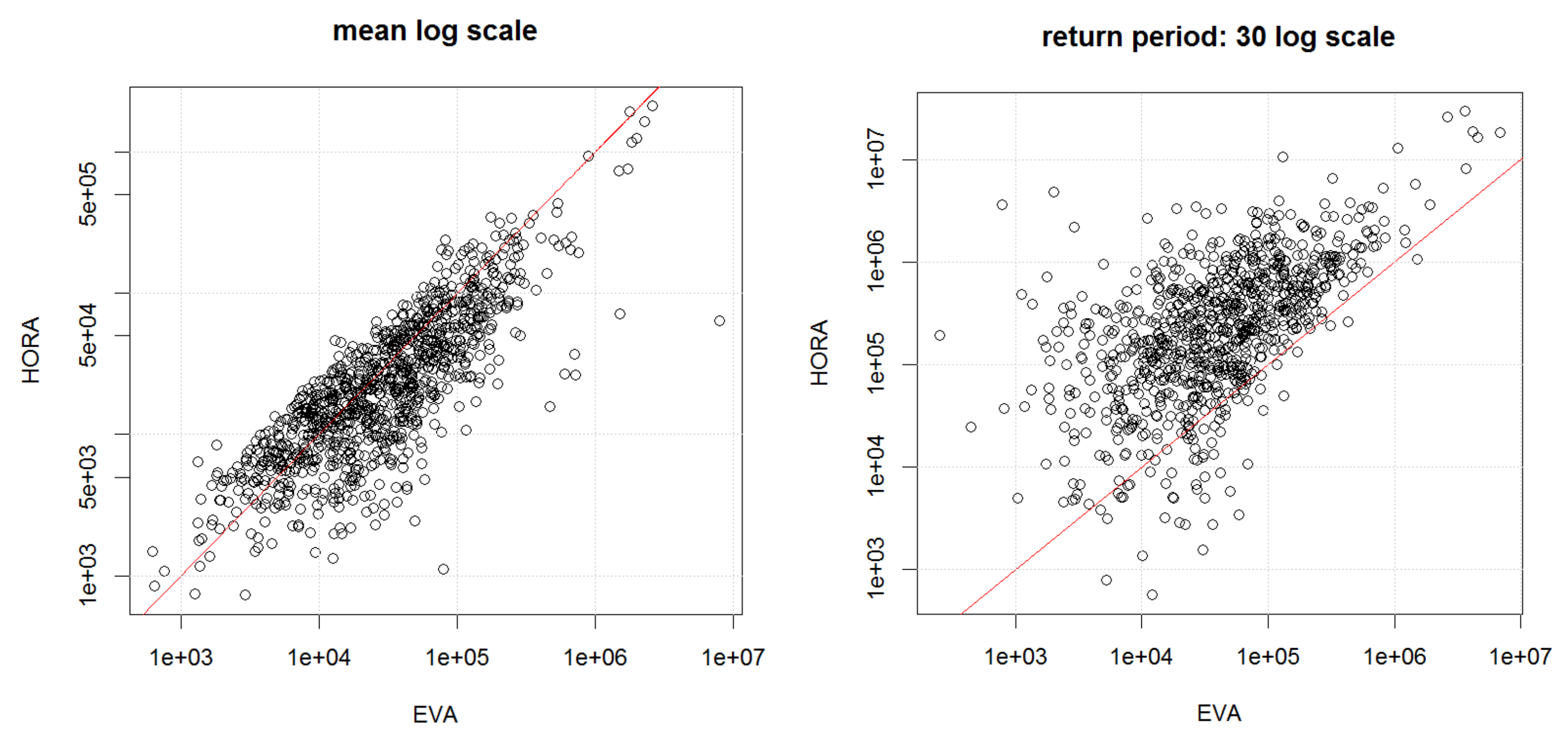
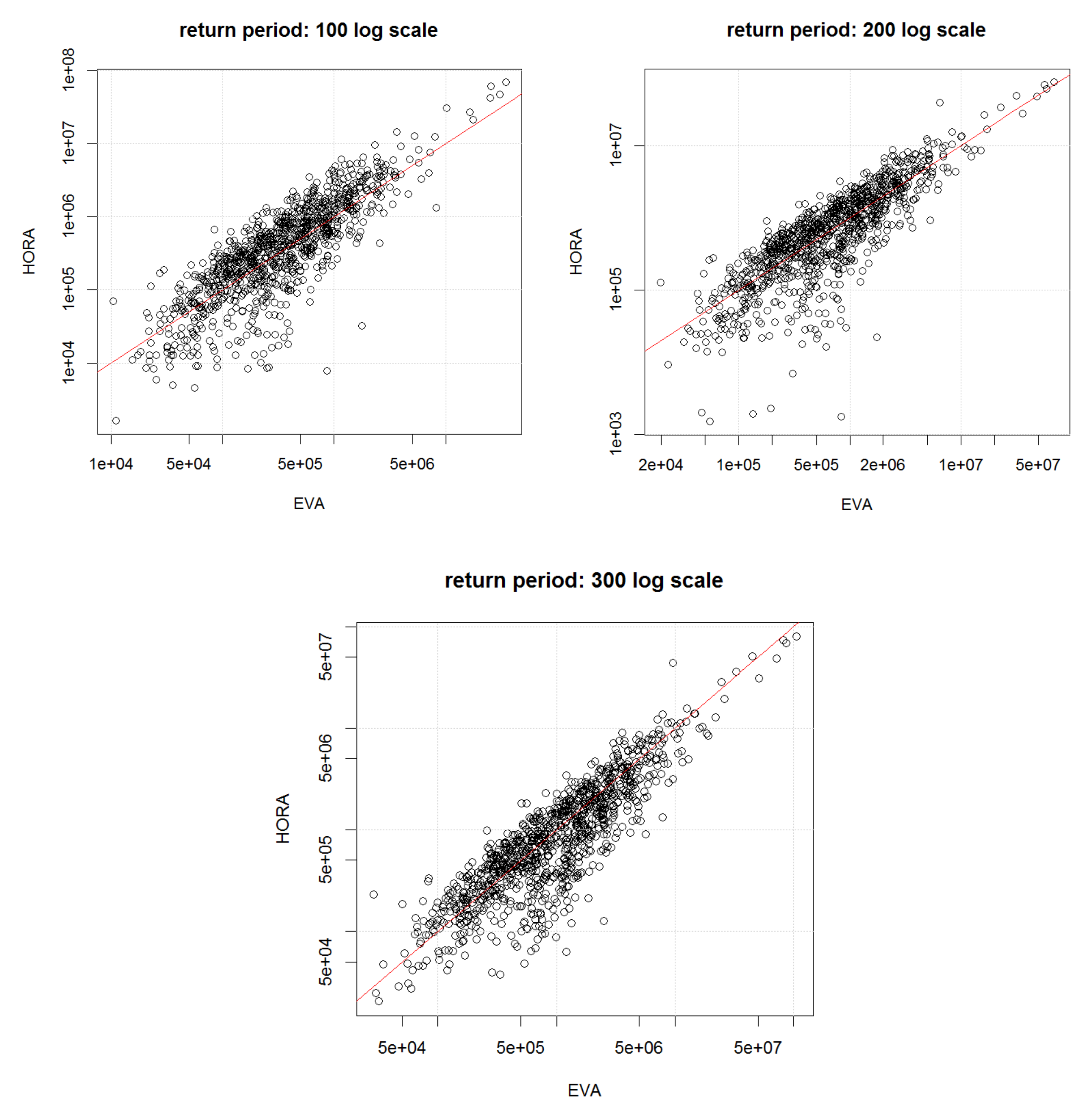
As a complement to the HORA model, we also developed a model based on real historical claim data for Austria and an extreme value analysis (EVA) approach to fit the suitably normalized flood losses for each municipality. Firstly, the actual claim data allowed to challenge the findings of the HORA model as the latter is not based on historical data, suggesting consistency for three of the four states with claim data (although this comparison between the actual claims and the HORA estimates should not be over-emphasized given the limited amount of years with available claim data).

Combining the obtained marginal distributions in the EVA approach again with the same spatial dependence model as for the HORA method then led to an alternative approach to quantify aggregate flood risk on a state and country level. Compared to the earlier study [21] of flood risk in Austria, the present contribution not only uses a considerably improved dependence model, but also much more refined data for the marginal behavior, so that we were able to sharpen those previous results considerably. The new estimates suggest a reduction of the projected flood damage based on historical claim data compared to the earlier study. In comparison to the HORA model, the EVA approach leads to higher expected annual damages and more mass in the tail of the distribution. Nevertheless, in the range of flood damages for a return period of 200 years, a quantity that is relevant for risk management purposes related to Solvency 2 in the European Union, the results for the HORA and the EVA model are quite similar. This is remarkable, as the two approaches use empirical data and relations in quite a different way, indicating some robustness of the obtained magnitudes.

As mentioned in the introduction, the dependence modeling approach proposed in this paper can be applied to any other country, if marginal modeling experience and river discharge information is available, and it could be nice to see how the respective estimates for average and extreme flood losses compare to findings of other studies, often relying on hydrological models. While the present study took the non-stationarity of flood risk into account in terms of inflation correction, changes in building structure over time, and adaptations to the risk maps, it will be interesting in future research to also combine this approach with longer-term experience and projections due to climate risk. This could for instance include the consideration of time-dependent parameters in the max-stable components based on longer-term experience of flood occurrences (see e.g., [48]) or even paleo-floods (see e.g., [49]). Also, one might lift the granular dependence model approach suggested in this paper up one more level to the entire river network of Europe and in that way refine the somewhat coarse Clayton copula approach underlying the interesting findings in [4].

We would like to finish with some remarks on uncertainties. While one can quantify the error that comes from the numerical evaluation of the quantiles by Monte Carlo estimation from the specified model (and we have done so in the respective tables), the model choice itself naturally is another source of uncertainty for final estimates that cannot be quantified in a straight-forward way, and is, in fact, present in any modeling approach. Uncertainties of the HORA model are already discussed in [21], and mainly are the number of buildings affected by a flood for a given return period, the average damage of a building in a flood with a given return period and the used dependence structure for aggregating the risk of individual municipalities. Among these, the number of buildings affected by a flood of a given return period is probably the major source of uncertainty about the results, but since this error depends on the geographic characteristics of the municipality, it is hard to quantify with statistical methods. However, in this paper, the HORA model was complemented by a second, different approach using EVA techniques. The latter has considerable uncertainties itself, which mainly stem from the extrapolation nature of the method, but the comparison of the two different methods in fact assesses to some extent model risk in the calculations. Finally, adding the scenarios with comonotone and with independent risks in the analysis of this paper enabled us to establish best- and worst-case bounds for our results concerning the underlying dependence assumptions. In particular, the respective numbers can help to decide, in future studies, whether to focus more particularly on these aspects of the modeling procedure.

References

1. Asadi, P.; Davison, A.C.; Engelke, S. Extremes on river networks. Ann. Appl. Stat. 2015, 9, 2023–2050. [Google Scholar] [CrossRef]
2. Alfieri, L.; Bisselink, B.; Dottori, F.; Naumann, G.; de Roo, A.; Salamon, P.; Wyser, K.; Feyen, L. Global projections of river flood risk in a warmer world: River flood risk in a warmer world. Earths Future 2017, 5, 171–182. [Google Scholar] [CrossRef]
3. Winsemius, H.C.; Aerts, J.C.J.H.; van Beek, L.P.H.; Bierkens, M.F.P.; Bouwman, A.; Jongman, B.; Kwadijk, J.C.J.; Ligtvoet, W.; Lucas, P.L.; van Vuuren, D.P.; et al. Global drivers of future river flood risk. Nat. Clim. Chang. 2016, 6, 381–385. [Google Scholar] [CrossRef]
4. Jongman, B.; Hochrainer-Stigler, S.; Feyen, L.; Aerts, J.C.J.H.; Mechler, R.; Botzen, W.J.W.; Bouwer, L.M.; Pflug, G.; Rojas, R.; Ward, P.J. Increasing stress on disaster-risk finance due to large floods. Nat. Clim. Chang. 2014, 4, 264–268. [Google Scholar] [CrossRef]
5. Dottori, F.; Salamon, P.; Bianchi, A.; Alfieri, L.; Hirpa, F.A.; Feyen, L. Development and evaluation of a framework for global flood hazard mapping. Adv. Water Resour. 2016, 94, 87–102. [Google Scholar] [CrossRef]
6. Dottori, F.; Szewczyk, W.; Ciscar, J.-C.; Zhao, F.; Alfieri, L.; Hirabayashi, Y.; Bianchi, A.; Mongelli, I.; Frieler, K.; Betts, R.A.; et al. Increased human and economic losses from river flooding with anthropogenic warming. Nat. Clim. Chang. 2018, 8, 781. [Google Scholar] [CrossRef]
7. Willner, S.N.; Otto, C.; Levermann, A. Global economic response to river floods. Nat. Clim. Chang. 2018, 8, 594. [Google Scholar] [CrossRef]
8. Falter, D.; Schröter, K.; Dung, N.V.; Vorogushyn, S.; Kreibich, H.; Hundecha, Y.; Apel, H.; Merz, B. Spatially coherent flood risk assessment based on long-term continuous simulation with a coupled model chain. J. Hydrol. 2015, 524, 182–193. [Google Scholar] [CrossRef]
9. Falter, D.; Dung, N.V.; Vorogushyn, S.; Schröter, K.; Hundecha, Y.; Kreibich, H.; Apel, H.; Theisselmann, F.; Merz, B. Continuous, large-scale simulation model for flood risk assessments: Proof-of-concept. J. Flood Risk Manag. 2016, 9, 3–21. [Google Scholar] [CrossRef]
10. Willner, S.N.; Levermann, A.; Zhao, F.; Frieler, K. Adaptation required to preserve future high-end river flood risk at present levels. Sci. Adv. 2018, 4, eaao1914. [Google Scholar] [CrossRef] [Green Version]
11. Mechler, R.; Bouwer, L.M.; Linnerooth-Bayer, J.; Hochrainer-Stigler, S.; Aerts, J.C.J.H.; Surminski, S.; Williges, K. Managing unnatural disaster risk from climate extremes. Nat. Clim. Chang. 2014, 4, 235–237. [Google Scholar] [CrossRef]
12. Prettenthaler, F.; Amrusch, P.; Habsburg-Lothringen, C. Estimation of an absolute flood damage curve based on an Austrian case study under a dam breach scenario. Nat. Hazards Earth Syst. Sci. 2010, 10, 881–894. [Google Scholar] [CrossRef]
13. Elmer, F.; Thieken, A.H.; Pech, I.; Kreibich, H. Influence of flood frequency on residential building losses. Nat. Hazards Earth Syst. Sci. 2010, 10, 2145–2159. [Google Scholar] [CrossRef] [Green Version]
14. Elmer, F.; Hoymann, J.; Düthmann, D.; Vorogushyn, S.; Kreibich, H. Drivers of flood risk change in residential areas. Nat. Hazards Earth Syst. Sci. 2012, 12, 1641–1657. [Google Scholar] [CrossRef] [Green Version]
15. Merz, B.; Kreibich, H.; Lall, U. Multi-variate flood damage assessment: A tree-based data-mining approach. Nat. Hazards Earth Syst. Sci. 2013, 13, 53–64. [Google Scholar] [CrossRef]
16. Merz, B.; Kreibich, H.; Thieken, A.; Schmidtke, R. Estimation uncertainty of direct monetary flood damage to buildings. Nat. Hazards Earth Syst. Sci. 2004, 4, 153–163. [Google Scholar] [CrossRef] [Green Version]
17. Wagenaar, D.J.; de Bruijn, K.M.; Bouwer, L.M.; de Moel, H. Uncertainty in flood damage estimates and its potential effect on investment decisions. Nat. Hazards Earth Syst. Sci. 2016, 16, 1–14. [Google Scholar] [CrossRef] [Green Version]
18. Merz, R.; Blöschl, G.; Humer, G. National flood discharge mapping in Austria. Nat. Hazards 2008, 46, 53–72. [Google Scholar] [CrossRef]
19. Vorogushyn, S.; Bates, P.D.; de Bruijn, K.; Castellarin, A.; Kreibich, H.; Priest, S.; Schröter, K.; Bagli, S.; Blöschl, G.; Domeneghetti, A.; et al. Evolutionary leap in large-scale flood risk assessment needed. Wiley Interdiscip. Rev. Water 2018, 5, e1266. [Google Scholar] [CrossRef] [Green Version]
20. McNeil, A.J.; Frey, R.; Embrechts, P. Quantitative Risk Management: Concepts, Techniques and Tools-Revised Edition; Princeton University Press: Princeton, NJ, USA, 2015. [Google Scholar]
21. Prettenthaler, F.; Kortschak, D.; Hochrainer-Stigler, S.; Mechler, R.; Urban, H.; Steininger, K.W. Catastrophe management: Riverine flooding. In Economic Evaluation of Climate Change Impacts: Development of a Cross-Sectoral Framework and Results for Austria; Steininger, K.W., König, M., Bednar-Friedl, B., Kranzl, L., Loibl, W., Prettenthaler, F., Eds.; Springer Climate; Springer International Publishing: Cham, The Netherlands, 2015; pp. 349–366. ISBN 978-3-319-12457-5. [Google Scholar]
22. Hochwasser und dessen Versicherung in Österreich; Albrecher, H.; Prettenthaler, F. (Eds.) Verlag der Österreichischen Akademie der Wissenschaften: Wien, Austria, 2009; Volume III, ISBN 978-3-7001-6753-2. [Google Scholar]
23. Url, T. Wahrscheinlichkeits-Überschreitungskurven für Hochwasserkatastrophen in Österreich; WIFO-Österreichisches Institut für Wirtschaftsforschung: Wien, Austria, 2008. [Google Scholar]
24. Barendrecht, M.H.; Viglione, A.; Kreibich, H.; Vorogushyn, S.; Merz, B.; Blöschl, G. Estimating parameter values of a socio-hydrological flood model. In Proceedings of the International Association of Hydrological Sciences; Copernicus GmbH; IAHS: Wallingford, UK, 2018; Volume 379, pp. 193–198. [Google Scholar]
25. Aerts, J.C.J.H.; Botzen, W.J.; Clarke, K.C.; Cutter, S.L.; Hall, J.W.; Merz, B.; Michel-Kerjan, E.; Mysiak, J.; Surminski, S.; Kunreuther, H. Integrating human behaviour dynamics into flood disaster risk assessment. Nat. Clim. Chang. 2018, 8, 193. [Google Scholar] [CrossRef] [Green Version]
26. Barendrecht, M.H.; Viglione, A.; Kreibich, H.; Merz, B.; Vorogushyn, S.; Blöschl, G. The value of empirical data for estimating the parameters of a sociohydrological flood risk model. Water Resour. Res. 2019, 55, 1312–1336. [Google Scholar] [CrossRef] [PubMed] [Green Version]
27. Prettenthaler, F.; Albrecher, H.; Köberl, J.; Kortschak, D. Risk and insurability of storm damages to residential buildings in Austria. Geneva Pap. Risk Insur. Issues Pract. 2012, 37, 340–364. [Google Scholar] [CrossRef]
28. Prettenthaler, F.; Albrecher, H. (Eds.) Sturmschäden: Modellierung der versicherten Schäden in Österreich; Verlag der Österreichischen Akademie der Wissenschaften: Wien, Austria, 2012. [Google Scholar]
29. eHYD—der Zugang zu Hydrographischen Daten Österreichs. Available online: https://ehyd.gv.at/ (accessed on 10 September 2019).
30. EU-Hydro—Copernicus Land Monitoring Service. Available online: https://land.copernicus.eu/imagery-in-situ/eu-hydro (accessed on 10 September 2019).
31. Digitales Geländemodell (DGM) Österreich—data.gv.at. Available online: https://www.data.gv.at/katalog/dataset/b5de6975-417b-4320-afdb-eb2a9e2a1dbf (accessed on 10 September 2019).
32. EU-DEM v1.0—Copernicus Land Monitoring Service. Available online: https://land.copernicus.eu/imagery-in-situ/eu-dem/eu-dem-v1-0-and-derived-products/eu-dem-v1.0 (accessed on 10 September 2019).
33. European Settlement Map—Copernicus Land Monitoring Service. Available online: https://land.copernicus.eu/pan-european/GHSL/european-settlement-map (accessed on 10 September 2019).
34. Merz, R.; Blöschl, G. Process controls on the statistical flood moments—A data based analysis. Hydrol. Process. 2009, 23, 675–696. [Google Scholar] [CrossRef]
35. Hofstätter, M.; Beck, C.; Chimani, B.; Ganekind, M.; Homan, M.; Jacobeit, J.; Phillip, A. WETRAX: WEather Patterns, Cyclone TRAcks and related precipitation EXtremes. In Proceedings of the European Geosciences Union General Assembly 2013, Vienna, Austria, 7–12 April 2013; Volume 15. EGU2013–5145. [Google Scholar]
36. Blöschl, G.; Viglione, A.; Merz, R.; Parajka, J.; Salinas, J.L.; Schöner, W. Auswirkungen des klimawandels auf hochwasser und niederwasser. Österr. Wasser Abfallw. 2011, 63, 21–30. [Google Scholar] [CrossRef]
37. Mediero, L.; Kjeldsen, T.R.; Macdonald, N.; Kohnova, S.; Merz, B.; Vorogushyn, S.; Wilson, D.; Alburquerque, T.; Blöschl, G.; Bogdanowicz, E.; et al. Identification of coherent flood regions across Europe by using the longest streamflow records. J. Hydrol. 2015, 528, 341–360. [Google Scholar] [CrossRef] [Green Version]
38. Opitz, T. Extremal t processes: Elliptical domain of attraction and a spectral representation. J. Multivar. Anal. 2013, 122, 409–413. [Google Scholar] [CrossRef]
39. Schlather, M. Models for stationary max-stable random fields. Extremes 2002, 5, 33–44. [Google Scholar] [CrossRef]
40. Brown, B.M.; Resnick, S.I. Extreme values of independent stochastic processes. J. Appl. Probab. 1977, 14, 732–739. [Google Scholar] [CrossRef]
41. Kabluchko, Z. Extremes of independent gaussian processes. Extremes 2011, 14, 285–310. [Google Scholar] [CrossRef] [Green Version]
42. Ledford, A.W.; Tawn, J.A. Statistics for near independence in multivariate extreme values. Biometrika 1996, 83, 169–187. [Google Scholar] [CrossRef] [Green Version]
43. Beirlant, J.; Goegebeur, Y.; Segers, J.; Teugels, J.L. Statistics of Extremes: Theory and Applications; John Wiley & Sons: Hoboken, NJ, USA, 2004. [Google Scholar]
44. Coles, S. An Introduction to Statistical Modeling of Extreme Values; Springer Series in Statistics; Springer: London, UK, 2001; ISBN 978-1-85233-459-8. [Google Scholar]
45. Nelsen, R.B. An Introduction to Copulas; Springer Science & Business Media: Berlin/Heidelberg, Germany, 2007. [Google Scholar]
46. Dhaene, J.; Vanduffel, S.; Tang, Q.; Goovaerts, M.J.; Kaas, R.; Vyncke, D. Capital requirements, risk measures and comonotonicity. Belg. Actuar. Bull. 2004, 4, 53–61. [Google Scholar]
47. Hahn, G.J.; Meeker, W.Q. Statistical Intervals: A Guide for Practitioners; John Wiley & Sons: Hoboken, NJ, USA, 2011; Volume 92. [Google Scholar]
48. Polemio, M.; Petrucci, O. The occurrence of floods and the role of climate variations from 1880 in Calabria (Southern Italy). Nat. Hazards Earth Syst. Sci. 2012, 12, 129–142. [Google Scholar] [CrossRef] [Green Version]
49. Albrecher, H.; Bladt, M.; Kortschak, D.; Prettenthaler, F.; Swierczynski, T. Flood occurrence change-point analysis in the paleoflood record from Lake Mondsee (NE Alps). Glob. Planet. Chang. 2019, 178, 65–76. [Google Scholar] [CrossRef]
50. Cooley, D.; Naveau, P.; Poncet, P. Variograms for spatial max-stable random fields. In Dependence in Probability and Statistics; Lecture Notes in Statistics; Bertail, P., Soulier, P., Doukhan, P., Eds.; Springer: New York, NY, USA, 2006; pp. 373–390. ISBN 978-0-387-36062-1. [Google Scholar]
Figure 1. Clusters of measurement stations.
Water 12 01805 g001