Groundwater–Surface Water Interaction—Analytical Approach

Abstract

Modelling of water flow in the hyporheic zone and calculations of water exchange between groundwater and surface waters are important issues in modern environmental research. The article presents the Analytical Hyporheic Flux approach (AHF) permitting calculation of the amount of water exchange in the hyporheic zone, including vertical water seepage through the streambed and horizontal seepage through river banks. The outcome of the model, namely water fluxes, is compared with the corresponding results from the numerical model SEEP2D and simple Darcy-type model. The errors of the AHF model, in a range of 11–16%, depend on the aspect ratio of water depth to river width, and the direction of the river–aquifer water exchange, i.e., drainage or infiltration. The AHF model errors are significantly lower compared to the often-used model based on vertical water seepage through the streambed described by Darcy’s law.

1. Introduction

Surface waters and groundwater are elements of the environment that are not isolated from each other. Continuous water exchange with varying intensity occurs between them. The phenomenon can be investigated in the physical context and as an important constituent of water management decision-making. Water exchange within river–aquifer systems can be assessed either numerically or analytically, depending on the feasibility of the applied approach for the assumed purpose. This article presents both approaches with particular emphasis on analytical modelling of the phenomenon. The expected advantage of using analytical models lies in their accuracy and computational simplicity. Stream–subsurface water exchange is currently recognised as a fundamental process affecting the transport and fate of contaminants and other ecologically relevant substances in streams [1]. The quantitative and qualitative characteristics of such exchange are inextricably influenced by several physiographic, climatic, and anthropogenic factors [2,3,4,5,6,7,8,9,10].

A great deal of environmental issues concerning water exchange between rivers and groundwater are resolved by means of various numerical models depending on the assumed spatial scales of flow phenomena. The literature on the subject provides examples of the application of 3D models [11] and analyses based on simulations with two-dimensional models [12]. Despite an increase in the ability of such models to reproduce the complexity of the described processes, water exchange in the hyporheic zone is still subject to insufficiently detailed investigation [13,14]. The river–aquifer interaction is an example where accurate assessment of all three components of groundwater velocity beneath and in the vicinity of a riverbed is essential for correct calculation of flow paths and discrimination of bottom and bank water exchange in the hyporheic zone [14,15]. Because mathematical description of the physical interaction between surface and subsurface flows is a relatively difficult task, a simple approach is adopted in a multitude of practical cases. The two types of flow are modelled separately, and their coupling is accomplished by means of the linear Darcy-type formula accounting for the difference in height of water tables in the river and the adjacent aquifer, and assuming inverse proportionality to the resistance of the riverbed sediment layer separating the two flow domains [14,16]. The formula imitates vertical seepage through the semi-pervious layer, as proposed already in 1979 by Rushton and Tomlinson [17]. The majority of numerical models of regional groundwater flow currently still describe water exchange within river–aquifer systems as vertical water seepage through riverbed sediments, whereas the corresponding water flux (per unit length of river stretch segment) is approximated by the Darcy-type model (DM) represented by Equation (1):

$$Q_{tot}=-\frac{\widetilde{{\mathrm{W}}_{\mathrm{r}}}·{\mathrm{k}}_{\mathrm{s}}}{{\mathrm{d}}_{\mathrm{s}}}\left({\Phi }^{*}-H_r\right),\left({\mathrm{m}}^3/\mathrm{s}/\mathrm{m}\right)$$

(1)

where $\widetilde{{\mathrm{W}}_{\mathrm{r}}}$ is the width of the riverbed (m); k_s is the hydraulic conductivity of river sediments (m/s); d_s is the thickness of river sediments under the river bottom (m); Φ^* is the piezometric head in the aquifer next to the riverbed (m); and H_r is the height of water table in the river (m).

This approach is implemented in the widely used MODFLOW model providing a stable and convergent numerical solution. In DM model, Equation (1), friction that hampers water flow through river sediments is usually described by just one lumped parameter—resistance $\mathrm{c}=\frac{{\mathrm{d}}_{\mathrm{s}}}{{\mathrm{k}}_{\mathrm{s}}}$ (s). Although the flow intensity through the sediments depends on local minor changes in the values of their hydraulic conductivity, in most groundwater analyses, it is impractical to quantify such small-scale variability, and the seepage Equation (1) is commonly considered a satisfactory basis to approximate the bulk flow rate of water through river sediments [17].

Physically, groundwater flows in three dimensions of space. Models describing water exchange process, however, are frequently reduced to two-dimensional flow in a vertical plane perpendicular to riverbed. The legitimacy of the approach was confirmed by Rushton and Rathod [18]. Technically, any 2D approximation to flow made for a central vertical plane of a homogenous segment of a river stretch is replicated unchanged along each segment. In the majority of regional hydrogeological studies such an approach assumes that the exchange of water between the river and the aquifer occurs only through the river bottom. This simplification is justified when the dimensions of the river banks are significantly smaller when compared to the dimensions of the river bottom. When the size of the river banks is comparable with the width of the riverbed, however, the share of water flow through river banks in total water exchange also increases. Therefore, the simplified estimate of the total water flow through river sediments based on Equation (1) may be significantly in error. Errors in water exchange within the river–aquifer systems are addressed in [19], examining the issue of consistency of water balances of surface waters and groundwater. In this article, analytical and numerical models of water exchange through the river bottom and banks are considered as an essential part of multistage research aimed at modelling of water fluxes in the hyporheic zone of rivers. The research particularly aims at evidencing that the application of analytical models of flow across the river banks in addition to flow through the river bottom may reduce errors in assessing water exchange within river–aquifer systems. This is particularly evident in juxtaposition of the outcomes of the analytical model (or its numerical counterpart) to the measure of water exchange calculated by means of the third type of models—the Darcy-like Equation (1)—when the latter is applied in physically unjustifiable situations.

The analytical approach addressed in this article applies the “method of fragments” developed by Carslaw and Jeager [20]. The method was originally applied to solve analytical problems of steady 2D heat conduction in solid bodies of complex shape [21]. The method was soon undertaken by Polubarinova [22,23]. She adopted and extended the methods of Carslaw and Jeager for solving problems of flow within complex porous structures (aquifers, dikes, etc.). The analytical description of water exchange between the river and aquifer has been reviewed from a historical point of view in the available literature [24]. Similar solutions for the improvement of the accuracy of the river–groundwater system interaction have also been published [25,26].

Through proposing the Analytical Hyporheic Flux model (AHF), this article focuses on an analytical description of the local river–riparian aquifer water exchange, and challenges the insufficient accuracy of the commonly used Equation (1). The analytical formulae of the AHF model permit estimating water fluxes including vertical water seepage through the streambed as well as seepage through river banks.

2. Materials and Methods

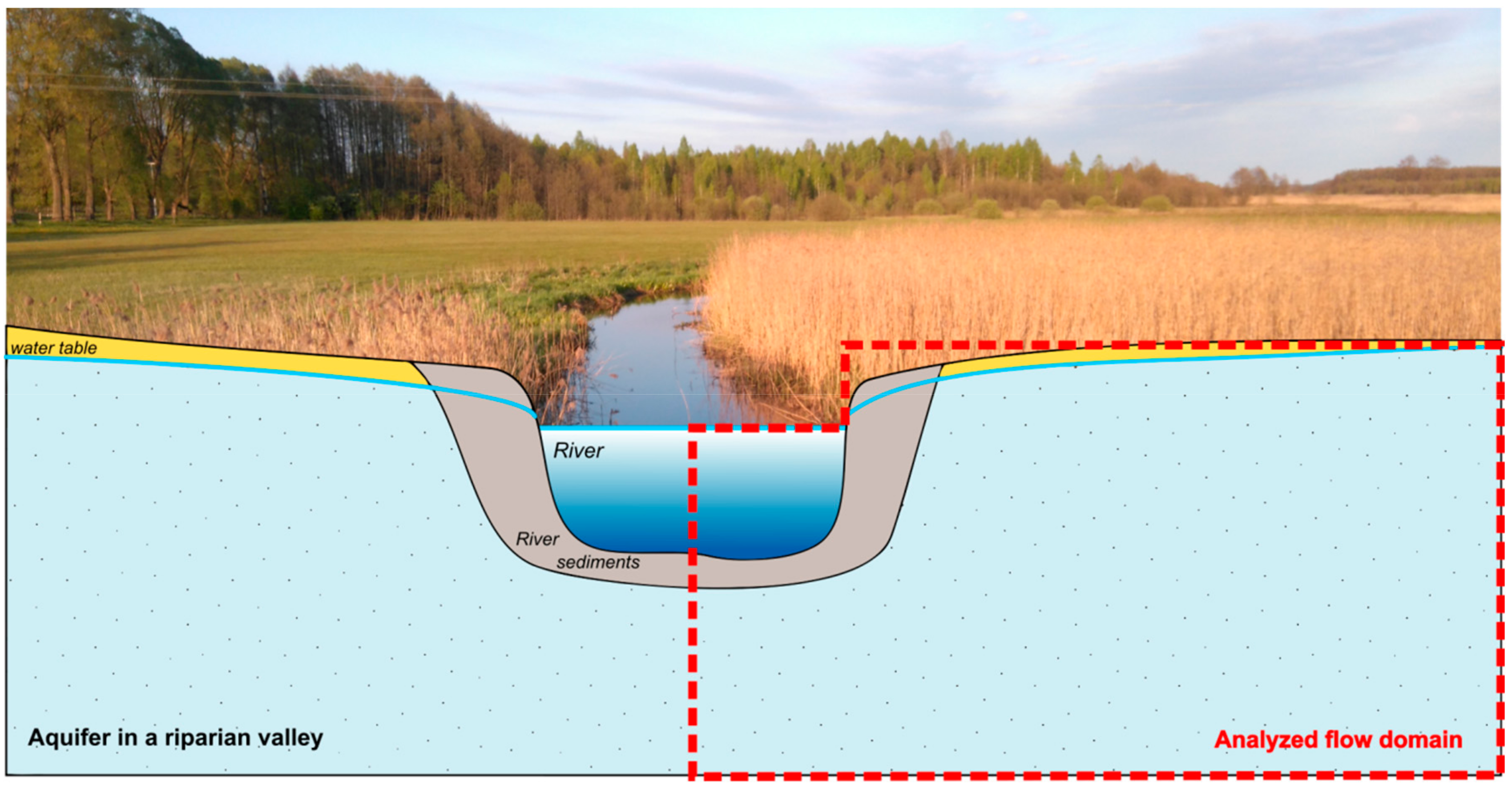
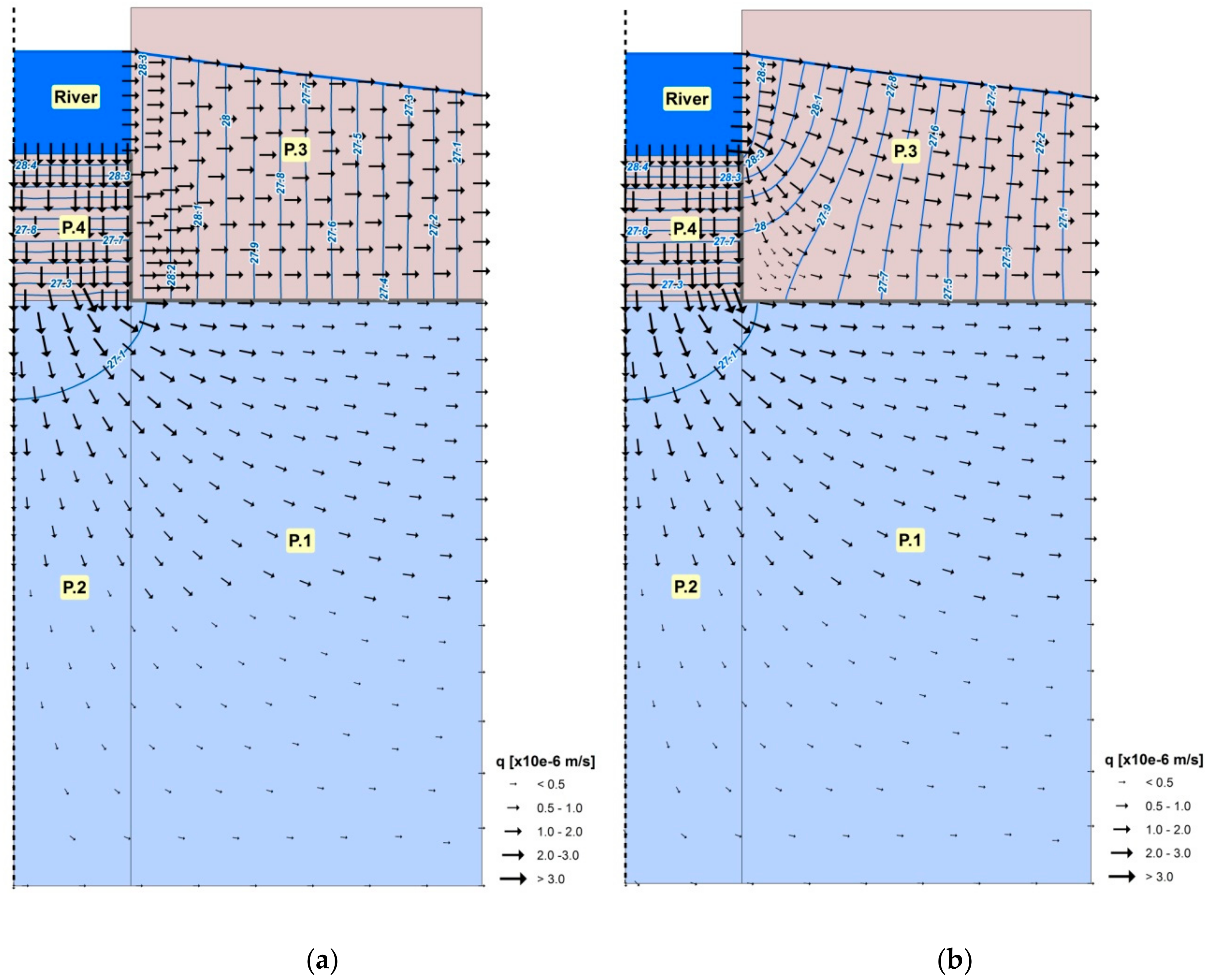
2.1. The Flow System

Water exchange between the river and aquifer occurs both through the river bottom and river banks. For rivers where L_bott >> L_bank (Figure 1a), vertical water seepage is the dominant part of total flow. For rivers where both lengths are comparable (Figure 1b), both streams are significant. Flow through the river banks should be particularly included in the description of the river–riparian aquifer water exchange in small rivers of the lowland landscape (e.g., the Upper Biebrza River in Poland) characterised by high depth relative to river width. The latter geometry is typical for small lowland rivers in agricultural regions in Poland. In the developed AHF model, allowing for calculation of the amount of water exchange in the hyporheic zone including vertical water seepage through the streambed and horizontal seepage through river banks, the geometry of the river cross-section and shape of river sediment is approximate with rectangle geometry. The analytical model of water exchange was developed with the assumption of simplified rectangular geometry of the riverbed cross-section (Figure 2).

Figure 3 illustrates the simplified geometry of the river–aquifer system and its relevant variables and parameters. For the sake of simplicity, the flow domain was subdivided into four subdomains, namely P.1, P.2, P.3, and P.4, each with a rectangular shape. Although the partition of the flow domain into simpler fragments is a relatively old method [20,27], it is still used in numerous cases to simplify the analytical approach [28], or in benchmarking of numerical models [29].

In the exemplary system, a vertically averaged (therefore constant) piezometric head in the riparian aquifer ${\Phi }^{*}$ along the right vertical boundaries of subdomains P.1 and P.3, and the height of water table in the river–$H_r$ are considered as external enforcing factor for water flow in the river–aquifer system.

The following dimensions are ascribed to river sediments of the river–aquifer system presented in Figure 3: D_a is the thickness of the aquifer beneath river sediments (m), W_rs is the half-width of river sediments (m), d_s is the thickness of river sediments below the river bottom (m), W_r is the half-width of the riverbed (m), L_ar is the one-side length of the riparian aquifer (m), D_ar is the maximum thickness of the riparian aquifer (m). The mineral bedrock beneath the riparian aquifer is adopted as the reference level for all variables. In the analytical model of groundwater flow in and under sediments, two state variables are defined: Φ_a(y) is the piezometric head in the semi-confined aquifer under the river sediments (m), h(y) is the height of free water table in river sediments of P.3 (m), h_s is the height of free water table in P.3 at the river bank (m). Aquifer and river sediments are also described in terms of their hydraulic parameters: $k_a$ is the hydraulic conductivity of aquifer under river sediments, i.e., in P.1 and P.2 (m/s), ${\mathrm{k}}_{\mathrm{s}}$ is the hydraulic conductivity of river sediments in P.3 and P.4 (m/s), $\mathrm{c}=\frac{{\mathrm{d}}_{\mathrm{s}}}{{\mathrm{k}}_{\mathrm{s}}}$ is the resistance to water flow in P.4 (s). Moreover, two variables describe external enforcing factors of the river is the aquifer system is the Figure 3: Φ^* is the averaged piezometric head in the riparian aquifer along the right vertical boundary of subdomains P.1 and P.3 (m), $H_r$ is the height of water table in the river (m). Two resultant variables are calculated by the AHF model: $Q_{bott}$ is the vertical seepage through the river bottom per 1 meter of the river stretch segment from/to flow domain P.2 (m³/s/m), $Q_{bank}$ is the horizontal seepage through the river bank per 1 meter of the river stretch segment from/to flow domain P.3 (m³/s/m).

Two halves of the river sedimentary envelope and two halves of a riparian valley—left (L) and right (R)—are neither physically nor geometrically identical. The model of seepage in river sediments and groundwater flow in the adjacent aquifer generally requires assessment of two different sets of parameters corresponding to L and R parts of the river–aquifer system. The assessment of the shape and location of a no-flow boundary between L and R parts of the system, however, is not possible with a simple analytical model considered in this article, because it requires solving a free boundary problem instead. In this article, river–aquifer water exchange is assessed by formulating an analytical model with only one set of identical parameters for the L and R sides of the flow system. Future stages of the research are planned to extend the present analytical model through relaxation of its most restrictive assumptions. The model is therefore anticipated to become suitable for more accurate assessment of water exchange with better approximation to the real flow system.

2.2. The AHF Model–Analytical Description of Water Seepage through River Sediments

Groundwater flow equations and their solutions used for calculating water exchange within different types of river–aquifer systems have been presented in the literature for a relatively long time. Water exchange through the river bottom has been in the focus of analytical models in a multitude of cases. A distinctive feature of the AHF model is simultaneous consideration of water exchange through sediments below the river bottom–P.4, and through sediments to the right of the river bank–P.3 (Figure 3). Several assumptions were made in order to simplify the analytical model of seepage in river sediments in terms of its physical adequacy and computational feasibility. The analytical model is aimed to ensure that the continuity of flow between the two water environments is fulfilled. The assumptions refer to geometry and processes in subdomains P.1 and P.2 of the aquifer under river sediments, and P.3, P.4 in river sediments. The simplifying assumptions for the AHF analytical model are as follows:

• Due to its slow dynamics, groundwater flow in and under river sediments can be approximated with a steady state flow. The assumption was analysed by Nawalany [30] who evidenced that despite a rapidly fluctuating river water table, a slow response of groundwater flow in the adjacent aquifer occurs as a consequence of dumping of high frequency changes in pore pressure by porous rocks. The adequacy of such an assumption was also discussed in more recent literature [26,31,32]. Preliminary field measurements in a real river–aquifer system show that water table fluctuations in the river–$H_r,$ and slow response of free water table that follows in the adjacent riparian aquifer–${\Phi }^{*}$ support the assumption of merely quasi-steady water exchange in the exemplary river–aquifer system. Both variables $H_r$ and ${\Phi }^{*}$ are used in the analytical AHF model as two independent external variables enforcing water flow in river sediments.
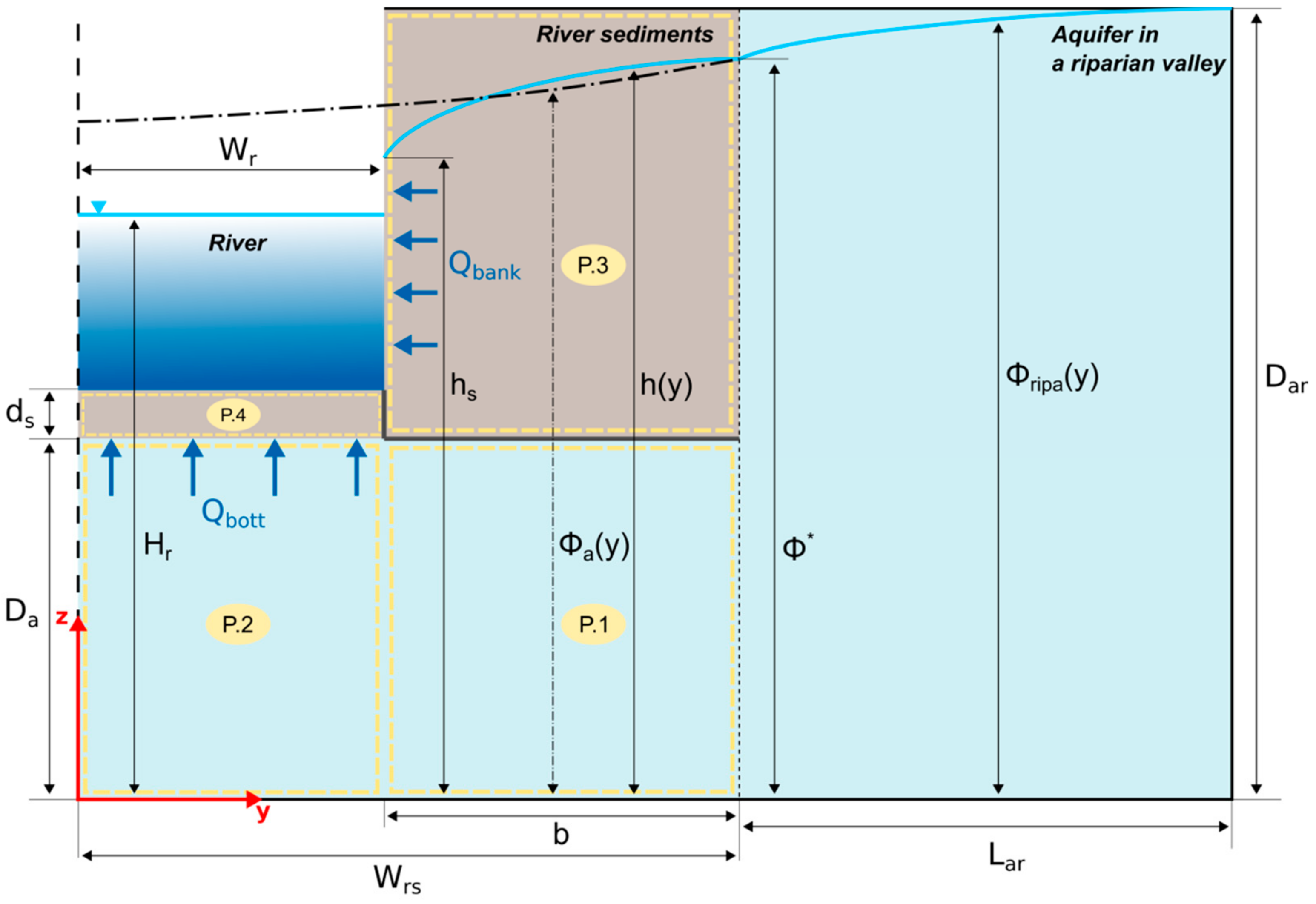
• The symmetry of the L and R parts of the river–aquifer system implies an existence of a no-flow boundary within the aquifer bellow river sediments. In the AHF model, this boundary is assumed to be a vertical line in the middle of the river. This rather restrictive simplification will be relaxed in the future developments of the model.
• Flow in subregion P.4 is assumed to be approximately vertical, because the left and the right boundaries of P.4 are vertical, whereas the upper boundary condition of the river water table is horizontal. Subregion P.4 is therefore described as a semi-pervious layer exerting a resistance drag (c) to water flowing from P.2 to the river bottom.
• Water flow between P.3 and P.4 is assessed as negligible. Therefore, the internal boundary between the two subregions is considered a no-flow boundary. The boundary between P.1 and P.3 is also assumed to be a no-flow boundary.
• The base of the river–aquifer system is impervious. Direct recharge of river sediments from the top by infiltrating precipitation is also assumed negligible.

Below flow in P.1, P.2, and P.3 parts of the river–aquifer system is described in terms of their boundary conditions, groundwater flow equations and their solutions, and respective parameters. Flow in subdomain P.4 is approximated by vertical seepage through the semi-pervious layer, and is linked to flow in P.2.

Flow in subdomain P.1 is confined and described by the Laplace equation:

$$k_a(\frac{{\partial }^2{\Phi }_a(y,z)}{\partial y^2}+\frac{{\partial }^2{\Phi }_a(y,z)}{\partial z^2})=0,\mathrm{for}y\in \left[W_r,W_{rs}\right],z\in \left[0,D_a\right]$$

(2)

with boundary conditions: left boundary is the horizontal component of specific discharge $-k_a\frac{\partial {\Phi }_a(W_r^{+},z)}{\partial y}$ equal to the horizontal component of specific discharge $-k_a\frac{\partial {\Phi }_a(W_r^{-},z)}{\partial y}$ at the vertical boundary between P.1 and P.2 and piezometric head continuous, i.e.,

$${\Phi }_a(W_r^{-},z)={\Phi }_a(W_r^{+},z)$$

(3)

right boundary is the imposed piezometric head (1st type b.c.), i.e.,

$${\Phi }_a(W_{rs},z)={\Phi }^{*}=const$$

(4)

lower boundary is the impervious boundary (2nd type b.c.), i.e.,

$$\frac{\partial {\Phi }_a(y,0)}{\partial z}=0$$

(5)

upper boundary is the no flow boundary (2nd type b.c.), i.e.,

$$\frac{\partial {\Phi }_a(y,D_a)}{\partial z}=0$$

(6)

because no water exchange is assumed between P.3 and P.1.

The solution to Equation (2) can be found by means of the factorisation method like in Nawalany‘s work [27], where some non-zero penetration of the riverbed into a confined aquifer $D_r>0$ was assumed. When $D_r$ converges to zero (as in the example of this article), the solution converges to

$$\begin{array}{c}{\tilde{\Phi }}_a(y,z)=\sum _{i=1}^{\infty }{D}_i\sinh [{\mu }_i(W_{rs}-y)]\cos ({\mu }_{i}z)+{\tilde{\Phi }}^{*}-{\beta }^{*}(W_{rs}-y)\\ \mathrm{for}y\in [W_r,W_{rs}],z\in [0,D_a]\end{array}$$

(7)

where

$${\tilde{\Phi }}_a(y,z)={\Phi }_a(y,z)-H_r$$

$${\tilde{\Phi }}^{*}={\Phi }^{*}-H_r$$

whereas its derivatives are equal to

$$\frac{\partial {\tilde{\Phi }}_a(y,z)}{\partial y}=-{\sum }_{i=1}^{\infty }{D}_i{\mu }_i\cosh [{\mu }_i(W_{rs}-y)]\cos ({\mu }_{i}z)+{\beta }^{*}$$

(8)

$$\frac{\partial {\tilde{\Phi }}_a(y,z)}{\partial z}=-{\sum }_{k=1}^{\infty }{D}_i{\mu }_i\sinh [{\mu }_i(W_{rs}-y)]\sin ({\mu }_{i}z).$$

(9)

Elements of series ($D_i),i=1,2\dots .$ and value of ${\beta }^{*}$ are derived further from requirements of flow continuity at the boundary between P.1 and P.2.

Solution of Equation (7) satisfies right b.c. as ${\tilde{\Phi }}_a(y=W_{rs},z)={\tilde{\Phi }}^{*}$ and, consistently, $\frac{\partial {\tilde{\Phi }}_a(y=W_{rs},z)}{\partial z}=0$ for all $z\in [0,D_a]$. For $y\in [W_r,W_{rs}],$ Equation (9) satisfies lower b.c., i.e., $\frac{\partial {\tilde{\Phi }}_a(y,z=0)}{\partial z}=0$. To also satisfy the no flow condition on the upper boundary of P.1, i.e., $\frac{\partial {\tilde{\Phi }}_a(y,z=D_a)}{\partial z}=0$, ${\mu }_i$ must be equal to

$${\mu }_i=\frac{i\pi }{D_a}\mathrm{for}i=1,2,\dots ,$$

(10)

Notice also that total outflow from P.1 into the riparian aquifer is equal to

$$\begin{array}{c}{Q}_{P.1\to rip}=-k_a{\int }_0^{D_a}\frac{\partial {\tilde{\Phi }}_a(y=W_{rs},z)}{\partial y}dz=k_a{\sum }_{i=1}^{\infty }{D}_i{\mu }_i{\int }_0^{D_a}\cos ({\mu }_{i}z)dz-\\ k_a{D}_a{\beta }^{*}=-k_a{D}_a{\beta }^{*}\end{array}$$

(11)

The minus sign in Equation (11) means that at that border, water physically flows along the x-axis if ${\beta }^{*}<0$, and opposite to y-axis if ${\beta }^{*}>0$.

Flow in subdomain P.2, i.e., in the part of the aquifer under river bottom sediments of P.4, is also described by the Laplace equation:

$$k_a(\frac{{\partial }^2{\Phi }_a(y,z)}{\partial y^2}+\frac{{\partial }^2{\Phi }_a(y,z)}{\partial z^2})=0\mathrm{for}y\in [0,W_r],z\in [0,D_a]$$

(12)

with boundary conditions: left boundary is the no flow boundary (2nd type b.c.), i.e.,

$$\frac{\partial {\Phi }_a(0,z)}{\partial y}=0$$

(13)

right boundary is the horizontal component of specific discharge $-k_a\frac{\partial {\Phi }_a(W_r^{-},z)}{\partial y}$ equal to horizontal component of specific discharge $-k_a\frac{\partial {\Phi }_a(W_r^{+},z)}{\partial y}$ at the vertical boundary between P.2 and P.1, and also piezometric head is continuous, i.e.,

$${\Phi }_a(W_r^{-},z)={\Phi }_a(W_r^{+},z)$$

(14)

lower boundary is the impervious boundary (2nd type b.c.), i.e.,

$$\frac{\partial {\Phi }_a(y,0)}{\partial z}=0$$

(15)

upper boundary is the seepage through a layer of river sediments of P.4 to river bottom, i.e.,

$$q_s=-k_a\frac{\partial {\Phi }_a(y,D_a)}{\partial z}=\frac{{\Phi }_a(y,D_a)-H_r}{c}$$

(16)

The solution to the flow Equation (12) in P.2 satisfying b.c.-s, Equations (13)–(16), can be found by means of the factorisation method. It is given by the following formula

$${\Phi }_a(y,z)=H_r+{\sum }_{k=1}^{\infty }{A}_k\cosh ({\lambda }_{k}y)\cos ({\lambda }_{k}z),\mathrm{for}y\in [0,W_r],z\in [0,D_a]$$

(17)

whereas its derivatives are equal to

$$\frac{\partial {\Phi }_a(y,z)}{\partial y}={\sum }_{k=1}^{\infty }{A}_k{\lambda }_k\sinh ({\lambda }_{k}y)\cos ({\lambda }_{k}z)$$

(18)

$$\frac{\partial {\Phi }_a(y,z)}{\partial z}=-{\sum }_{k=1}^{\infty }{A}_k{\lambda }_k\cosh ({\lambda }_{k}y)\sin ({\lambda }_{k}z)$$

(19)

Parameters ${\lambda }_k$ are specified through b.c. (16)

$$-k_a\frac{\partial {\Phi }_a(y,D_a)}{\partial z}=\frac{{\Phi }_a(y,D_a)-H_r}{c}\equiv -\frac{\partial {\tilde{\Phi }}_a(y,D_a)}{\partial z}=\frac{{\tilde{\Phi }}_a(y,D_a)}{{\chi }^2}$$

(20)

$$\mathrm{where}{\tilde{\Phi }}_a(y,z)={\Phi }_a(y,z)-H_r\mathrm{and}{\chi }^2=k_{a}c$$

(21)

Substituting Equation (17) and Equation (19) to Equation (20) provides ${\sum }_{k=1}^{\infty }{A}_k{\lambda }_k{\chi }^2\cosh ({\lambda }_{k}y)\mathrm{tg}({\lambda }_k{D}_a)\cos ({\lambda }_k{D}_a)={\sum }_{k=1}^{\infty }{A}_k\cosh ({\lambda }_{k}y)\cos ({\lambda }_k{D}_a)=>$ ${\lambda }_k{\chi }^2\mathrm{tg}({\lambda }_k{D}_a)=1$ Elements of series $({\lambda }_k),k=1,\dots$ can be calculated from the non-linear algebraic equation

$$\frac{D_a}{{\chi }^2}\frac{1}{{\tilde{\lambda }}_k}=tg({\tilde{\lambda }}_k)$$

(22)

$$\mathrm{where}{\tilde{\lambda }}_k={\lambda }_k{D}_a$$

(23)

for instance by the Newton method.

Elements of series $(A_k),k=1,2,\dots$ are derived below from the requirements of continuity along the vertical boundary between P.1 and P.2. Once parameters $A_k$ and ${\lambda }_k$ are known,$Q_{bott}$ can be calculated from Equation (19) by integrating specific discharge $q_z$ over top horizontal boundary of subregion P.2, i.e.,

$$Q_{bott}={\int }_0^{W_r}{q}_z(y,D_a)dy={\int }_0^{W_r}-k_a\frac{\partial {\Phi }_a\left(y,D_a\right)}{\partial z}dy=k_a{\sum }_{k=1}^{\infty }{A}_k{\lambda }_k\sin ({\lambda }_k{D}_a){\int }_0^{W_r}\cosh ({\lambda }_{k}y)dy$$

(24)

hence

$$Q_{bott}=k_a{\sum }_{k=1}^{\infty }{A}_k\sin ({\lambda }_k{D}_a)\sinh ({\lambda }_k{W}_r),({\mathrm{m}}^3/\mathrm{s}/\mathrm{m})$$

(25)

Flow continuity between subregion P.1 and P.2. In order to evaluate elements of series $(A_k),k=1,2,\dots$, $(D_i),i=1,2,\dots$ and value of ${\beta }^{*}$, the piezometric head and horizontal components of specific discharge must be assumed continuous along the boundary between flow subregions P.1 and P.2, i.e., at $y=W_r$ and for $z\in [0,D_a]$

$${\sum }_{k=1}^{\infty }{A}_k\cosh ({\lambda }_k{W}_r)\cos ({\lambda }_{k}z)={\sum }_{i=1}^{\infty }{D}_i\sinh [{\mu }_i(W_{rs}-W_r)]\cos ({\mu }_{i}z)+{\tilde{\Phi }}^{*}-{\beta }^{*}(W_{rs}-W_r)$$

(26)

$${\sum }_{k=1}^{\infty }{A}_k{\lambda }_k\sinh ({\lambda }_k{W}_r)\cos ({\lambda }_{k}z)=-{\sum }_{i=1}^{\infty }{D}_i{\mu }_i\cosh [{\mu }_i(W_{rs}-W_r)]\cos ({\mu }_{i}z)+{\beta }^{*}$$

(27)

Once elements of series $(A_k$)$,k=1,2$…are known, value of ${\beta }^{*}$ can be calculated from mass conservation in flow subregions P.1 and P.2, i.e., from equality of Equations (11) and (25)

$$\begin{array}{c}{\mathrm{Q}}_{\mathrm{P}.1\to \mathrm{rip}}={\mathrm{Q}}_{\mathrm{bott}}\equiv -{\mathrm{k}}_{\mathrm{a}}{\mathrm{D}}_{\mathrm{a}}{\mathsf{\beta }}^{*}={\mathrm{k}}_{\mathrm{a}}{\sum }_{\mathrm{k}=1}^{\infty }{\mathrm{A}}_{\mathrm{k}}\sin ({\mathsf{\lambda }}_{\mathrm{k}}{\mathrm{D}}_{\mathrm{a}})\sinh ({\mathsf{\lambda }}_{\mathrm{k}}{\mathrm{W}}_{\mathrm{r}})\equiv \\ {\mathsf{\beta }}^{*}=-{\sum }_{\mathrm{k}=1}^{\infty }{\mathrm{A}}_{\mathrm{k}}\sin ({\mathsf{\lambda }}_{\mathrm{k}}{\mathrm{D}}_{\mathrm{a}})\sinh ({\mathsf{\lambda }}_{\mathrm{k}}{\mathrm{W}}_{\mathrm{r}})/{\mathrm{D}}_{\mathrm{a}}\end{array}$$

(28)

To evaluate elements of the two series, $(A_k$), $k=1,2$… and $\left(D_i\right)$, $i=1,2\dots$, equality (6.2) needs to be multiplied by $b=\left(W_{rs}-W_r\right)$ and added to Equation (26), resulting in

$$\begin{array}{c}{\sum }_{k=1}^{\infty }{A}_k\left[\cosh \left({\lambda }_k{W}_r\right)+{\lambda }_{k}b\sinh \left({\lambda }_k{W}_r\right)\right]\cos \left({\lambda }_{k}z\right)=\\ ={\sum }_{j=1}^{j=\infty }{D}_j[\sinh \left({\mu }_{j}b\right)-{\mu }_{j}b\cos \mathrm{h}\left({\mu }_{j}b\right)]\cos \left({\mu }_{j}z\right)+{\tilde{\Phi }}^{*}\end{array}$$

(29)

Ultimately, values of $\left(2N+2\right)$ unknowns—$(A_k$), $k=1,2\dots ,\left(N+1\right)$,$\left(D_i\right)$, $i=1,2\dots ,\left(N+1\right)$—need to be found. Simultaneous substitution of Equation (28) for ${\beta }^{*}$ and $z_m=\frac{m{D}_a}{N},m=0,1\dots ,N$ for $z$ into Equations (26) and (27) leads to a set of $\left(2N+2\right)$ linear algebraic equations, where infinite series are approximated with their finite counterparts

$$\begin{array}{c}{\sum }_{k=1}^{N+1}{A}_k\{\cosh ({\lambda }_k{W}_r)\cos ({\lambda }_k{z}_m)-\frac{b}{D_a}sin({\lambda }_k{D}_a)\sinh ({\lambda }_k{W}_r)\}-\\ {\sum }_{i=1}^{N+1}{D}_i\sinh [{\mu }_{i}b]\cos ({\mu }_i{z}_m)={\tilde{\Phi }}^{*},m=0,1,\dots ,N\end{array}$$

(30)

$$\begin{array}{c}{\sum }_{k=1}^{N+1}{A}_k\{{\lambda }_k\sinh ({\lambda }_k{W}_r)\cos ({\lambda }_k{z}_m)+sin({\lambda }_k{D}_a)sinh({\lambda }_k{W}_r)/D_a\}+\\ +{\sum }_{i=1}^{N+1}{D}_i{\mu }_i\cosh [{\mu }_{i}b]\cos ({\mu }_i{z}_m)=0,m=0,1,\dots ,N\end{array}$$

(31)

Hyperbolic sine and cosine in Equations (30) and (31) need some pre-calculation to avoid rising exponents, i.e., $sinh\alpha =exp\alpha$ [$1-exp\left(-2\alpha \right)]/2$ and $cosh\alpha =\exp \alpha$ [$1+exp\left(-2\alpha \right)]/2$. By denoting

$$\widehat{A_k}=A_{k}exp({\lambda }_k{W}_r)$$

(32)

$${\widehat{D}}_i=D_{i}exp({\mu }_{i}b)$$

(33)

• ${\tilde{\omega }}_{mk}=\{\cos \left({\lambda }_k{z}_m\right)-\frac{b}{D_a}sin\left({\lambda }_k{D}_a\right)tgh\left({\lambda }_k{W}_r\right)\}\left[1+exp\left(-2{\lambda }_k{W}_r\right)\right]/2$
• ${\tilde{\tilde{\omega }}}_{mk}=\left\{\{{\lambda }_k\cos \left({\lambda }_k{z}_m\right)+\frac{sin\left({\lambda }_k{D}_a\right)}{D_a}\right\}\left[1-exp\left(-2{\lambda }_k{W}_r\right)\right]/2$
• ${\tilde{\delta }}_{mi}=-\cos \left({\mu }_i{z}_m\right)\left[1-exp\left(-2{\mu }_{i}b\right)\right]/2$
• ${\tilde{\tilde{\delta }}}_{mi}={\mu }_i\cos \left({\mu }_i{z}_m\right)\left[1+exp\left(-2{\mu }_{i}b\right)\right]/2$

Equations (30) and (31) can be written shortly as

$${\sum }_{k=1}^{N+1}\widehat{A_k}{\tilde{\omega }}_{mk}-{\sum }_{i=1}^{N+1}{\widehat{D}}_i{\tilde{\delta }}_{mi}={\tilde{\Phi }}^{*},m=0,1,\dots ,N$$

(34)

$${\sum }_{k=1}^{N+1}\widehat{A_k}{\tilde{\tilde{\omega }}}_{mk}+{\sum }_{i=1}^{N+!}{\widehat{D}}_i{\tilde{\tilde{\delta }}}_{mi}=0,m=0,1,\dots ,N$$

(35)

or in the block-matrix form for as

$$\left[\frac{{\tilde{\Omega }}_{\left(N+1\right)x\left(N+1\right)}|}{{\tilde{\tilde{\Omega }}}_{\left(N+1\right)x\left(N+1\right)}|}\frac{{\tilde{\Delta }}_{\left(N+1\right)x\left(N+1\right)}}{{\tilde{\tilde{\Delta }}}_{\left(N+1\right)x\left(N+1\right)}}\right]\left[\frac{{\widehat{A}}_{\left(N+1\right)x1}}{{\widehat{D}}_{\left(N+1\right)x1}}\right]=\left[{{\rm P}}_{\left(2N+2\right)x1}\right]$$

(36)

where

• ${\tilde{\Omega }}_{\left(N+1\right)x\left(N+1\right)}=\left\{{\tilde{\omega }}_{mk}\right\}\left(m=0,1,\dots ,N;k=1,\dots ,N+1\right)$
• ${\tilde{\tilde{\Omega }}}_{\left(N+1\right)x\left(N+1\right)}=\left\{{\tilde{\tilde{\omega }}}_{mk}\right\}\left(m=0,1,\dots ,N;k=1,\dots ,N+1\right)$
• ${\tilde{\Delta }}_{\left(N+1\right)x\left(N+1\right)}=\left\{{\tilde{\delta }}_{mk}\right\}\left(m=0,1,\dots ,N;k=1,\dots ,N+1\right)$
• ${\tilde{\tilde{\Delta }}}_{\left(N+1\right)x\left(N+1\right)}=\left\{{\tilde{\tilde{\delta }}}_{mk}\right\}\left(m=0,1,\dots ,N;k=1,\dots ,N+1\right)$
• ${\widehat{A}}_{\left(N+1\right)x1}=\left[\widehat{A_k}\right]\left(k=1,\dots ,N+1\right)$ is the first (sub)vector of unknowns
• ${\widehat{D}}_{\left(N+1\right)x1}=\left[{\widehat{D}}_i\right]\left(i=1,\dots ,N+1\right)$ is the second (sub)vector of unknowns
• ${{\rm P}}_{\left(2N+2\right)x1}=[\begin{array}{c}\underset{\_}{{\tilde{\Phi }}^{*}}\\ \underset{\_}{0}\end{array}]$ is the right hand side vector.

After solving Equation (36) for $(A_k$)$,k=1,2\dots ,\left(N+1\right)$, the sought seepage through river bottom is the $Q_{bott}$ can be readily calculated from approximations of Equation (11) or (24)

$$Q_{bott}=-k_a{D}_a{\beta }^{*}\mathrm{or}$$

(37)

$$Q_{bott}=k_a\sum _{k=1}^{N+1}{A}_k\sin \left({\lambda }_k{D}_a\right)\sinh \left({\lambda }_k{W}_r\right)=k_a\sum _{k=1}^{N+1}\widehat{A_k}\sin \left({\lambda }_k{D}_a\right)\left[1-exp\left(-2{\lambda }_k{W}_r\right)\right]/2$$

(38)

Convergence of finite series $(A_k),k=1,2\dots ,\left(N+1\right)$ and $\left(D_i\right),i=1,2\dots ,\left(N+1\right)$ has been checked for increasing $N$.

Flow through river sediments in subdomain P.3 is unconfined and, after moving the origin of coordinates to point $\left(y_o=W_r,z_o=D_a\right),$ described by the Laplace equation

$$k_s(\frac{{\partial }^2{\Phi }_s(y,z)}{\partial y^2}+\frac{{\partial }^2{\Phi }_s(y,z)}{\partial z^2})=0,\mathrm{for}y\in [0,b],z\in [0,h(y)]$$

(39)

where

${\Phi }_s\left(y,z\right)=\Phi \left(y,z\right)-D_a$ is the piezometric head in sediments of P.3 (m),

$b=W_{rs}-W_r$ is the width of P.3 (m),

$h\left(y\right):=h\left(y\right)-D_a$ is the height of free water table in P.3 over the reference level $z_0=D_a$, (m)

with boundary conditions at:

left boundary consisting of three segments: (assumed) no-flow boundary between P.3 and P.4 (2nd type b.c.), i.e., $\frac{\partial {\Phi }_s\left(0,z\right)}{\partial y}=0,0\le z\le d_s$, constant head along the water part of the river bank (1st type b.c.), i.e., ${\varphi }_s\left(0,z\right)=H_r$, $d_s<z\le H_r$, seepage face $h_s$ along the aerial part of the river bank (1st type b.c.), i.e.,

$${\varphi }_s\left(0,z\right)=z,H_r<z\le h_s=h\left(0\right)$$

(40)

right boundary is the constant piezometric head (1st type b.c.), i.e.,

$${\varphi }_s\left(b,z\right)={\varphi }^{*},0\le z\le {\varphi }^{*}$$

(41)

lower boundary is the (assumed) no flow boundary between P.1 and P.3 (2nd type b.c.), i.e.,

$$\frac{\partial {\varphi }_s\left(y,0\right)}{\partial z}=0,0\le y\le b$$

(42)

upper boundary is the free boundary of P.3, i.e., ${\varphi }_s\left(y,h\left(y\right)\right)=h\left(y\right)$ with no recharge from the top i.e.,

$$\frac{\partial {\varphi }_s\left(y,h\left(y\right)\right)}{\partial z}=0,0\le y\le b$$

(43)

External constraints are also referenced to $z_0=D_a$, i.e., $H_r:=H_r-D_a$ and ${\varphi }^{*}:={\varphi }^{*}-D_a$.

Because the height of free water table $h\left(y\right)$ in P.3 is unknown, and so is the height of seepage face $h_s=h\left(0\right)$, algebraic relationship ${\varphi }_s\left(y,h\left(y\right)\right)=h\left(y\right)$ is added to make the solution to Equation (39) unique. The unknown shape of subregion P.3 makes the problem Equations (39)–(43) into a free boundary issue, and is cumbersome to solve. The calculation of river inflow/outflow to/from subregion P.3,$Q_{bank}$, however, is possible by means of the method originally derived by Czarny [23]. It allows for calculating unconfined flow in sediments of subdomain P.3 without actual solving of the free boundary problem Equations (39)–(43). By applying Leibnitz theorem to Darcy’s Law, the following general formula for total flow in P.3, $Q_s\left(y\right),$ can be derived

$$\begin{array}{c}{Q}_s\left(y\right)={\int }_0^{h\left(y\right)}[-k_s\frac{\partial {\Phi }_s\left(y,z\right)}{\partial y}]dz=-k_s\frac{\partial }{\partial y}\{{\int }_0^{h\left(y\right)}{\Phi }_s\left(y,z\right)dz-\frac{{[h\left(y\right)]}^2}{2}\}=\\ =-k_s\frac{\partial }{\partial y}\{h\left(y\right)\tilde{\Phi }\left(y\right)-\frac{{[h\left(y\right)]}^2}{2}\}\end{array}$$

(44)

where $\tilde{\Phi }\left(y\right)=\frac{1}{h\left(y\right)}{\int }_0^{h\left(y\right)}{\Phi }^s\left(y,z\right)dz$ is the average piezometric head in river sediments of P.3 along any arbitrary vertical at $y$ over the assumed reference level at $z_0=D_a$.

Equation (44) has been originally derived by Czarny [23] to justify the use of the Dupuit parabola when calculating inflow of groundwater to an excavation. In this article, the Czarny method is slightly generalised by considering a no-flow boundary at lower part of the left vertical boundary of P.3 (see Equation (40)).

Because there is neither seepage from P.1 to P.3 nor recharge from the top, the continuity of flow in P.3 requires that $\frac{\partial Q_s\left(y\right)}{\partial y}=0$, and therefore

$$\frac{{\partial }^2}{\partial y^2}\left[h\left(y\right)\tilde{\Phi }\left(y\right)-\frac{{[h\left(y\right)]}^2}{2}\right]=0$$

(45)

The general solution to this equation can be proposed in a simple form

$$h\left(y\right)\tilde{\Phi }\left(y\right)-\frac{{[h\left(y\right)]}^2}{2}=A{y}^2+By+C$$

(46)

Substitution of parabola, Equation (46) to Equation (45) results in $A=0,$ and therefore

$$h\left(y\right)\tilde{\Phi }\left(y\right)-\frac{{[h\left(y\right)]}^2}{2}=By+C$$

(47)

whereas the sought total flow at any $y$ can be calculated from Equation (44), i.e.$,Q_s\left(y\right)=-k_{s}B$.

Constants B and C can be assessed from the assumed boundary conditions at the P.3 left and right boundaries, namely for y = 0: $h\left(0\right)\tilde{\Phi }\left(0\right)-\frac{{[h\left(0\right)]}^2}{2}=C$, where $h\left(0\right)=h_s$, whereas term $h\left(0\right)\tilde{\Phi }\left(0\right)$ at the river bank is equal to

$$h\left(0\right)\tilde{\Phi }\left(0\right)={\int }_0^{h\left(0\right)}{\Phi }_s\left(0,z\right)dz={\int }_0^{d_s}{\Phi }_s\left(0,z\right)dz+{\int }_{d_s}^{H_r}{\Phi }_s\left(0,z\right)dz+{\int }_{H_r}^{h_s}{\Phi }_s\left(0,z\right)dz.$$

(48)

The first integral can be derived from the observation that for ${\varphi }^{*}>H_r$,piezometric head along the flowline located at lower no-flow horizontal part of P.3 boundary, i.e., at $z=0\left(z_0=D_a\right),$ and continuing further along the no-flow lower part of the left vertical boundary of P.3 at $y=0,$ changes linearly from ${\varphi }^{*}$ down to $H_r$. Therefore, for $0\le z\le d_s,{\varphi }_s\left(0,z\right)=H_r+\frac{{\varphi }^{*}-H_r}{b+d_s}(d_s-z,)$ and hence ${\int }_0^{d_s}{\varphi }_s\left(0,z\right)dz=H_r{d}_s+\frac{{\varphi }^{*}-H_r}{b+d_s}\frac{d_s^2}{2}$. Using b.c. Equation (40) for other parts of the left boundary of P.3, the remaining two integrals can be calculated, ${\int }_{d_s}^{H_r}{\varphi }_s\left(0,z\right)dz=H_r\left(H_r-d_s\right)$ and ${\int }_{H_r}^{h_s}{\varphi }_s\left(0,z\right)dz=\frac{h_s^2-H_r^2}{2}.$ Adding the three integrals of Equation (48) provides $C=h\left(0\right)\tilde{\Phi }\left(0\right)-\frac{{[h\left(0\right)]}^2}{2}=\frac{H_r^2}{2}+\frac{{\Phi }^{*}-H_r}{b+d_s}\frac{d_s^2}{2}$. For y =$b$: $h\left(b\right)\tilde{\varphi }\left(b\right)-\frac{{\left[h\left(b\right)\right]}^2}{2}=Bb+C⟹{\varphi }^{*}{\varphi }^{*}-\frac{{\left[{\varphi }^{*}\right]}^2}{2}=Bb+C⟹B=\frac{\{\frac{{\left[{\varphi }^{*}\right]}^2}{2}-\frac{H_r^2}{2}-\frac{{\varphi }^{*}-H_r}{b+d_s}\frac{d_s^2}{2}\}}{b},$ and therefore one-side

$$Q_{bank}=Q_s\left(y=0\right)=-k_{s}B=-\frac{k_s}{2b}\left\{{[{\Phi }^{*}]}^2-H_r^2-\frac{{\Phi }^{*}-H_r}{b+d_s}{d}_s^2\right\}$$

(49)

For ${\Phi }^{*}>H_r,Q_{bank}<0$, which indicates inflow to the river from P.3.

For $H_r>{\Phi }^{*},$ flow reverses, and there is no seepage face either at the left nor at the right boundary of P.3, i.e.,$h\left(0\right)=H_r$ and $h\left(b\right)=\tilde{\Phi }\left(b\right)={\Phi }^{*}$. Then, total flow, Equation (44) can be evaluated from two integrals of Equation (48) -${\int }_0^{d_s}{\Phi }^s\left(0,z\right)dz$ and ${\int }_{d_s}^{H_r}{\Phi }^s\left(0,z\right)dz,$ as

$$Q_{bank}=\frac{k_s}{2b}\left\{H_r^2-{[{\Phi }^{*}]}^2-\frac{H_r-{\Phi }^{*}}{b+d_s}{d}_s^2\right\}$$

(50)

After moving back to the original global of coordinates $\left(y_o=0,z_o=0\right),$ Equations (49) and (50) can be shortly written as:

$$Q_{bank}=\frac{k_s}{2b}\left\{{\left(H_r-D_a\right)}^2-{\left({\varphi }^{*}-D_a\right)}^2-\frac{H_r-{\varphi }^{*}}{b+d_s}{d}_s^2\right\}$$

(51)

When $d_s=0$, Equation (51) reduces to the Dupuit formula $Q_{bank}=\frac{k_s}{2b}$ ${\{(H_r-D_a)}^2-{[{\Phi }^{*}]}^2{({\varphi }^{*}-D_a)}^2\}$.

Ultimately, through adding formulae of outflow/inflow from/to riparian aquifer to/from a river through its bottom— Equation (37) or (38)—and bank— Equation (51)—the total one side river recharge per 1 m of the river segment can be calculated as follows:

$$Q_{total}=Q_{bottom}+Q_{bank},({\mathrm{m}}^3/\mathrm{s}/\mathrm{m})$$

(52)

2.3. The SEEP2D Model–Numerical Approximation of Water Seepage in the River–Aquifer System

River–aquifer water exchange calculated with the AHF analytical model can be compared with the corresponding water flows approximated by SEEP2D software suitable for modelling a variety of problems involving seepage. The SEEP2D is a 2D finite element, steady state, flow model successfully applied in cross-section (profile) models representing a vertical slice through a flow system such as earth dams or levees. The SEEP2D model is based on the Equation (53) [33].

$$\frac{\partial }{\partial y}\left(K_{yy}\frac{\partial h}{\partial y}+K_{yz}\frac{\partial h}{\partial z}\right)+\frac{\partial }{\partial z}\left(K_{zz}\frac{\partial h}{\partial z}+K_{zy}\frac{\partial h}{\partial y}\right)=0$$

(53)

where h is the total head (elevation head plus pressure head), K is the hydraulic conductivity tensor.

SEEP2D permits modelling for the following conditions: isotropic and anisotropic soil properties; confined and unconfined flow for cross-section models; saturated/unsaturated flow for unconfined cross-section models; flow simulation in saturated and unsaturated zones; heterogeneous soil conditions. In the model, the Laplace Equation (53) is solved by means of the finite element method (FEM), and the flow domain is represented by a finite element mesh consisting of triangular and quadrilateral elements. In unconfined problems, where the position of the free surface of water is unknown, SEEP2D allows for modelling of either the deformation of the mesh to the phreatic surface, or simulation of flow in both saturated and unsaturated zones. In the first approach, flow occurs only in the saturated zone, and is iteratively finding the location of the phreatic surface. The mesh is deformed or truncated for the upper boundary of the mesh to match the phreatic surface. When unsaturated flow is simulated, hydraulic conductivity is modified using either the linear frontal method or the Van Genuchten method [34]. The following boundary conditions can be used in the model at the node in the mesh: constant head (Dirichlet boundary condition), head equals the elevation (exit face), flow rate. Known flux rate is used as a boundary condition along a sequence of element edges on the perimeter of the flow domain. Exit face boundary conditions are used when simulating unconfined flow problems, and should be added along the face where the free surface is likely to exit the flow domain. The SEEP2D program calculates the head, flow, discharge (Darcian) velocity, and pore pressure at every node in the mesh. In the example of water seepage considered in this article, the flow domain-2D cross-section-a vertical slice through a flow system, (Figure 3) and flow condition–unconfined flow in the saturated zone, permit applying the SEEP2D model with the deforming mesh option.

3. Simulation Results and Discussion

Six scenarios of the difference in the mutual position of the water table in the aquifer and river were selected for analysis. The initial scenario, considered the most common, is scenario 3 and 4 (0.5 m difference between Φ^* and H_r for the gaining/losing type of river). Such differences are observed for small and deep lowland rivers (e.g., the Upper Biebrza River in Poland). During the drainage period, the difference between Φ^* and H_r is approximately 0.5 m during infiltration periods, the difference reaches maximum 2 m. Other scenarios were selected to test models in a wide range of differences between H_r and Φ^* both when the river is of draining and infiltrating type.

Parameter values presented in

Table 1. Parameters of river sediments, riverbed, and riparian aquifer in the exemplary system.

Variable	Values
Da	20 m
ka	0.000116 m/s
Wrs	16 m
Wr	4 m
ds	5 m
ks	0.00001 m/s
Hr	25.5–28.5 m
Φ*	27 m

were used for calculating water exchange flows by means of the AHF and SEEP2D models for the exemplary river–aquifer system. These parameters were estimated based on of the real river–aquifer system of the Upper Biebrza River in Poland.

Performing the simulation with the AHF model requires acquiring the variables listed in Table 1. In addition to the knowledge of the hydraulic parameters, the application of SEEP2D software for calculations requires the development of a 2D finite element mesh for the flow domain. In the calculation example, a finite element mesh representing the river–aquifer system flow domain (Figure 3) was generated with mesh generation tools provided in GMS Groundwater Modelling System. In the model, the “no-flow” boundary was applied to the bottom of the aquifer system. Constant head boundary conditions are in locations where the head and river water table are known. The fixed value of groundwater table in the riparian aquifer Φ^* (Figure 3) along the left and right perimeter of the flow domain (where nodes elevation is not greater then Φ^*), and fixed value of river table along the wetted perimeter in the banks and bottom of the river. When river is of the gaining type (H_r < 27 m) exit face boundary conditions are placed along the river perimeter (left and right river bank above the water table). When the river is of the losing type (H_r > Φ^*), exit face boundary conditions are placed along the left and right perimeter of the flow domain in nodes with an elevation greater than Φ^*. In the remaining part of the perimeter of the flow domain, the “no-flow” boundary conditions are assumed.

In calculations where SEEP2D reflected the simplifying assumptions made in the AHF model, the boundary conditions are implemented by placing constant head boundary conditions in locations where the head and river water are known, and “no-flow” boundary conditions on the remaining part of the perimeter of the flow domain (the same boundary conditions were applied as in the AHF model). The assumption of no flow between P.3 and P.4 as well as between P.1 and P.3 (Figure 3) was implemented in SEEP2D software by creating a discontinuity in the mesh—an impermeable flow barrier with a width of 0.05 m—and placing “no-flow” boundary conditions in nodes along the outer perimeter of this barrier.

In the case of exit face boundary conditions, if the head at a node on the boundary becomes greater than the node elevation during the iteration process, the head at the node is fixed at the nodal elevation and the node acts as a specified head boundary. In the calculation, the SEEP2D software was used with the deforming mesh option (unconfined flow in the saturated zone). In this case, the boundary conditions are implemented by placing constant head boundary conditions in locations where the head and river water table are known, and iteratively is finding the location of the phreatic surface, and the mesh is deformed or truncated so that the upper boundary of the mesh matches the phreatic surface, placing exit face boundary conditions along the boundary where the phreatic surface is assumed to exit.

The basic finite element mesh in the SEEP2D model consist of 1185 nodes and 2127 triangle elements. It was refined in an area of sediment close to river banks and bottom, with high flow or high gradient in head. The mesh element size along the river cross-section is Δx = 0.25 m. To ensure a suitable mesh size, test calculations were performed for a twice denser mesh (4564 nodes and 8508 elements, Δx = 0.125 m). A test with decreasing density of the mesh (522 nodes, 944 elements, Δx = 0.5 m) was also performed. Calculation was done for all scenarios presented in

Table 2. Impact of finite element mesh size on calculated river recharge/discharge through groundwater seepage (A, 1185 nodes; B, 4564 nodes; C, 522 nodes).

Scenario No.	Qtot [×10−6 m3/s/m]			B/A	C/A
	MESH
	A	B	C
1	−39.7	−39.5	−39.8	0.9951	1.0027
2	−27.4	−27.3	−27.6	0.9955	1.0057
3	−14.2	−14.1	−14.2	0.9956	1.0026
4	14.9	14.8	15.0	0.9949	1.0026
5	30.3	30.2	30.5	0.9967	1.0050
6	46.4	46.2	46.6	0.9961	1.0041

. The estimated differences in calculated flow across the river bottom and banks for the base, refine, and decrease finite element mesh are in a range from 0.27% to 0.57%. These test results show that the base finite element mesh in SEEP2D model has a suitable mesh size.

The results of the analytical AHF model in terms of Q_bank, Q_bott, and Q_tot are listed in

Table 3. One side $Q_{bank},Q_{bott}$, and $Q_{tot}$ assessed by means of the analytical (AHF) and numerical (SEEP2D) models (with assumption of no flow between P.3–P.4 and P.1–P.3).

Scenario No.	Φ*[m]	Hr[m]	Qbank, Qbott, Qtot [×10−6 m3/s/m] 1
			AHF			SEEP2D
			Qbank	Qbott	Qtot	Qbank	Qbott	Qtot
1	27.0	25.5	−6.89	−10.76	−17.65	−5.39	−10.56	−15.95
2	27.0	26.0	−4.80	−7.17	−11.97	−3.94	−7.04	−10.98
3	27.0	26.5	−2.51	−3.58	−6.09	−2.13	−3.52	−5.65
4	27.0	27.5	2.71	3.58	6.29	2.40	3.52	5.92
5	27.0	28.0	5.64	7.17	12.81	5.02	7.04	12.06
6	27.0	28.5	8.77	10.76	19.53	7.87	10.56	18.43

¹ negative values indicate the river is recharged by riparian aquifer groundwater through river sediments and positive values indicate the infiltration of river water into river sediments (riparian aquifer is recharged from the river).

with the corresponding numerical results of SEEP2D (with assumption of no flow between P.3 and P.4 as well as between P.1 and P.3).

Flow across the river bank (Q_bank) estimated with the AHF model varies from 28% to 11% with respect to the numerical solution. The error can be explained by the application of an approximate method for assessing flow in subregion P.3. The flow across the river bottom calculated with the AHF model (Q_bott) in all scenarios does not differ from the numerical solution by more than 2%. Such good accuracy can be explained by presenting the exact analytical solution, Equation (25) to flow equations in the form of an infinite series expressed in terms of two infinite series—(A_k), k = 1,2,… and (λ_k), k = 1,2,… Q_bott—has been approximated with a finite series, Equation (38) of length N+1, $\left(Q_{bott}^{\left(N\right)}\right)$, in which (A_k), k = 1,2,…, N+1 were calculated from a system of linear algebraic equations, Equation (36). Elements of series $\left({\lambda }_k\right),k=1,2,\dots ,\mathrm{N}+1$ solutions to algebraic Equation (22) were calculated by means of the Newton method using parameters presented in Table 1. Values of the first elements in series $\left({\lambda }_k\right),k=1,2,$…= are as follows (0.02777; 0.162368; 0.3168768; 0.473060; 0.6296871; 0.7864939; 0.9433914; 1.1003407; 1.2573226; 1.4143261; 1.5713448,….). The convergence of the finite series $\left(Q_{bott}^{\left(N\right)}\right)$ was checked for increasing $\mathrm{N}.$ Figure 4 shows how N affects $Q_{bott}^{\left(N\right)}$. It was proven through repetitive calculation of formula (38) that $Q_{bott}^{\left(N\right)}$, converges to the SEEP2D solution already for N = 200, and later, from N = 200 to N = 3000, this convergence holds. The differences between the models for the number N greater than 200, for some scenarios, can be explained by the fact that the numerical solution obtained using the SEEP2D model, although very accurate, is an approximate solution. Q_bott differences between the two models depend on the number N and range from 0.04 × 10⁻⁶ m³/s/m (for N = 400, scenarios 3 and 4) to 0.2 × 10⁻⁶ m³/s/m (for N = 3000, scenarios 1 and 6). The discrepancy range is from 0.14% to 2% respectively, and does not significantly affect further considerations.

The AHF model also allows for assessing specific discharge and hydraulic head in flow subregions P.1, P.2, P.3, and P.4. (Figure 5).

Components of specific discharge were calculated by means of Darcy Law and formulae for y- and z-derivatives of piezometric head: Equations (8) and (9) in P.1, Equations (18) and (19) in P.2, and Equation (19) in P.4 (assuming flow continuity across top horizontal boundary of P.2). Notice (Figure 5) that the AHF model accurately reflects the specific discharge field in subdomains P.1, P.2, and P.4. Due to the generalisation of Equations (48) and (49) of the method proposed by Czarny [23] for approximating total flow, and Dupuit formula for height of free water table, only an approximate value of the horizontal component of specific discharge can be determined in subdomain P.3. This, however, does not significantly affect the total flow in this subdomain.

The AHF model described in this article was also compared with the numerical model SEEP2D describing a real flow system, i.e., where simplifying assumptions (of no flow between P.3–P.4 and P.1–P.3) are rejected. The results obtained using a simple model based on the Darcy formula (DM model) were also analysed.

Table 4. Calculated river recharge/discharge through groundwater seepage.

Scenario No.	Hr [m]	River Recharge/Discharge through Groundwater Seepage Qtot [× 10−6 m3/s/m] 2
		AHF	SEEP2D	DM
1	25.5	−35.3	−39.7	−24.0
2	26.0	−23.9	−27.4	−16.0
3	26.5	−12.2	−14.2	−8.00
4	27.5	12.6	14.9	8.00
5	28.0	25.6	30.3	16.0
6	28.5	39.1	46.4	24.0

² negative values indicate the river recharge by seepage from river sediments, while positive values indicate the infiltration of river water to river sediments.

and Figure 6 present the results of the analytical AHF model, $Q_{tot}$, in comparison with the corresponding results from the SEEP2D model, calculated for the entire domain (for both sides of the river), and Darcy’s law (DM)—Equation (1).

In further analyses, simulation results obtained with the application of the SEEP2D numerical model without simplifying assumptions were assumed as the reference solution.

The results obtained from this SEEP2D model indicate that the assumption in the analytical model of no flow between P.3–P.4 and P.1–P.3 generates errors from 24% for scenario 1 to 26% for scenario 6. The assumption of no flow between P.3–P.4 and P.1–P.3 reduces the actual flow through the river bottom and river bank. In all calculation scenarios with of the SEEP2D model, water does not leave the model along the exit face on river banks.

For all scenarios, the analytical model and estimation based on Equation (1) underestimate the values of water flow in the hyporheic zone (Figure 7). AHF model errors range from 11% to 16%. Error values in river seepage estimated by means of Darcy’s law are much larger and reach values in a range of 40–48%.

In comparison to the DM model, the AHF model describes seepage through river sediments in more detail, because as it not only considers external variables–H_r, Φ^*, but also permits calculation of both components of the specific discharge (q_y and q_z) in subdomain P.2 located under the river bottom.

It is worth emphasising that, in contrast to the SEEP2D model, bottom recharge calculated by means of the AHF and DM models does not change as to its in absolute value when the river changes its type from draining into the infiltrating one (Figure 8).

Differences in the SEEP2D numerical solutions for a drainage and infiltrating river seen in Figure 9 can be explained by changing the position of free water table, and hence the flow domain shape in both cases. In this situation, the absolute Q_bott value decreases by 7% from 29.5 × 10⁻⁶ m³/s/m for a drainage river to 27.5 × 10⁻⁶ m³/s/m for an infiltrating river.

The AHF model inaccuracy is associated with the adopted simplifications and assumptions. Although the “method of fragments” enabled derivation of consistent analytical solutions to groundwater flow equations for the river–aquifer system, assumptions of no water exchange between flow subdomains P.1 and P.3, and between P.3 and P.4 (Figure 3) have an unavoidable impact on the analytical description of the resultant flow.

Considering seepage through the river bank in the calculations permits a satisfactory approximation of water flow through river sediments in the case of small riverbeds close to a rectangular shape and significant water depths.

In the case of rivers where water depth is comparable to river width, the share of flow through the river bank is a considerable part of total water exchange between the river and sediment layer. In the analysed case, for a depth of 3.5 m, in both AHF and SEEP2D models, Q_bank accounts for approximately 40% of total flow (Figure 10).

Therefore, the application of a formula-based model resulting from Darcy’s law (DM model) leads to major errors in this case. In particular for a water depth of 3.5 m, the error of the DM model is 48%.

This type of approach (DM model), implemented e.g., in the MODFLOW, MODBRANCH, MIKE-SHE, and HEC-RAS models, is very efficient in terms of preprocessing (introducing boundary conditions in numerical models) and computing time. Our analyses show, however, that in the case of small and deep rivers with a rectangular cross-sectional shape, linear formula, Equation (1), can generate large errors in calculating river seepage, consequently falsifying simulation outcomes and their interpretations.

The base of a numerical model of seepage is two-dimensional finite element mesh (composed of nodes and elements) representing the modelled region. The accuracy of the solution depends on mesh resolution. Equation (53) is solved in each mesh node as a result of a numerical solution of a system of algebraic equations containing a coefficient matrix with a wide bandwidth of non-zero elements (the form of the bandwidth depends on the numbering of nodes and element mesh structure). Next, river–aquifer water fluxes are calculated numerically based on the derivatives of the simulated nodal total head. In the AHF model, river seepage calculation does not require construction of a spatial grid. The aquifer water flux is calculated directly as a solution of Laplace equation in separated sub-flow domains based on the data set listed in Table 1. On the other hand, the analytical model was elaborated based on a number of simplifying assumptions, in relation to the geometry of the riverbed, continuity of the flow area (assumption of no flow between P.3 and P.4 as well as between P.1 and P.3), soil layers configuration (sediment, aquifer) as well as hydraulic soil properties (only isotropic). The numerical model is free of the aforementioned limitations. It should be emphasised, however, that the application of the AHF model requires calculation of seepage through the streambed (Q_bott) that is approximated with a finite series, Equation (38) of length N + 1, $\left(Q_{bott}^{\left(N\right)}\right)$, in which (A_k), k = 1,2,…, N + 1 is calculated from a system of 2N + 2 linear algebraic equations, Equation (36). Elements of series $\left({\lambda }_k\right),k=1,\dots$ can be calculated from non-linear algebraic Equation (22) for instance by means of the Newton method. The convergence of the finite series $\left(Q_{bott}^{\left(N\right)}\right)$ should be verified for increasing $\mathrm{N}.$ Any computing environment (allowing for solving a system of linear equations and non-linear algebraic equation), for example MATLAB software, can be used to implement the AHF model. Considering the computational complexity of the analysed models, the DM model based on Equation (1) has a zero run time, and the AHF and SEEP2D models have comparable calculation times. The advantage of the AHF model is the elimination of the time-consuming construction of the computational grid, mapping the flow domain, and ensuring acceptable assessment of river–aquifer seepage.

4. Conclusions

The simulations conducted for the exemplary river–aquifer system permitted drawing the following conclusions:

Water exchange assessed with the AHF analytical model assuming a number of simplifications can be considered the first approximation of volumetric water exchange within the exemplary river–aquifer system. When compared to the Darcy-like model DM used in many hydrogeological applications—Equation (1)—it still proves to be much more accurate.

• The AHF model is convenient because of the simple set of data needed to solve the problem and simplicity of implementation in any computing environment.
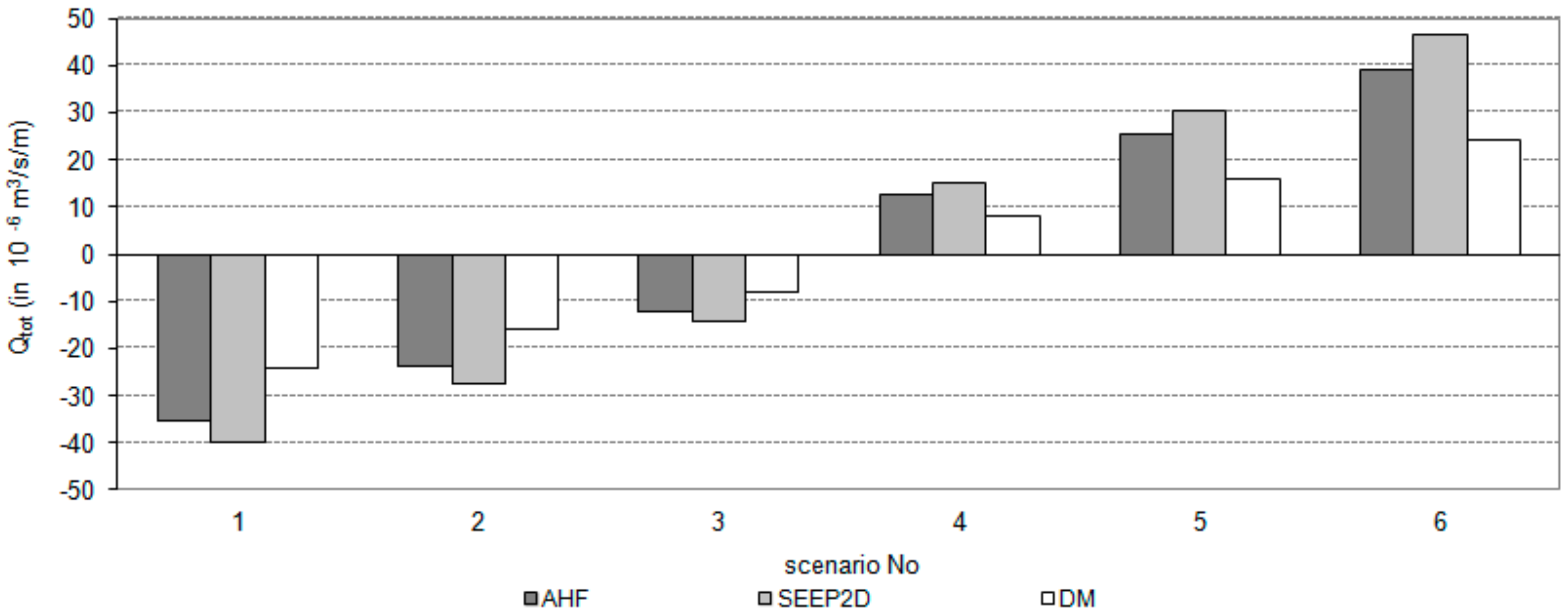
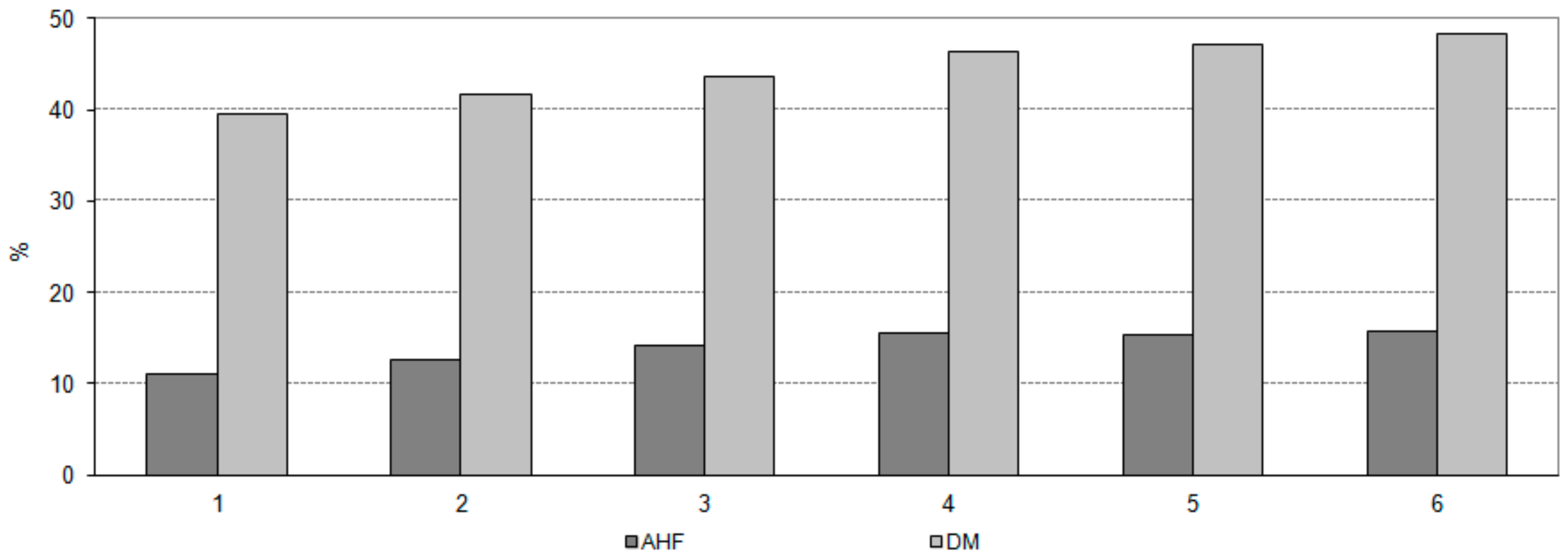
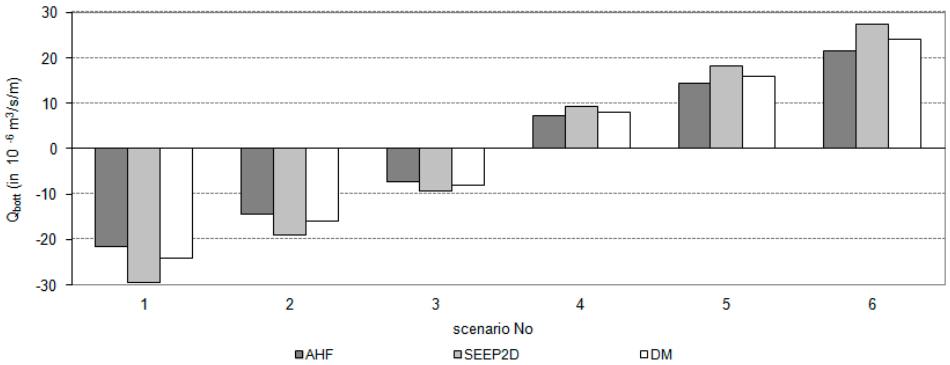
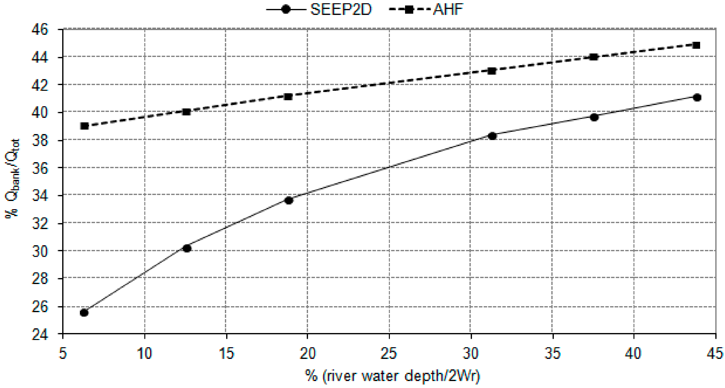
• The AHF model errors (estimated as a difference in total flow Q_tot calculated with the AHF and SEEP2D models) depend on the “depth to width” ratio of water in the riverbed, and on the exchange flow direction-drainage or infiltration to/from the riverbed. They are in a, range of 11 to 16%, and are significantly lower compared to the DM model based on Equation (1) in which the errors are in a range of 40 to 48%.
• A limitation of the AHF model applicability is its geometry—a rectangular-shaped riverbed cross-section followed by the same shape of the sediment layer under its bottom and alongside its bank. Overestimation of Q_tot (AHF) over Q_tot (SEEP2D) can be explained by restrictive assumption of horizontal flow in P.3 assumed in the AHF model.
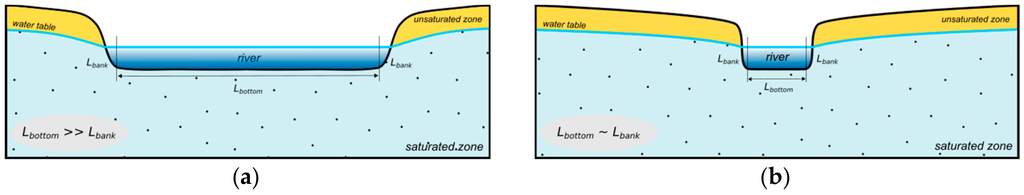
• For small and deep rivers, neglect of flow through the banks (as in the DM model) leads to significant errors in the total flow estimate.

Further work on the development of the AHF model will be aimed at the elimination its most restrictive assumptions.

References

1. Krause, S.; Hannah, D.M.; Fleckenstein, J.H.; Heppell, C.M.; Kaeser, D.; Pickup, R.; Pinay, G.; Robertson, A.L.; Wood, P.J. Inter-disciplinary perspectives on processes in the hyporheic zone. Ecohydrology 2011, 4, 481–499. [Google Scholar] [CrossRef] [Green Version]
2. Boano, F.; Camporeale, C.; Revelli, R.; Ridolfi, L. Sinuosity-driven hyporheic exchange in meandering rivers. Geophys. Res. Lett. 2006, 33. [Google Scholar] [CrossRef]
3. Jekatierynczuk-Rudczyk, E. Strefa hyporeiczna, jej funkcjonowanie i znaczenie. Kosmos 2007, 56, 181–196. [Google Scholar]
4. Zieliński, P.; Jekatierynczuk-Rudczyk, E. Dissolved organic matter transformation in the hyporheic zone of a small lowland river. Oceanol. Hydrobiol. Stud. 2010, 39, 97–103. [Google Scholar] [CrossRef]
5. Boano, F.; Harvey, J.W.; Marion, A.; Packman, A.I.; Revelli, R.; Ridolfi, L.; Wörman, A. Hyporheic flow and transport processes: Mechanisms, models, and biogeochemical implications. Rev. Geophys. 2014, 52, 603–679. [Google Scholar] [CrossRef]
6. Harvey, J.; Gooseff, M. River corridor science: Hydrologic exchange and ecological consequences from bedforms to basins. Water Resour. Res. 2015, 51, 6893–6922. [Google Scholar] [CrossRef] [Green Version]
7. Ward, A.S. The evolution and state of interdisciplinary hyporheic research. Wiley Interdiscip. Rev. Water 2016, 3, 83–103. [Google Scholar] [CrossRef]
8. Peralta-Maraver, I.; Reiss, J.; Robertson, A.L. Interplay of hydrology, community ecology and pollutant attenuation in the hyporheic zone. Sci. Total Environ. 2018, 610–611, 267–275. [Google Scholar] [CrossRef] [Green Version]
9. Schmadel, N.M.; Ward, A.S.; Wondzell, S.M. Hydrologic controls on hyporheic exchange in a headwater mountain stream. Water Resour. Res. 2017, 53, 6260–6278. [Google Scholar] [CrossRef]
10. Hendriks, D.M.D.; Okruszko, T.; Acreman, M.; Grygoruk, M.; Duel, H.; Buijse, T.; Schutten, J.; Mirosław-Świątek, D.; Henriksen, H.J.; Sanches-Navarro, R.; et al. Policy Discussion Paper “Bringing groundwater to the surface” | REFORM. D7.7 Policy Discuss. Pap. No. 2, Reform Proj. 2015. Available online: https://www.reformrivers.eu/policy-discussion-paper-bringing-groundwater-surface (accessed on 6 May 2020).
11. Trauth, N.; Schmidt, C.; Maier, U.; Vieweg, M.; Fleckenstein, J.H. Coupled 3-D stream flow and hyporheic flow model under varying stream and ambient groundwater flow conditions in a pool-riffle system. Water Resour. Res. 2013, 49, 5834–5850. [Google Scholar] [CrossRef]
12. Siergieiev, D.; Ehlert, L.; Reimann, T.; Lundberg, A.; Liedl, R. Modelling hyporheic processes for regulated rivers under transient hydrological and hydrogeological conditions. Hydrol. Earth Syst. Sci. 2015, 19, 329–340. [Google Scholar] [CrossRef] [Green Version]
13. Brunner, P.; Therrien, R.; Renard, P.; Simmons, C.T.; Franssen, H.J.H. Advances in understanding river-groundwater interactions. Rev. Geophys. 2017, 55, 818–854. [Google Scholar] [CrossRef]
14. Sophocleous, M. Interactions between groundwater and surface water: The state of the science. Hydrogeol. J. 2002, 10, 52–67. [Google Scholar] [CrossRef]
15. Grodzka-Łukaszewska, M.; Nawalany, M.; Zijl, W. A Velocity-Oriented Approach for Modflow. Transp. Porous Media 2017, 119, 373–390. [Google Scholar] [CrossRef] [Green Version]
16. Shen, X.; Lampert, D.; Ogle, S.; Reible, D. A software tool for simulating contaminant transport and remedial effectiveness in sediment environments. Environ. Model. Softw. 2018, 109, 104–113. [Google Scholar] [CrossRef]
17. Rushton, K.R.; Tomlinson, L.M. Possible mechanisms for leakage between aquifers and rivers. J. Hydrol. 1979, 40, 49–65. [Google Scholar] [CrossRef]
18. Rushton, K.R.; Rathod, K.S. Horizontal and vertical components of flow deduced from groundwater heads. J. Hydrol. 1985, 79, 261–278. [Google Scholar] [CrossRef]
19. Nawalany, M.; Grodzka-Łukaszewska, M.; Sinicyn, G. Consistency of water balances of surface waters and groundwater (in Polish). Monogr. Water Manag. Comm. Pol. Acad. Sci. 2014, 1, 237–246. [Google Scholar]
20. Carslaw, H.S.; Jaeger, J.C. Conduction of Heat in Solids (Paperback); Oxford University Press: Oxford, UK, 1959; pp. 353–387. [Google Scholar]
21. Harr, M.E. Groundwater and Seepage; American Association for the Advancement of Science (AAAS): Washington, DC, USA, 1963. [Google Scholar] [CrossRef]
22. Polubarinova-Koch, P.I. Theory of Ground Water Movement; Princeton University Press: Princeton, NJ, USA, 1962. [Google Scholar] [CrossRef]
23. Polubarinova-Koch, P.I. Theory of the Motion of Ground Water (in Russian); Nauka: Moscow, Russian, 1977. [Google Scholar]
24. Paniconi, C.; Putti, M. Physically based modeling in catchment hydrology at 50: Survey and outlook. Water Resour. Res. 2015, 51, 7090–7129. [Google Scholar] [CrossRef] [Green Version]
25. Cousquer, Y.; Pryet, A.; Flipo, N.; Delbart, C.; Dupuy, A. Estimating River Conductance from Prior Information to Improve Surface-Subsurface Model Calibration. Groundwater 2017, 55, 408–418. [Google Scholar] [CrossRef]
26. Antontsev, S.N.; Díaz, J.I. On the coupling between channel level and surface ground-water flows. Pure Appl. Geophys. 2008, 165, 1511–1530. [Google Scholar] [CrossRef]
27. Nawalany, M. Mathematical Modeling of River-Aquifer Interactions, Report SR; HR Wallingford: Wallingford, UK, 1993. [Google Scholar]
28. Nawalany, M. Two- and three-dimensional models of groundwater flow. Phys. Appl. 1999. [Google Scholar]
29. Saeedpanah, I.; Golmohamadi Azar, R. New Analytical Expressions for Two-Dimensional Aquifer Adjoining with Streams of Varying Water Level. Water Resour. Manag. 2017, 31, 403–424. [Google Scholar] [CrossRef]
30. Nawalany, M. The Study of Groundwater with the Use of Dynamic System Theory; Publishing Office of Warsaw University of Technology: Warsaw, Poland, 1984. [Google Scholar]
31. Ebel, B.A.; Mirus, B.B.; Heppner, C.S.; VanderKwaak, J.E.; Loague, K. First-order exchange coefficient coupling for simulating surface water-groundwater interactions: Parameter sensitivity and consistency with a physics-based approach. Hydrol. Process. 2009, 23, 1949–1959. [Google Scholar] [CrossRef]
32. Bansal, R.K.; Lande, C.K.; Warke, A. Unsteady groundwater flow over sloping beds: Analytical quantification of stream-aquifer interaction in presence of thin vertical clogging layer. J. Hydrol. Eng. 2016, 21. [Google Scholar] [CrossRef]
33. Jones, N.L. SEEP2D Primer, Environmental Modeling Research Laboratory; Brigham Young University: Provo, UT, USA, 1999. [Google Scholar]
34. Van Genuchten, M.T. A Closed-form Equation for Predicting the Hydraulic Conductivity of Unsaturated Soils. Soil Sci. Soc. Am. J. 1980, 44, 892–898. [Google Scholar] [CrossRef] [Green Version]
Figure 1. Cross section through different shapes of riverbed: (a) Lbott >> Lbank; and (b) Lbott ≈ Lbank.
Water 12 01792 g001
Figure 2. River–aquifer system of the Upper Biebrza River in Poland and outline of the exemplary system geometry used in the AHF and SEEP2D models.
Water 12 01792 g002
Figure 3. Flow subdomains: P.1 and P.2, in aquifer under river sediments; P.3, river sediments right/left of the river bank; P.4, river sediments under river bottom; (y, z), general system of coordinates.
Water 12 01792 g003
Figure 4. Convergence of finite series Q b o t t ( N ) for six scenarios (Φ*Hr).
Water 12 01792 g004
Figure 5. Specific discharge fields and hydraulic head distribution in the river–aquifer system calculated for H r = 28.5 m and Φ * = 27.0 m with (a) AHF and (b) SEEP2D models (both with the assumption of no flow between subregions P.3–P.4 and P.1–P.3).
Water 12 01792 g005
Figure 6. River recharge/discharge by groundwater seepage for different scenarios and models. Negative values of the river seepage indicate that the river is of water-gaining type; positive values occur when the river is of water-losing-type.
Water 12 01792 g006
Figure 7. Errors of river recharge calculated with the AHF analytical model and estimated with the Darcy’s law model (DM) related to the values calculated by the SEEP2D model.
Water 12 01792 g007
Figure 8. River bottom seepage for different scenarios and models.
Water 12 01792 g008
Figure 9. SEEP2D calculated free groundwater table, piezometric head contours, and flow lines for (a) Hr = 28,5 m and Φ* = 27 m and (b) Hr = 25,5 m and Φ* = 27 m.
Water 12 01792 g009
Figure 10. Two sided Qbank seepage contribution to total river flow Qtot (calculated with the SEEP2D and AHF models) as a function of the ratio of water depth (Hr–Da–ds) to river width (2Wr).
Water 12 01792 g010