1. Introduction
The flow in prismatic open channels as a civil engineering specialty has been studied for over 100 years via laboratory experiments, theoretical one-dimensional analysis, as well as with numerical modeling. The flow may be characterized as a gradually varied (GVF) or a rapidly varied (RVF) flow if changes of flow depth are gradual over a significant length or abrupt over a short length of the channel respectively. A characteristic dimensionless parameter describing the type of flow is the Froude number, that expresses the ratio of inertia over the gravity forces, u being the average, over a cross section velocity; g is the gravitational acceleration and D is the hydraulic depth, i.e., the depth of the equivalent orthogonal channel with bottom width equal to the width of free surface of the prismatic channel. When inertia forces are dominant, Fr > 1 and the flow is called supercritical, otherwise when Fr < 1, the flow is named subcritical. Critical flow (Fr = 1) may occur, but it is quite unstable, oscillating between a subcritical and a supercritical state. A special case of a RVF is the hydraulic jump, which is formed in an open channel when supercritical flow turns into subcritical, resulting in an abrupt rise of the free surface, formation of a surface roller and high energy dissipation locally. The hydraulic jump in civil engineering applications can be used as an energy dissipation mechanism, for mixing purposes as well as for the aeration of the flow.
Hydraulic jumps appear usually in stilling basins for energy dissipation of spillways when required. The sequent (subcritical) depth, the length (distance between subcritical and supercritical flow) and the location where the jump occurs are important parameters for the safe design of such structures. Among the experiments performed to determine these parameters are the pioneering works [
1,
2], where the one-dimensional momentum equation was derived relating the sequent depth ratio to the upstream Froude number. Moreover, in more recent experiments on hydraulic jumps [
3,
4,
5,
6,
7], basic flow variables have been determined such as the sequent depth ratio, the length of the jump and the geometry of the surface roller.
The one-dimensional depth-averaged equations of mass conservation (continuity) and momentum (Navier–Stokes), describing the unsteady, rapidly varied open channel flow with non-hydrostatic pressure distribution, form a two-equation system named the Boussinesq equations. Assuming parallel flow and hydrostatics over the depth pressure distribution, the simplified system is called the Saint Venant (shallow water) equation. In both systems of equations the variables are the depth of flow and the average over depth velocity. A hydraulic jump can be modeled using the Boussinesq equations, which is the main objective of this work. So far, the shallow water Saint Venant equations have been used in several investigations for the numerical simulation of the classical hydraulic jump. For example, the finite element method was used [
8] to solve the Saint Venant equations up to the point that steady state was reached. The assumption of hydrostatic pressure distribution employed is not valid in the region of the hydraulic jump, because the substantial curvature of the streamlines results in vertical accelerations that cannot be neglected. Moreover, the energy losses were neglected (weak hydraulic jump), making questionable the validity of simulation results for practical purposes. An attempt was made [
9], to combine the knowledge regarding vorticity generation in a hydraulic jump, using the Navier–Stokes and shallow water equations. The Saint Venant equations were also modified [
10], including terms related to turbulent shear stress and non-uniform velocity distribution, applying a depth-averaged approach. The equations were solved by the finite element method for the location and the profile of a hydraulic jump with upstream Froude numbers in the range 2 to 7. An effort to simulate the classical hydraulic jump using the shallow water equations and solve them using the MacCormack numerical scheme [
11], produced results that compare well with the theoretical ones. The finite volume method [
12] has been used to solve the governing shallow water equations. This model was applied to a hydraulic jump, and the numerical results are in agreement with experiments.
The numerical solution of Navier–Stokes equations has been widely used in modeling of the hydraulic jump. The use of the Reynolds-Averaged Navier–Stokes (RANS) approach and the k-ε turbulence closure model [
13], was applied to study the turbulence characteristics of the hydraulic jump, which had to be adapted to flow cases of a moving free surface by means of the partially explicit approach. The study includes both free and forced hydraulic jumps with Froude numbers in the range from 2.1 to 7.6. Comparison of the numerical predictions with velocity measurements using one-dimensional Laser Doppler Anemometry, showed that the results qualitatively compare well, regarding the mean velocity and turbulence intensity in the flow direction. RANS equations were solved using a turbulence closure k-ε model [
14], to study the hydraulic jump in a straight horizontal channel with Froude numbers 2.0 and 4.0. The mixed Eulerian-Lagrangian method for the calculation of the free surface of the flow is utilized to overcome the problem posed by a moving free boundary. A detailed study of the internal and external characteristics of a hydraulic jump was made and compared to experiments where possible. The surface roller and recirculation zone are found to play a dominant role in turbulence generation and dissipation. The study of free and submerged hydraulic jumps in a rectangular open channel downstream a sluice gate [
15] has also been considered. Air-water two-phase flows are considered in the numerical simulations using RANS and turbulence closure k-ε modeling [
15], and compared to velocity measurements made using Acoustic Doppler and Particle Image Velocimetry. The numerical results concerning water depths, the hydraulic jump length and the velocity profiles compare well with laboratory measurements. A three-dimensional model was implemented [
16], using OpenFOAM software to analyze a hydraulic jump with upstream Froude number 6.1 in a horizontal, smooth, rectangular open channel. RANS equations were solved using three turbulence closure models, namely the Standard k-ε, the Re-Normalization Group (RNG) k-ε, and the Shear Stress Transport (SST) k-ω model. Direct Numerical Simulation (DNS) was used [
17], in a hydraulic jump with Froude number equal 2.0, using the volume of fluid method for tracking the free surface. Results have been produced regarding the mean velocity field, Reynolds stresses, turbulence production and dissipation, velocity spectra and air entrainment concentration. Finally the two recent works [
18,
19] present a very thorough investigation on datasets for numerical modeling assessment of the hydraulic jump.
In summary, the shallow water one-dimensional equations are capable of modeling only some characteristics of a transient hydraulic jump, while RANS combined with turbulence closure models or DNS can capture the turbulent structure of a steady hydraulic jump more accurately. Implementation of such algorithms though is limited by the Reynolds number of the flow that usually exceeds 106. Moreover, the computational cost of such models is very high, because the computational time if a decent computing machine is very long. For practical, mainly civil engineering applications, shallow water modeling is much simpler to use, while the results can be acceptable. In the present work, we will show that one-dimensional modeling of a hydraulic jump is improved using the more accurate, unsteady, one-dimensional Boussinesq equations. They are solved numerically using the MacCormack and the Dissipative two-four finite difference schemes. The practicality of such a model used in applications like the design of stilling basins, has led us to choose this model for analysis. The maximum error of the flow depth is used as an iterative parameter, for achieving the steady state solution for the free surface profile and the location of a hydraulic jump, in a horizontal rectangular open channel for a wide range of Froude numbers. To apply the Boussinesq model at the downstream boundary node, the method of specified intervals was used for the evaluation of the unknown flow variables. The results are compared to experiments performed at the Laboratory of Applied Hydraulics, School of Civil Engineering, National Technical University of Athens, Greece, showing that such numerical schemes can accurately simulate the classical hydraulic jump.
2. Governing Equations
The equations modeling unsteady one-dimensional rapidly varied flows are the Boussinesq equations [
20]. These include additional terms for the non-hydrostatic pressure distribution due to curved streamlines. The basic assumptions made are: (1) the vertical velocity varies from zero at the channel bottom to its maximum value at the free surface, (2) the velocity in the main flow direction is uniformly distributed over the depth, (3) the velocity in the lateral direction is zero, (4) the fluid is incompressible, (5) the channel is prismatic of a rectangular cross section with rigid bottom and sides, (6) the longitudinal bottom slope is small, and (7) the formulas regarding energy friction slope for steady flow can be used for the unsteady flow as well. The one-dimensional Boussinesq equations for mass and momentum conservation are written in vector form as:
where:
x is the longitudinal distance along the channel bottom as shown in
Figure 1, t is the time, h = h(x,t) and u = u(x,t) are the unknown flow depth and mean velocity components in the main flow direction respectively, S
f is the energy grade line slope, S
o is the longitudinal bottom slope and g is the gravitational acceleration. E = E(x,t) is the Boussinesq term, which makes the difference if compared to the Saint Venant equations where the pressure distribution is assumed to be hydrostatic. The energy grade slope can be computed using the Manning formula in SI, u = (R
2/3S
1/2)/n, where u is the mean over the wetted cross-section velocity, R is the hydraulic radius (cross sectional area over the wetted perimeter ratio), S = S
f the energy grade slope and n the Manning friction coefficient as S
f =
u
2/R
4/3. Alternatively, the Darcy–Weisbach formula could be used for computing S
f, but we used the Manning formula in order to simplify calculations since the friction coefficient is kept constant for every step and the results are not affected.
3. Numerical Schemes
The classical hydraulic jump Boussinesq equations cannot be solved analytically, therefore a numerical method has to be implemented. In this work, the MacCormack [
21] and the Dissipative two-four [
22] finite difference schemes have been employed for the solution of the flow equations with the appropriate initial and boundary conditions. The first scheme is second order accurate both in space and time, and the second one is fourth order accurate in space and second order in time, allowing for proper simulation of the Boussinesq terms. The developed algorithm iterates until the change of the flow depth between two successive iterations is less than a fixed convergence value. Then the jump forms a part of the steady state solution.
A sketch of the jump with the computational grid is shown in
Figure 1. The hydraulic jump is formed combining the use of a sluice gate upstream with a weir downstream. The origin of the spatial coordinate (x = 0) is set at the sluice gate location, while x is the longitudinal distance along the channel bottom measured from the origin. The distance between the sluice gate and the weir is L (equal to 5.20 m, the region of interest where the computational solution is sought), and it is discretized by a total number of n nodes including the boundary nodes, thus creating a uniform grid of points at distance Δx = L/(n−1) in between. The index i denotes a spatial node, while the upstream and downstream boundaries correspond to nodes i = 1 and i = n with flow depths denoted as h
up and h
do respectively. A brief presentation of the numerical schemes for the discretization of Equation (1) follows.
3.1. MacCormack Scheme
This scheme is a two-step algorithm. For the spatial derivatives of Equation (1) forward finite differences are used in the predictor step and backward finite differences in the corrector step including in the computational stencil two spatial nodes in the predictor step, the nodes i + 1, i and in the corrector step the nodes i and i − 1 as follows:
The flow variables at the next iteration level k+1, and grid point i, are given by:
where λ = Δt/Δx, Δt being the time interval and the superscripts k and k + 1 refer to the two successive levels of iteration. All variables with a single asterisk (*) refer to those computed at the predictor step where all variables with double asterisk (**) refer to those computed at the corrector step. The Boussinesq terms are neglected in this scheme.
3.2. Dissipative Two-Four Scheme
The Dissipative two-four scheme consists of a predictor and a corrector step, again for the spatial derivatives of Equation (1) forward finite differences are used in the predictor step and backward finite differences having in the corrector step, as including in the computational stencil, three spatial nodes in the predictor step, the nodes i + 2, i + 1 and i and in the corrector step the nodes i, i − 1 and i − 2:
The vector
at the next iteration level k + 1 and grid point i, is given by:
Regarding Boussinesq terms, the second order derivative is approximated using a three point central finite difference in both steps, while for the first order derivative , forward finite difference is used in the predictor step, and a backward finite difference in the corrector step. The partial derivative in the Boussinesq terms is ignored, since it is zero at steady state. Regarding the code implementation, Equations (4)–(9), have to be written in non-vector form.
Due to computational reasons in the case of the Dissipative two-four scheme, the flow equations are discretized using Equations (7) and (8) at the interior nodes, i.e., for i = 4, 5,…, n−2, the Boussinesq terms are either considered or neglected, while at nodes i = 2, 3, n−1, the MacCormack scheme is used for discretizing Equations (4) and (5) and omitting the Boussinesq terms. Apparently, this is allowed since the jump appears far from the boundary nodes, therefore the Boussinesq terms are not significant since the flow is parallel.
3.3. Initial and Boundary Conditions
The appropriate initial and boundary conditions must be set in a well-posed problem. The number of characteristics that enter the computational domain determine the auxiliary conditions to be specified [
23]. The initial condition includes steady, supercritical, gradually varied flow for the entire length of the channel, resulting in two characteristic curves entering the computational domain, thus two flow parameters must be specified at each grid point, the flow depth and the velocity. The depth at each grid point can be computed by numerical integration of the first order ordinary differential equation:
of the steady state gradually varied flow, Fr being the Froude number,
. The upstream depth h
up is known (obtained from the experiments downstream of the sluice gate) and the computation is performed with a Kutta-Merson method, beginning the calculations with the flow depth h
up.
The flow conditions are fixed at the two boundaries of the channel. For a given discharge and settings of the sluice gate upstream and the thin crested weir downstream, the flow depths are known and take constant values hup and hdo at nodes i = 1 and i = n respectively. The mean velocity is known at i = 1 but it has to be computed at end node i = n. Apparently, the flow is assumed to be supercritical at node i = 1 and subcritical at node i = n.
The velocity at the end node i = n will be computed using the method of specified intervals and the positive characteristic equation discretized by finite differences. From
Figure 1, points A and B correspond to nodes n−1 and n respectively at the known time level k, while the positive characteristic through point P with the unknown velocity at the downstream boundary at time level k+1 is indicated. The method of specified intervals is used to compute the velocity, the celerity and the flow depth at point R, which is the intersection of the positive characteristic through point P with the grid line of the known time level k using the following relationships [
24]:
where
is the celerity of a small amplitude wave propagating inside a rectangular open channel in shallow water. The energy grade line slope at point R is estimated from the following Equation:
Then the velocity
at point P can be computed from the following relationship:
3.4. Courant Condition Artificial Viscosity
The variable time step Δt in each iteration is restricted according to the Courant criterion for stability purposes, and it is computed from:
where c
n is the Courant number that must be less than or equal to 0.65 [
24], and Δx is the constant spatial step as shown in
Figure 1.
To dampen the oscillations that occur around the jump region, artificial viscosity has to be added to the numerical schemes. The formulas used are those proposed by [
25].
First the parameter ξ
i at the computational node i is calculated:
Then at the center of segment i + 1/2, between nodes i and i + 1:
Similarity between nodes i − 1 and i:
where k
art is a coefficient adjusting the amount of dissipation.
Finally the flow variables h and u, at iteration level k+1 are modified to the new ones according to the following relationships:
where the variable f stands either for the flow depth or for the velocity. The numerical codes have been implemented in house using Matlab
® computational environment, while the input data for the numerical simulations are the channel geometry, the flow depths h
up, h
do and the flow rate Q.
4. Results
The experiments were performed at the Laboratory of Applied Hydraulics of the School of Civil Engineering at the National Technical University of Athens, Greece, in a 10.50 m long flume with a rectangular cross section 0.248 m wide and 0.50 m deep. The channel has a steel bottom and vertical side walls made of glass. The water supply system consists of a constant head tank, a pipeline and a regulating valve to adjust the flow rate that was measured with a Venturi meter and did not exceed 50 L/s. The flow was controlled by a sluice gate setting the supercritical flow conditions upstream, and a thin crested weir at the end of the channel located 5.20 m downstream from the sluice gate for controlling the tailwater, subcritical flow. The hydraulic jump formed at some location between the sluice gate and the weir, depending upon the upstream, supercritical and tailwater, subcritical depths. The flow depths and free surface profile of the jumps were measured by a point gauge with accuracy ±0.1 mm.
Six experiments were implemented, the flow conditions of which are shown in
Table 1. In the table appear the flow rate q, the supercritical upstream and subcritical downstream depths h
up and h
do respectively, and the Froude number of the flow, Fr, at the toe of the jump from the experimental measurements. The six different jump cases measured, were computed using same conditions (upstream and tailwater depths and the flow rate) and the numerical results are compared to experiments in the following paragraphs.
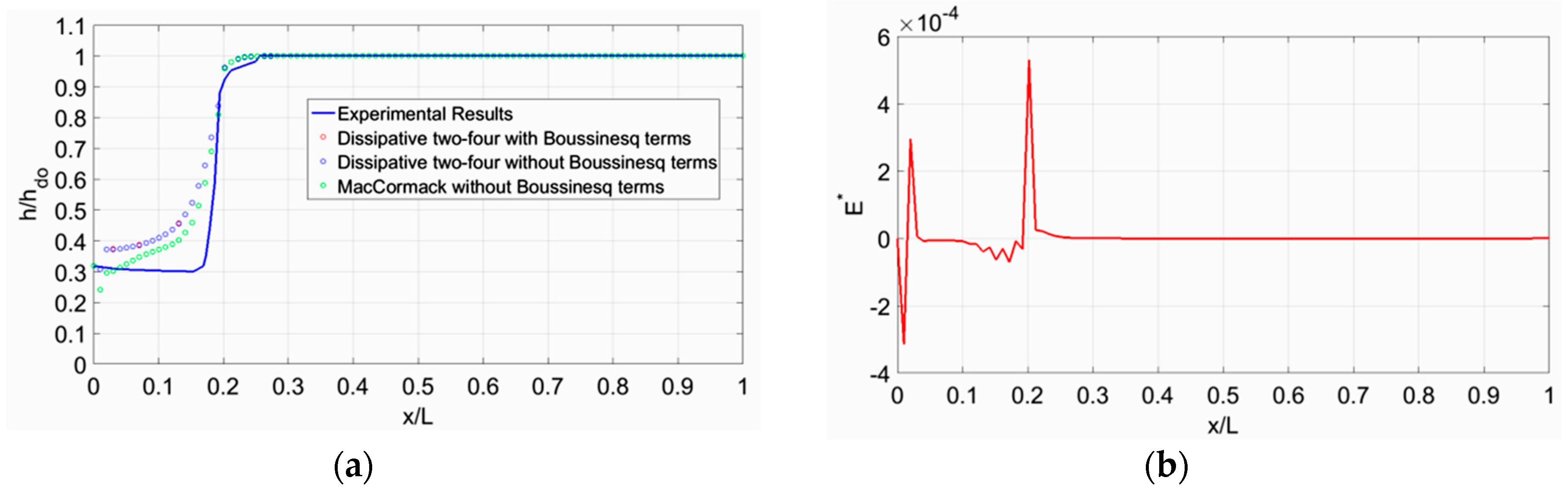
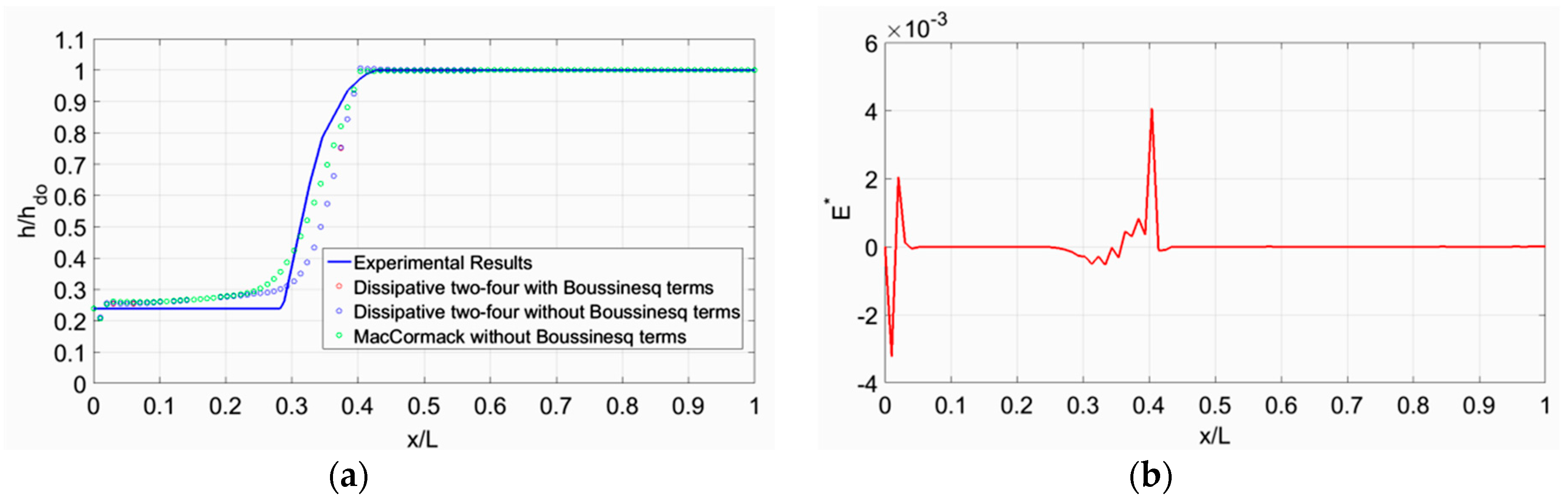
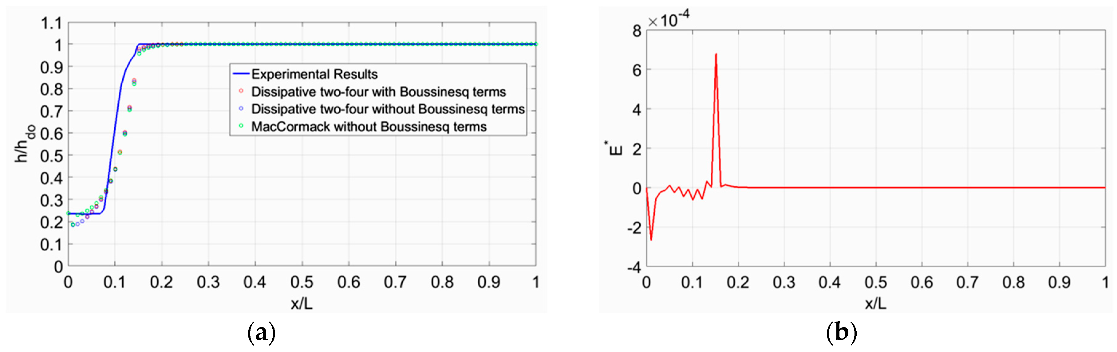
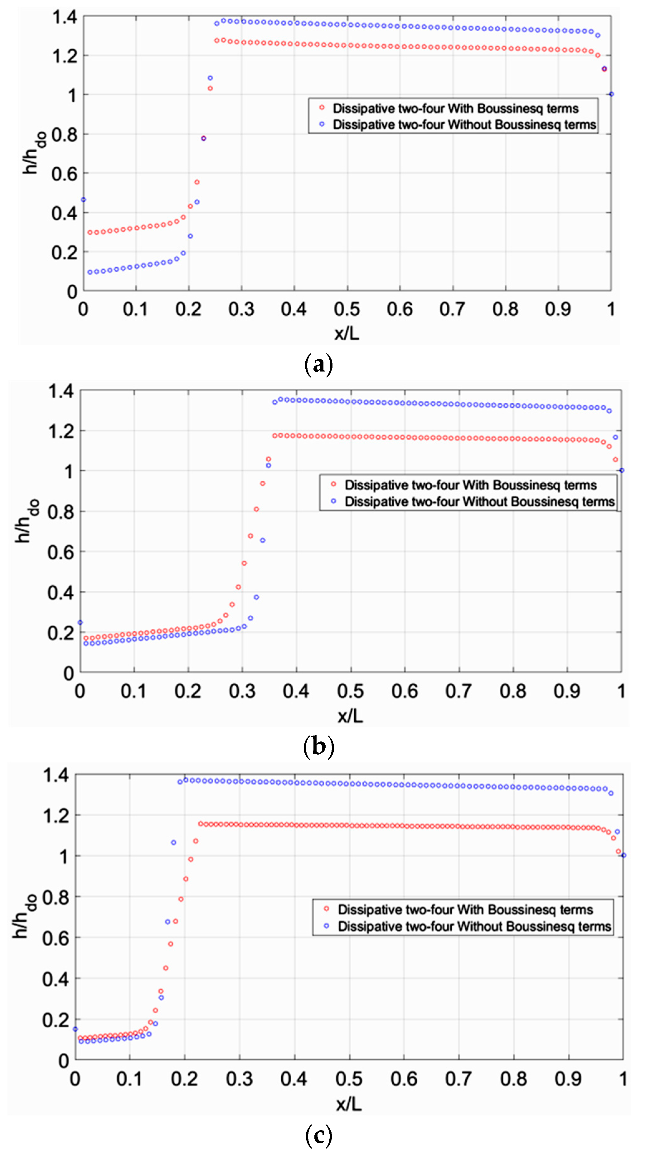
For the numerical modeling of the experiments shown in
Table 1 three discretizing schemes of the Boussinesq equations were used: (i) the Dissipative two-four scheme with the influence of Boussinesq terms, (ii) the Dissipative two-four scheme without the influence of non-hydrostatic pressure distribution terms, and (iii) the MacCormack scheme without Boussinesq terms. The time interval computed from Equation (16) varied in every iteration. Moreover, Equation (22) was applied to dampen the oscillations near the jump. In all test cases 100 spatial nodes were used for discretization (n = 100), resulting in Δx = 0.0525 m with acceptable spatial resolution. All the results regarding the computed dimensionless flow depth h/h
do, alongside the dimensionless longitudinal distance of the channel, x/L, for each test case are shown in
Figure 2a,
Figure 3a,
Figure 4a,
Figure 5a,
Figure 6a and
Figure 7a. The measured and computed flow profiles by the three numerical algorithms are plotted together along the channel, and the significance of the Boussinesq terms (due to non-parallel streamlines) inside the region of the hydraulic jump are depicted sideways in
Figure 2b,
Figure 3b,
Figure 4b,
Figure 5b,
Figure 6b and
Figure 7b. Outside the jump these terms are almost zero (small enough), thus confirming the hydrostatic pressure distribution. From the numerical results, it must be noted that the flow depth increases from the vena contracta downstream of the sluice gate up to the jump, due to energy losses encountered in the governing equations. One may note that in test case 1, the dissipative behavior of the numerical results is probably due to the artificial dissipation added in the numerical scheme. In addition, from the Boussinesq term distribution along the channel, one may note that this term is not zero at the upstream end, therefore we would not expect a smooth transition in free surface from supercritical to subcritical flow. Furthermore, note that the Froude number is quite low and the hydraulic jump is characterized as weak [
26], since 1.7 < Fr < 2.5, which means that it is a non-fully developed jump because of the weak surface roller with low energy loss. From these figures we conclude that the agreement between experiments and computations is satisfactory.
Figure 8a,b exhibit the variation of the dimensionless spatially (over a cross-section) averaged flow velocity in the main flow direction x, u/u
up, where u
up is the average velocity at x = 0, with the dimensionless longitudinal distance, x/L, for all three algorithms for test cases 1 and 6 respectively. It is evident that the MacCormack scheme overestimates the flow velocity at the upstream end of the channel, while the results from the other two methods are almost identical.
Figure 9a,b depict the evolution of convergence criteria of the maximum absolute change in flow depth between two successive iterations, until a steady state is obtained for test case 2 using the Dissipative two-four scheme with Boussinesq terms, and test case 5 using the MacCormack scheme without Boussinesq terms respectively.
Figure 10 and
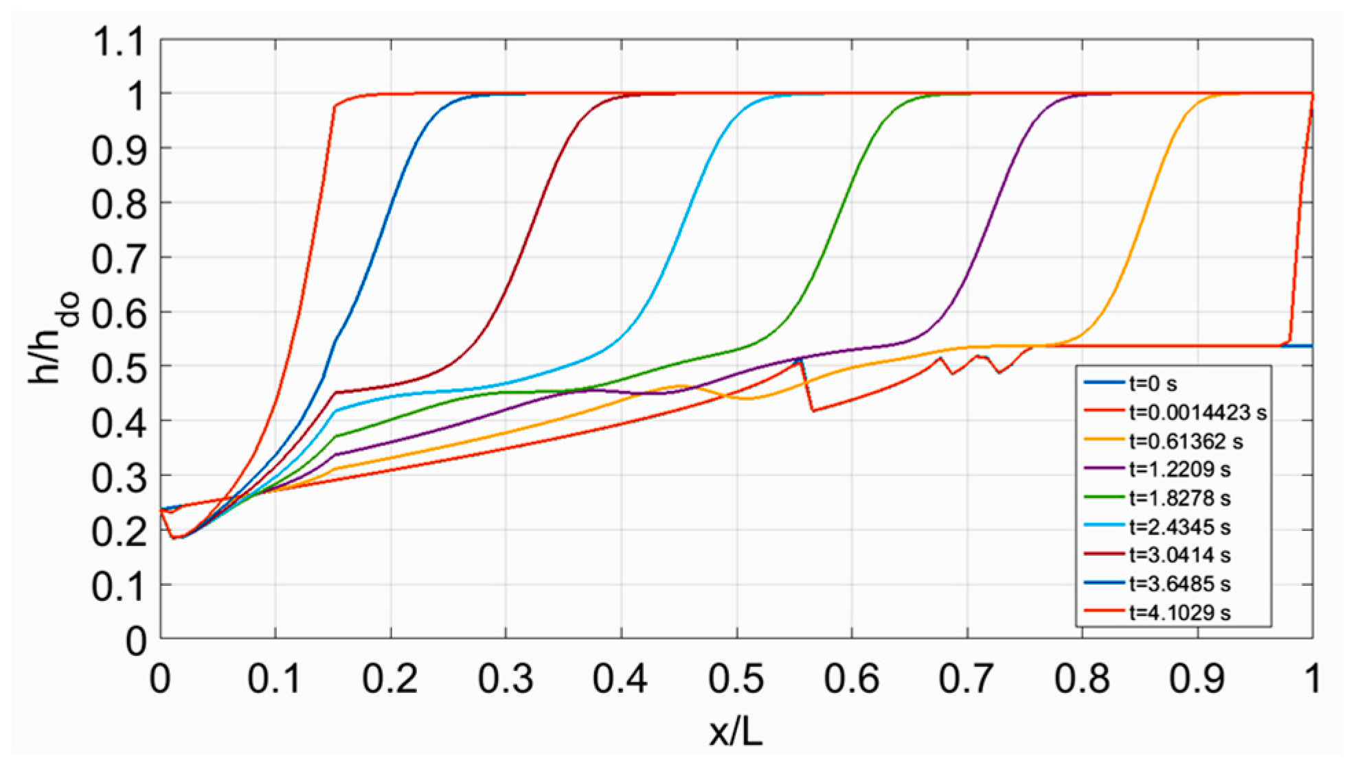
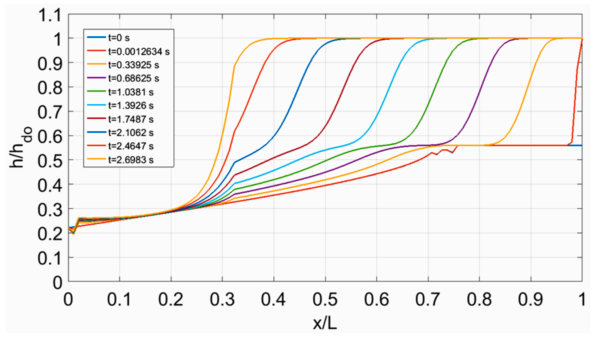
Figure 11 present the temporal evolution in ‘‘computational-pseudo time’’ of the free surface elevation for the Dissipative two-four scheme including the Boussinesq terms for test cases 3 and 4 respectively, both in dimensionless form. Note that the jump moves upstream until it is stabilized. Similar results have been produced for all other test cases.
The specific force of the flow (momentum flux per unit weight) in a channel with rectangular cross section written as
, where b is the width of the rectangular cross section, is conserved across a hydraulic jump, or alternatively, it takes the same value upstream and downstream of the jump. From the numerical results it turns out that the relative error of the specific force between the two end cross-sections of the jump for all test cases and the three numerical schemes applied ranged from 0.62 % to 12.92 %, results that are acceptable for the accurate location of the jump. The number of iterations required to obtain a steady state with accuracy of order 10
−4 m or 5 × 10
−5 m, along with the closure of continuity equation for each test case and all numerical schemes are shown in
Table 2, where the flow rate was computed from the depth and the average velocity over the cross section. It is evident that for all test cases the MacCormack algorithm gave the highest error in mass conservation, if compared to the other algorithms, due to the lower order of spatial accuracy.
An iterative algorithm was implemented for both numerical schemes which converged to the steady state solution, when the maximum value of the difference of the flow depth between two successive iterations was smaller than a threshold value. The sequent depths as well as the location where the jump forms for given flow and boundary conditions, resulted from the steady state solution of the governing equations. The numerical results showed that the magnitude of the Boussinesq terms is greater at the jump regime, whereas outside this it is almost zero, as expected. It was also shown that the Boussinesq terms do not affect practically the location where the jump forms for test cases 1–6, so that their exclusion eases the discretization without significant error. Note that to obtain the results presented in this paper artificial viscosity has been used. A coefficient adjusting the amount of dissipation to reproduce the experimental measurements by a trial and error procedure was set to the value 0.011.
5. Case Studies
For further validation of the numerical results obtained from the six test cases examined, let us present a case study of practical interest. We consider a 100 m long and 2 m wide (narrow channel, depth to width ratio around one) rectangular, horizontal open channel, with Manning roughness coefficient 0.013 and flow rate 7.2 m
3/s. In
Figure 12a–c we present the computed dimensionless flow depth, h/h
do, versus the dimensionless distance x/L, for three Froude numbers at the vena contracta cross-section namely 2, 4 and 6, including or excluding the Boussinesq terms, using a dissipation parameter equal to 0.011. In
Figure 12d we demonstrate the temporal evolution of the jump until it is stabilized, for Froude number equal to 4. In all three cases one may notice the formation of H3 and H2 types of free surface curves upstream and downstream of the jump respectively, due to energy loss. From
Figure 12b,c it is evident that the hydraulic jump is much longer when computed using Boussinesq terms.
Let us now examine the influence of the channel width on the length of the hydraulic jump, L
j. We consider a 100 m long channel and 5 m wide (wide section, depth to width ratio smaller than one) with orthogonal cross section conveying 10 m
3/s, with same dissipation factor equal to 0.011. In
Figure 13a–c the computed dimensionless flow depth, h/h
do, is plotted versus the dimensionless distance x/L, for three Froude numbers at the vena contracta namely 2, 4 and 6, with or without the Boussinesq terms incorporated. The flow depth at x/L = 0 is the boundary condition, and it is the same with and without Boussinesq terms, as indicated in
Figure 12 and
Figure 13. Near the supercritical boundary the depth deviates from that at x/L = 0, with deviation being greater when Boussinesq terms are not included. This is probably due to numerical instability from the boundary condition, also shown clearly in
Figure 2b,
Figure 3b,
Figure 4b,
Figure 5b,
Figure 6b and
Figure 7b, where Boussinesq terms are plotted vs x/L. The non-Boussinesq terms showed greater instability because the depth near the supercritical boundary deviates more than that with Boussinesq terms.
The length of the hydraulic jump computed with Boussinesq terms, is still greater than that computed without incorporating Boussinesq terms, but the difference is not as sound as it was in the previous example. In
Table 3 and
Table 4 we present the length of the computed hydraulic jump and compare it to that from experiments [
27] (p. 14). The results in the 5 m wide channel with or without the Boussinesq terms are in satisfactory agreement with measurements in orthogonal channels, if compared to the results of the 2 m wide channel. The noticeable differences between the flow profiles in
Figure 12 and
Figure 13 are probably due to the non-hydrostatic pressure distribution encountered in Boussinesq terms. The difference is sound when the hydraulic jump is “weak” for low Froude numbers, where the transition from supercritical to subcritical flow is not as vigorous as for greater Froude numbers. Therefore there is a smoother free surface elevation when Boussinesq terms are included, resulting in longer jump lengths.
From
Table 3, it is obvious that comparing the numerical results with experiments, exclusion of Boussinesq terms leads to more accurate results concerning the length of the jump. Alternatively, from
Table 4 the opposite is true. Apparently, the flow in a “wide” orthogonal open channel is not affected from the side walls while in a “narrow” channel, it is. Therefore, the one-dimensional shallow water equations that are improved with Boussinesq terms can predict the characteristics of a hydraulic jump accurately, if the channel is wide if compared to the flow depth.
6. Conclusions
The one-dimensional Boussinesq equations have been solved numerically using the MacCormack as well as the Dissipative two-four finite difference schemes, for the simulation of hydraulic jump formation in a horizontal rectangular open channel and for upstream Froude numbers Fr in the range 2.44 to 5.38. The governing equations have been enriched with additional terms if compared to the Saint Venant equations, to account for the non-hydrostatic pressure distribution in the regime of rapidly varied flow. Terms related to the energy loss and the gravity forces have been also included. The initial condition was a steady supercritical gradually varied flow along the whole length of the channel modeled. The upstream and downstream boundary conditions regarding the flow depth remained constant during the iteration process, and equal to the values measured in experiments. The method of specified intervals was used for the calculation of the velocity at the downstream end, assuming that the positive characteristic through a point does not intersect with already established grid points. Variable time step was used in every iteration according to the CFL (Courant-Friedrichs-Lewy) stability criterion, along with artificial viscosity for smoothing of the oscillations occurring in the jump. The computational results compare well with experiments since the specific force was computed from the depth and mean velocity at both ends of the hydraulic jump with acceptable tolerance, and the mass conservation equation was verified for all numerical schemes and all test cases.
From such a model one can determine the sequent depth ratio as well as the length of the jump, results that are useful in the design of stilling basins (geometrical properties). Given a stilling basin with a known inflow Froude number and flow depth, the engineer must decide the end sill dimensions and the basin length, so that the hydraulic jump is contained in the stilling basin. Finally, from comparison of the numerical results and experiments, it can be concluded that the aforementioned numerical modeling schemes can predict the basic features of the classical hydraulic jump with acceptable accuracy.


