Medium-Term Rainfall Forecasts Using Artificial Neural Networks with Monte-Carlo Cross-Validation and Aggregation for the Han River Basin, Korea

Abstract

In this study, artificial neural network (ANN) models were constructed to predict the rainfall during May and June for the Han River basin, South Korea. This was achieved using the lagged global climate indices and historical rainfall data. Monte-Carlo cross-validation and aggregation (MCCVA) was applied to create an ensemble of forecasts. The input-output patterns were randomly divided into training, validation, and test datasets. This was done 100 times to achieve diverse data splitting. In each data splitting, ANN training was repeated 100 times using randomly assigned initial weight vectors of the network to construct 10,000 prediction ensembles and estimate their prediction uncertainty interval. The optimal ANN model that was used to forecast the monthly rainfall in May had 11 input variables of the lagged climate indices such as the Arctic Oscillation (AO), East Atlantic/Western Russia Pattern (EAWR), Polar/Eurasia Pattern (POL), Quasi-Biennial Oscillation (QBO), Sahel Precipitation Index (SPI), and Western Pacific Index (WP). The ensemble of the rainfall forecasts exhibited the values of the averaged root mean squared error (RMSE) of 27.4, 33.6, and 39.5 mm, and the averaged correlation coefficient (CC) of 0.809, 0.725, and 0.641 for the training, validation, and test sets, respectively. The estimated uncertainty band has covered 58.5% of observed rainfall data with an average band width of 50.0 mm, exhibiting acceptable results. The ANN forecasting model for June has 9 input variables, which differed from May, of the Atlantic Meridional Mode (AMM), East Pacific/North Pacific Oscillation (EPNP), North Atlantic Oscillation (NAO), Scandinavia Pattern (SCAND), Equatorial Eastern Pacific SLP (SLP_EEP), and POL. The averaged RMSE values are 39.5, 46.1, and 62.1 mm, and the averaged CC values are 0.853, 0.771, and 0.683 for the training, validation, and test sets, respectively. The estimated uncertainty band for June rainfall forecasts generally has a coverage of 67.9% with an average band width of 83.0 mm. It can be concluded that the neural network with MCCVA enables us to provide acceptable medium-term rainfall forecasts and define the prediction uncertainty interval.

1. Introduction

Accurate and timely rainfall forecasting is necessary for efficient water resources management, flood protection, and drought risk mitigation [1]. In particular, rainfall forecasting on a monthly or seasonal basis has positive effects on effective water resources allocation, water supply planning, and water demand reduction during a drought period. Medium to long-term rainfall forecasting is an interesting and challenging matter in the fields of meteorology and hydrology.

In recent years, the use of data-driven techniques such as artificial neural networks (ANNs), support vector machines (SVMs), and fuzzy logic systems has increased for developing hydrological and meteorological prediction models. In particular, ANN has been extensively used for rainfall forecasting because it has the ability to capture the complex nonlinear relationship between input and output variables without requiring detailed knowledge of the physical process [2].

The performances of ANN models are highly dependent on the selection of appropriate input variables. Significant efforts are required to determine significant input variables of the model because their effects on output may not often be known a priori. Large scale climate signals can affect the long-term rainfall occurrence in a far-distance region [3,4,5]. Accordingly, many researchers suggested that neural networks have the potential to well produce monthly and seasonal rainfall forecasts using the global climate indices as input parameters in many parts of the world. Abbot and Marohasy [6] used the historical monthly rainfall, atmospheric temperature, and solar data, as well as the lagged climate indices of the Southern Oscillation Index (SOI), Dipole Mode Index (DMI), Pacific Decadal Oscillation (PDO), and El Nino Southern Oscillation (ENSO) to forecast the monthly rainfall for locations in Queensland, Australia. The model was further improved by using forecast values for climate indices in addition to the lagged ones [7], as well as by extending the forecasting lead times by up to nine months [8] and twelve months [9] for locations in the Murray Darling basin, Australia. Mekanki, et al. [1] applied the ANN and multiple regression analysis to forecast the long-term spring rainfall in Victoria in Australia using the lagged ENSO and Indian Ocean Dipole (IOD) as potential predictors. They showed that ANNs are better in finding the pattern and the trend of the observations in comparison to multiple regression models. Kumar et al. [10] used the climate indices of ENSO, the Equatorial Indian Ocean Oscillation (EQUINOO), and Ocean-Land Temperatures Contrasts (OLTC) as predictors to forecast the monthly and seasonal (summer monsoon) rainfall for the state of Orissain in India. Hartmann et al. [11] developed a neural network model to predict the summer rainfall in the Yangtze River basin in China. This was achieved using the climate indices of the SOI, the East Atlantic/Western Russia (EA/WR) pattern, and the Scandinavia (SCA) pattern together with other diverse indices, including the sea surface temperatures, the sea level pressure, and snow data. Yuan et al. [12] predicted the summer rainfall in some parts of the Yellow River basin in China using ANNs. The input variables included the North Atlantic Oscillation (NAO), West Pacific (WP) pattern, Polar Eurasian (POL) pattern, and ENSO (NINO3.4 SSTA). Lee et al. [13] used the lagged climate indices of EA, NAO, PDO, the East Pacific/North Pacific Oscillation (EP/NP), and the Tropical Northern Atlantic Index (TNA) of the ANN input to forecast the late spring-early summer rainfall for the Geum River basin in South Korea. Zahmatkesh and Goharian [14] developed and compared an ANN model and a decision analysis method to forecast the rainfall one month in advance for western Canadian watersheds, using a set of large climate signals with different lag times.

Generally, the forecast model performance is evaluated via cross-validation. Most of the above-mentioned studies used a holdout cross-validation technique in which the learning dataset is divided into two (training and validation) or three (training, validation, and testing) mutually exclusive subsets. Lee et al. [13] used a k-fold cross-validation technique that separates the dataset into k disjoint subsets for similar or nearly similar sizes. This technique trains the model k times with each subset for the validation set as well as the other parts of the training set, and then, the combined errors were evaluated. Appropriate data splitting is important for the cross-validation process because the chosen split can significantly affect the final model performance. An improper data split can lead to high variance in the prediction model performance. The Monte-Carlo cross-validation method (Picard and Cook [15]) can be used to overcome the high variance of the model performance, denoted as a repeated random subsampling or random splitting. Shao [16] has proven that the Monte-Carlo cross-validation method is asymptotically consistent, and it can increase the probability of selecting the best performing model. Xu et al. [17] evaluated Monte-Carlo cross-validation for selecting a model and estimating its prediction ability. Barrow and Crone [18] proposed the Monte-Carlo cross-validation and aggregation (MCCVA) method for combining neural network forecasts, which combines bootstrapping and cross-validation in a single approach through the repeated random splitting of the original learning data into mutually disjoint datasets for training and validation. However, the Monte-Carlo cross-validation method does not significantly focus on the ANN-based medium to long-term rainfall forecasting. Our study uses the MCCVA method to generate an ensemble of forecasts, and it evaluates the performance of the rainfall forecasting model.

The objective of this study is to develop practical ANN models using MCCVA to forecast the rainfall for the Han River basin in South Korea during May and June. This time period was selected because this is when agricultural water demand abruptly increases and severe droughts in recent years have occurred during both months. The monthly global climate indices and past rainfall data with different lag times are determined as the predictors of the ANN models. The MCCVA method is used for random subsampling to split the entire dataset, create diverse networks, and evaluate the general performance of the resulting ensemble of rainfall forecasts. In addition, the output uncertainty arising from the variability of the network parameters is assessed by constructing the prediction interval.

2. Data and Methods

2.1. Data

The study area of the Han River basin (Figure 1) is located in the central region of the Korean Peninsula. A substantial proportion of the basin, 86.1% of the total area of 34,428 km², is located in South Korea, and the remainder is located in North Korea.

The South Korea’s Ministry of the Environment provides the area-averaged rainfall data along the basin scale. The data was calculated by using the Thiessen method so that the rainfall was measured at gauging points within and around the basin. The historical monthly area-averaged rainfall data for the Han River basin has been recorded since 1966, and it was obtained from the Water Resources Information System [19].

The choice of appropriate input variables is crucial in prediction modeling. Generally, the selection of input variables is based on a priori knowledge of causal variables [20]. Kim et al. [21] investigated the relationships between the large-scale atmospheric teleconnection and the warm season hydro-climatology in the Han River basin. They found that the East Atlantic/Western Russia Pattern (EAWR) and East Atlantic Pattern (EA) patterns show a significant relationship with the regional precipitation and streamflow. Kim et al. [22] analyzed the past and future extreme weather events and the associated flow regime of the Han River basin using a variety of local extreme climate indices. However, a priori knowledge to choose the large-scale climate indices affecting the monthly and seasonal rainfall is not sufficient to be used for the study area, particularly for the target months (May and June) for this study. There may exist a large number of potential inputs that affect the rainfall occurrence in May and June for the target forecast months. Finding the most significant input variables using trial-and-error can be time-consuming; thus, this study uses a cross-correlation analysis to determine the candidate input variables that could be potentially related to a target rainfall occurrence.

Large-scale climate indices have been widely used for seasonal predictions because these indices compactly can express the regional variabilities of the atmosphere and the surface of the land and ocean [23]. These climate indices are updated on a monthly basis by the climate prediction center (CPC) under the National Oceanic and Atmospheric Administration (NOAA). Users can easily obtain information on the various climate indices from the website [24]. Many climate indices have been provided from 1950 to the present. In this study, the potential climate indices data for 54 years from 1965 to 2018 were collected and are summarized in

Table 1. List of climate indices used in the correlation analysis.

Abbreviation	Full name	Description
AAO	Antarctic Oscillation	The first leading mode from the Empirical Orthogonal Function (EOF) analysis of the monthly mean height anomalies at 700-hPa
AMM	Atlantic Meridional Mode	A climate mode associated with the cross-equatorial meridional gradient of the sea surface temperature anomaly (SSTA) in the tropical Atlantic
AMO	Atlantic Multidecadal Oscillation	A coherent mode of natural variability based upon the average anomalies of the sea surface temperatures (SST) in the North Atlantic basin, which is typically over 0–80° N
AO	Arctic Oscillation	The first leading mode from the Empirical Orthogonal Function (EOF) analysis of the monthly mean height anomalies at 1000-hPa
BEST	Bivariate ENSO Time series	Bivariate ENSO calculated by combining a standardized SOI and a standardized Niño 3.4 SST time series
CAR	Caribbean SST Index	The time series of the SST anomalies averaged over the Caribbean
EA	East Atlantic Pattern	The second prominent mode of the low-frequency variability over the North Atlantic, and it appears as a leading mode for all months
EAWR	East Atlantic/Western Russia Pattern	One of three prominent teleconnection patterns, which affects Eurasia throughout the year
EPNP	East Pacific/North Pacific Oscillation	A spring–summer–fall pattern with three main anomaly centers
GML	Global Mean Land Ocean Temperature Index	Anomaly index from the NASA Goddard Institute for Space Studies (GISS)
MEI.v2	Multivariate ENSO Index version 2	The multivariate ENSO index (MEI V2) time series is bimonthly so the Jan value represents the Dec-Jan value and it is centered between the months
NAO	North Atlantic Oscillation	One of the most prominent teleconnection patterns for all seasons
NINO1+2	Extreme Eastern Tropical Pacific SST	Average sea surface temperature anomaly over 0–10° S, 90° W–80° W
NINO3	Eastern Tropical Pacific SST	Average sea surface temperature anomaly over 5° N–5° S, 150° W–90° W
NINO3.4	East Central Tropical Pacific SST	Average sea surface temperature anomaly over 5° N–5° S, 170–120° W
NINO4	Central Tropical Pacific SST	Average sea surface temperature anomaly over 5° N–5° S, 160° E–150° W
NOI	Northern Oscillation Index	An index of the climate variability based on the difference in the SLP anomalies at the North Pacific High and near Darwin, Australia
NP	North Pacific Pattern	The area-weighted sea level pressure over the region 30° N–65° N, 160° E–140° W
Abbreviation	Full Name	Description
NTA	North Tropical Atlantic SST Index	The time series of the SST anomalies averaged over 60° W to 20° W, 6° N to 18° N and 20° W to 10° W, 6° N to 10° N
ONI	Oceanic Niño Index	The three-month running mean of the NOAA ERSST.V5 SST anomalies in the Niño 3.4 region
PDO	Pacific Decadal Oscillation	Pacific decadal oscillation over 7°0 N–60° S, 60° W–100° E The leading principal component (PC) of the monthly SST anomalies in the North Pacific Ocean
PNA	Pacific American Index	One of the most prominent modes of low-frequency variability in the Northern Hemisphere extratropics
POL	Polar/Eurasia Pattern	The most prominent mode of low-frequency variability during December and February
QBO	Quasi-biennial Oscillation	A quasi-periodic oscillation of the equatorial zonal wind between the easterlies and westerlies in the tropical stratosphere with a mean period of 28 to 29 months
SCAND	Scandinavia Pattern	A primary circulation center over Scandinavia, with weaker centers that have an opposite sign over western Europe and eastern Russia/western Mongolia
SLP_D	Darwin Sea Level Pressure	Sea level pressure at Darwin at 13° S, 131° E
SLP_E	Equatorial Eastern Pacific Sea Level Pressure	Standardized sea level pressure over the equatorial eastern Pacific region
SLP_I	Indonesia Sea Level Pressure	Standardized sea level pressure anomalies over the equatorial Indonesia region (5° N–5° S, 90° E–140° E)
SLP_T	Tahiti Sea Level Pressure	Sea level pressure at Tahiti at 18° S, 150° W
SOI	Southern Oscillation Index	Difference between the sea level pressure at Tahiti and Darwin
SOI_EQ	Equatorial SOI	The standardized anomaly of the difference between the area-average monthly sea level pressure in an area of the eastern equatorial Pacific (80° W–130° W, 5° N–5° S) and an area over Indonesia (90° E–140° E, 5° N–5° S)
SOLAR	Solar Flux	The 10.7 cm solar flux data provided by the National Research Council of Canada
TNA	Tropical Northern Atlantic Index	Tropical northern Atlantic SST over 25° N–5° N, 15° W–55° W Anomaly of the average of the monthly SST from 5.5° N to 23.5° N and 15° W to 57.5° W
TNI	Trans-Niño Index	Index of the El Niño evolution
TPI(IPO)	Tripole Index for Interdecadal Pacific Oscillation	The difference between the SSTA averaged over the central equatorial Pacific and the average of the SSTA in the Northwest and Southwest
TSA	Tropical Southern Atlantic Index	Tropical southern Atlantic SST over 0° S–20° S, 10° E–30° W Anomaly of the average of the monthly SST from Eq—20° S and 10° E–30° W
WHWP	Western Hemisphere Warm Pool	Monthly anomaly of the ocean surface area that is warmer than 28.5 °C in the Atlantic and the eastern North Pacific
WP	Western Pacific Index	A primary mode of low-frequency variability over the North Pacific for all months

. For this study, the data length was extended by one year in the past from the period for the used areal rainfall data.

Using the possible combinations of the collected climate indices to construct the forecasting models is impractical because the computational works are too extensive. Therefore, candidate climate indices were initially selected through the cross-correlation analysis. The correlation coefficients were calculated between each monthly climate index with a lag time from one to twelve months, as well as the past monthly rainfall data (Han) with a lag time from one to four months and the target rainfall amounts in the months of May and June. For this study, 13 lagged climate indices that have a correlation coefficient absolute value higher than 0.2 (including three indices below 0.2) were selected as the candidate input variables of the ANN models, so they can be trained. Further, the significantly correlated monthly precipitation data with lag times of three and four months for the May and June rainfall forecasting models, respectively, were additionally included in the set of the candidate input variables.

Table 2. Summary of the selected global climate indices, lag time, and correlation coefficients of the May and June rainfall.

May			June
Climate Index	Time Lag	Correlation Coefficient	Climate Index	Time Lag	Correlation Coefficient
AO	8	−0.372	AMM	11	0.292
AO	10	0.218	AMM	12	0.311
EAWR	3	0.280	AO	6	−0.292
EAWR	7	−0.374	EPNP	2	0.279
EAWR	10	−0.342	EPNP	7	0.246
NOI	12	−0.173	NAO	6	−0.450
POL	7	0.246	PNA	4	−0.244
POL	12	0.186	POL	12	0.324
QBO	7	−0.242	SCAND	3	−0.327
QBO	8	−0.242	SCAND	10	−0.334
SPI	9	−0.271	SLP_E	6	0.273
WP	5	0.279	SLP_E	3	0.246
WP	12	−0.170	WP	4	0.292
Han	3	0.338	Han	4	0.356

presents the candidate input variables, lag times, and the values of the correlation coefficients. It was determined that the monthly rainfall in May has a maximum positive correlation of 0.338 with a 3-month lagged Han (3), followed by EAWR (3) and WP (5). Meanwhile, it has a maximum negative correlation of −0.374 with EAWR (7). The value in parentheses indicates the lag time (months) in advance. For the June rainfall, a maximum positive correlation of 0.356 is achieved for Han (4), and the maximum negative correlation of −0.450 is achieved for NAO (6). It is noted that most of the highly correlated climate indices are different from May and June except that Han and POL are similarly selected for the candidate input variables. In addition, a quantification of the relative importance of the variables is made later during the training phase to finally determine the most significant input variables to be used as the ANN inputs among the selected 14 candidates. The results are described in Section 3.1.

Multicollinearity occurs when two or more explanatory variables are fed into a statistical model (e.g., multiple regression model) and are highly correlated. This can lead to the inappropriate identification of relevant predictor variables and the variance inflation. De Veaux and Ungar [25] pointed out that “neural networks tend to be fairly insensitive to problems of multicollinearity.” Therefore, the neural network model is regarded to be free from the limit of the statistical regression model [1], and usually, the collinearity among the predictor variables has not been dealt with when the machine learning model focuses on the predictive power [26]. However, given that neural networks are similar to the regression model, multicollinearity can undermine the ability of the machine learning model as well as the statistical model. To resolve the multicollinearity problem, in general, principal components have been used [27,28], or any variable that is highly correlated with other variables was removed in the data-driven model with the evaluation of the variance inflation factor (VIF) values among the predictors [29].

The present study investigated the multicollinearity by calculating the values of the correlation coefficients and the VIF between the predictor variables. Among the predictors for the May rainfall forecasting, QBO (7) and QBO (8) showed a very high correlation coefficient with a value of 0.988 and VIF = 41.9. The second highest correlation value of 0.428 (VIF = 1.2) occurred between POL (12) and EAWR (3), and most pairs showed an insignificant correlation that is much less than 0.3 (VIF = 1.0). For the predictors of the June rainfall forecasting models, the highest correlation of 0.875 (VIF = 4.3) was found between AMM (11) and AMM (12), followed by 0.706 (VIF = 2.0) that is between NAO (6) and AO (6), and 0.542 (VIF = 1.4), which is between SLP_E (3) and SLP_E (6). Similar to the case of the May rainfall forecasting, most pairs exhibited a weak correlation that is below 0.3. According to Lin [30], a value of VIF that exceeds 5–10 indicates a multicollinearity problem. Therefore, it was determined that only one pair of QBO (7) and QBO (8) greatly violates the limit and another pair of AMM (11) and AMM (12) has a possible multicollinearity problem.

2.2. Procedure of Artificial Neural Network (ANN) Model Development

ANNs imitate the biological behavior of the brain and nervous system. They consist of a system of interconnected artificial neurons that can receive information by inputs, weigh and subsequently sum the information through mathematical functions, and thereafter transfer it to other neurons. There are diverse structures of artificial neural networks such as the recurrent neural network, the deep neural network, and the time-delay neural network. In this study, a multi-layer perceptron (MLP) feed-forward neural network is used as a rainfall forecasting model. A simple neural network with one hidden layer between the input and output layers can be mathematically expressed as follows.

$${\hat{\mathrm{y}}}_{\mathrm{k}}={\mathrm{f}}_0\left[{\displaystyle \sum }_{\mathrm{j}=1}^{\mathrm{n}}{\mathrm{w}}_{\mathrm{kj}}{\mathrm{f}}_{\mathrm{h}}\left({\displaystyle \sum }_{\mathrm{i}=1}^{\mathrm{m}}{\mathrm{w}}_{\mathrm{ji}}{\mathrm{x}}_{\mathrm{i}}+{\mathrm{w}}_{\mathrm{jb}}\right)+{\mathrm{w}}_{\mathrm{kb}}\right]$$

(1)

where ${\hat{\mathrm{y}}}_{\mathrm{k}}$ is the output of the network; ${\mathrm{x}}_{\mathrm{i}}$ is the input to the network; ${\mathrm{w}}_{\mathrm{ji}}$ and ${\mathrm{w}}_{\mathrm{kj}}$ are the connecting weights between the neurons of the input layer and hidden layer as well as between the neurons of the hidden layer and output layer, respectively; ${\mathrm{w}}_{\mathrm{jb}}$ and ${\mathrm{w}}_{\mathrm{kb}}$ are the bias of the hidden layer and the output layer, respectively; and ${\mathrm{f}}_{\mathrm{h}}$ and ${\mathrm{f}}_0$ are the activation functions of the hidden layer and output layer respectively [13,31]. The hyperbolic tangent sigmoid function for ${\mathrm{f}}_{\mathrm{h}}$ and the linear function for ${\mathrm{f}}_0$ were used in this study. The data were normalized within a range of −1.0 to 1.0 while considering the limits of the selected activation functions. The procedure for developing the ANN models is as follows: identify the suitable input variables; determine the number of hidden layers and neurons; estimate the parameter of the network for the training phase; and evaluate the model performance for the validation/testing phase.

Identification of the most significant influencing input variables is the first step in the development of the ANN rainfall forecasting model. This study used a technique of relative importance of input variables used by Lee et al. [13] to determine the appropriate input variables. A preliminary ANN structure using the 14 candidate input variables selected in Section 2.1 is first assumed. In addition, a stepwise trial-and-error procedure is used to determine the best and most simple structure by varying the number of input variables. It starts with the preliminary ANN structure, and it subsequently makes simpler models by removing insignificant input variables through the analysis of the relative importance (RI) of the variables. The method selected in this study to determine the RI of the input variables in the neural networks is the connection weights method [32,33], which has the following mathematical expression.

$${\mathrm{RI}}_{\mathrm{i}}={\displaystyle \sum }_{j=1}^n{\mathrm{w}}_{ij}{\mathrm{w}}_{j\mathrm{k}}$$

(2)

where ${\mathrm{RI}}_{\mathrm{i}}$ is the relative importance of the variable ${\mathrm{x}}_{\mathrm{i}}$ with respect to the output neuron. With this method, the product of the raw input-hidden weights (${\mathrm{w}}_{ij}$) and the hidden-output connection weights (${\mathrm{w}}_{j\mathrm{k}}$) between the neurons are calculated and then the products across all hidden neurons are summed. The connection weight method has the advantage to consider the direction of the input–output interaction. A positively or negatively higher value of RI indicates a significant predictor variable for the output of the neural network model.

As mentioned in Section 2.1, the candidate input variables are determined using cross-correlation analysis. The number of input variables is set to 14, which is equal to the number of candidate input variables. Thereafter, the number of inputs is further reduced to construct a more compact network by finding the most significant input variables during the training and validation processes. A stepwise removing approach is used to reduce the number of input variables, in which (1) the preliminary network is trained using all of the candidate input variables; (2) the weakest input variable is determined through the analysis of the relative importance of the variables; (3) the network is re-trained without the input neuron and the relevant weights of the weakest input variable; (4) the relative importance of the variables is again quantified to find the second-weakest input variable; (5) the networks are successively trained by removing one weak variable at a time; and (6) finally, the diverse types of ANN models with different numbers of input variables were determined, and their performances were compared to find the optimal number of input neurons.

Determining the appropriate numbers of the hidden layers and their neurons is another important step in building the ANN architecture. This is important for capturing the complex and nonlinear relationships between diverse input and output variables and achieving a good network performance. For this study, one hidden layer was set for simplicity, and it tested 2–10 neurons for this layer. This study applied a trial-and-error approach to determine the optimal number of hidden nodes and preferred the least number of neurons for the final model if there is no noticeable difference in the model performance.

The MCCVA method is applied to create a diversity of the training dataset, obtain an ensemble of the forecasts, and to estimate the prediction errors while considering the uncertainty from random splitting patterns (random subsampling) as well as the random initialization of the network weights. The entire original input–output patterns were randomly subsampled without replacement to compose the training dataset for estimating the model parameters, the validation dataset for early stopping to avoid any over-fitting, and the testing dataset to evaluate the model’s general performance. In this study, a total of 53 patterns of monthly input–output data were randomly split into three parts: 60% of the data for training, 20% for validation, and the remaining 20% for test datasets. The weights between the neurons were initialized with a set of random values for starting the training that also produces variability of the outputs. Neural networks were repeatedly trained (10,000 times) using 100 sets of randomly subsampled data and 100 sets of initial weight vectors under the chosen numbers of input variables and hidden neurons

2.3. Performance Evaluation of the Artificial Neural Network (ANN) Outputs

The prediction accuracy of the 10,000 ensembles was assessed in terms of the root mean squared error (RMSE) and the Pearson correlation coefficient (CC). Further, the forecast quality was measured by calculating the Heidke skill score (HSS). The HSS is an index for the categorial forecasts where the proportional correction measure is scaled with the reference forecast that is expected by chance [34]. The HSS measures the fraction of possible improvement that is afforded by the forecasts over the reference forecast. It is defined as

$$\mathrm{HSS}=\left(NC-E\right)/\left(T-E\right)$$

(3)

where $NC={{\displaystyle \sum }}_{i=1}^m{X}_{ij}$, $E={{\displaystyle \sum }}_{i=1}^m(X_{\mathit{ip}}{X}_{\mathit{pi}})/T$, and $T=X_{pp}$. In Equation (3), NC equals the number of correct forecasts (i.e., the number of times the forecast and the observations match); T represents the total number of forecasts; E equals the number of forecasts that are expected to be verified based on chance; m is the number of categories; and the elements $X_{ij}$ indicate the number of times the forecast was in the jth category and the observation was in the ith category. The row and column totals are shown by the subscript (and category) p, and E is computed for the marginal totals of the contingency table. A larger positive value of HSS is better. The negative HSS indicates that a forecast is worse than a randomly based forecast.

2.4. Uncertainty Analysis of the Artificial Neural Network (ANN) Outputs

The sources of uncertainty related to the neural networks can originate from incomplete training data, diverse training algorithms, non-unique model structure, and inappropriate model parameterization. In particular, the training dataset selection has a significant impact on model performance [35]. In this study, the uncertainty arising from the variability of training data due to the random subsampling and the different initialization of the network weights was assessed. Generally, the uncertainty is evaluated after constructing the ensemble of the model outputs. The ensemble of the rainfall forecasts, which is the result of the MCCVA, is used to evaluate the output uncertainty as well as evaluate the model performance.

The uncertainty associated with the ANN model output was evaluated by constructing a 95% prediction band for the ensemble of rainfall forecasts for May and June. The uncertainty band can be useful in quantifying the uncertainty associated with the ensemble of the forecasts. To construct the 95% prediction interval, the 2.5th and 97.5th percentiles of the empirical cumulative distribution of the output variables are selected as the upper and lower limits of the prediction interval, respectively. The percentage of coverage (POC) and the standardized average width (SAW) of the constructed prediction interval are calculated. The POC is measured by counting the number of observed data that were enveloped by the prediction interval, and thereafter, it was divided by the total number of observations. A high POC value for the estimated prediction interval is desirable. The SAW, which is known as the r-factor (Singh et al. [36]), is measured by calculating the average width (AW) between the differences of the upper and the lower values of the band, and the AW was divided by the standard deviation of the observed data. It is desirable for the AW of the prediction interval to be as narrow as possible and the r-factor to be less than 1 [36].

3. Results and Discussion

3.1. Determination of the Preliminary Input Variables

Preliminary network geometries were constructed using the 14 candidate input variables and the 2–10 hidden neurons. In addition, they were repeatedly trained for 100 training samples with 100 sets of initial weights and biases to minimize the errors between the computed and observed data. To assess each input variable’s contribution to the rainfall forecasts, the values of the relative importance (RI) were calculated using the Olden’s connection weight method [32,33]. This method sums the product of the input-hidden and the hidden-output weights across all hidden neurons to quantify the RI.

Figure 2 shows the RI values for each input variable in the form of a box plot. A box plot, also known as a box and whisker diagram, is a method for graphically depicting the summary of the distribution of a dataset, which is made up of five components: the minimum, maximum, sample median (50th), and first (25th) and third (75th) quartiles [37]. The variations of the RI for each variable are due to the random number generator for data sampling and the initialization of the network weights and biases. These variations have a significant effect on the individual model predictions thus resulting in uncertainty in the model output. The most significant input variable to the rainfall in May is EAWR (7), which exhibits a median RI value of −0.257, followed by Han (3) with 0.211, and POL (7) with 0.188. The weakest one was determined to be EAWR (3) with an RI of 0.035. The variables of AO (10), EAWR (3), POL (7), POL (12), WP (5), and Han (3) exhibit a positive influence, and the remainder have a negative impact on the output. Meanwhile, for the rainfall in June, the strongest input variable is Han (4), and the least influential one is WP (4), which have RI values of 0.366 and 0.023, respectively. Nine input variables among the 14 candidates were positively related to the output, and the remainder were negatively affected.

This study aimed to determine the optimal number of input variables of the ANN model to produce the best performance. The weakest input variable was removed from the input nodes to obtain a simpler network geometry. The training was conducted by putting off the weakest input variable, and the relative importance of the input variables was analyzed again. This procedure was iteratively conducted, initially starting with 14 input variables until the number of inputs decreased to four. This was achieved by removing the least influential input variable after every iteration.

Table 3. Summary of the relative importance (RI) values of the input variables for the ANN-M models.

Noof Input	AO (8)	AO (10)	EAWR (3)	EAWR (7)	EAWR (10)	NOI (12)	POL (7)	POL (12)	QBO (7)	QBO (8)	SPI (9)	WP (5)	WP (12)	Han (3)
14	−0.165	0.126	0.035	−0.257	−0.166	−0.178	0.188	0.073	−0.138	−0.084	−0.176	0.196	−0.125	0.211
13	−0.156	0.092		−0.225	−0.175	−0.155	0.159	0.077	−0.133	−0.066	−0.178	0.196	−0.144	0.221
12	−0.157	0.133		−0.248	−0.173	−0.172	0.171	0.062	−0.185		−0.189	0.197	−0.139	0.209
11	−0.170	0.147		−0.242	−0.187	−0.211	0.197	0.069	−0.212		−0.208	0.179		0.242
10	−0.178	0.144		−0.232	−0.193	−0.179	0.196		−0.193		−0.203	0.174		0.245
9	−0.181			−0.227	−0.176	−0.176	0.138		−0.176		−0.171	0.152		0.256
8	−0.173			−0.221	−0.181	−0.150			−0.178		−0.150	0.158		0.271
7	−0.192			−0.188	−0.215				−0.183		−0.176	0.1759		0.288
6	−0.201			−0.261	−0.219				−0.178			0.214		0.294
5	−0.241			−0.234	−0.213							0.198		0.288
4	−0.250			−0.295	−0.222									0.263

and

Table 4. Summary of the RI values of the input variables for the ANN-J models.

No. of Input	AMM (11)	AMM (12)	AO (6)	EPNP (2)	EPNP (7)	NAO (6)	PNA (4)	POL (12)	SCAND (3)	SCAND (10)	SLP_E (6)	SLP_E (3)	WP (4)	Han (4)
14	0.043	0.254	−0.113	0.289	0.226	−0.218	−0.040	0.183	−0.239	−0.279	0.111	0.187	0.023	0.366
13	0.051	0.275	−0.132	0.309	0.221	−0.220	−0.040	0.169	−0.244	−0.323	0.100	0.174		0.340
12	0.012	0.318	−0.126	0.359	0.228	−0.261		0.208	−0.277	−0.377	0.108	0.220		0.401
11		0.327	−0.122	0.348	0.220	−0.286		0.227	−0.280	−0.392	0.100	0.247		0.395
10		0.330	−0.129	0.407	0.229	−0.274		0.180	−0.256	−0.414		0.244		0.418
9		0.388		0.365	0.228	−0.416		0.218	−0.300	−0.443		0.304		0.449
8		0.379		0.485	0.288	−0.380			−0.259	−0.529		0.227		0.457
7		0.507		0.529	0.273	−0.469			−0.252	−0.583				0.419
6		0.576		0.495	0.336	−0.528				−0.601				0.435
5		0.717		0.665		−0.706				−0.679				0.452
4		0.662		0.897		−0.800				−0.616

present the summaries of the values of the RI for each input variable for 11 types of models with different numbers of input variables. The blanks represent the weakest input variable for each type of model to be removed from the networks. Here, ANN-M and ANN-J mean the ANN rainfall forecasting model for May and June, respectively.

3.2. Performance of the Artificial Neural Network (ANN) Models

To find the optimal network geometry, the performances of the ANN models were evaluated by varying the numbers of the input and hidden neurons from 4 to 14 and from 2 to 10, respectively. Two statistical measures of RMSE and CC between the observed and predicted rainfall values were used for evaluating the model performance. For each combination of input and hidden neuron numbers, the values of the RMSE and CC averaged across the 10,000 models were obtained. The structure with the highest performance exhibiting the minimum RMSE and the maximum CC in the training and validation datasets was selected for the optimal ANN model.

Figure 3 presents the performance of the different ANN-M models with varying numbers for the input and hidden neurons for the training and validation datasets. It is observed that the variations of the RMSE and CC across the number of input neurons is more significant than the number of hidden neurons. It was determined that the ANN-M with 11 input neurons and four hidden nodes is the best, which exhibited averaged RMSE values of 27.4 mm and 33.6 mm, and a CC of 0.809 and 0.725 for the training and validation datasets, respectively. Based on the above results, this study reduced the number of input variables in the ANN-M model from 14 to 11. The final input variables were determined as AO (8), EAWR (7), EAWR (10), NOI (12), POL (7), POL (12), QBO (7), SPI (9), WP (5), and Han (3). This outcome indicates that removing the irrelevant input variables can improve the performance of the rainfall prediction. As described in Section 2.2, the multicollinearity problem can occur when QBO (7) and QBO (8) are used. But only QBO (7) was included in the final 11 input variables that were selected; therefore, the appropriate identification of the predictor variables was achieved.

Figure 4 illustrates the values of the RMSE and of the ANN-J models according to the different combinations of input and hidden neurons for the training and validation datasets. It is also noted that the impact of the number of inputs on the model performance can be clearly seen despite the slight difference of errors, and the number of hidden neurons does not have a significant effect on the model predictions. The best ANN-J model with nine input variables and three hidden neurons was finally chosen, and it exhibited a model performance where the RMSE values are 39.5 and 46.1 mm, and the CC values are 0.853 and 0.771 for the training and validation datasets, respectively. The optimal ANN-J was determined to have the input variables of AMM (12), EPNP (2), EPNP (7), NAO (6), PNA (4), POL (12), SCAND (3), SCAND (10), SLP_E (3), and Han (4). It could also be noticed that the final nine input variables did not violate the limit of multicollinearity because they contained AMM (12) but not AMM (11).

The optimal ANN-M and ANN-J models determined from the training and validation phases were thereafter used with the test datasets to evaluate the general model performance.

Table 5. Summary of the performance statistics of the optimal ANN-M and ANN-J model.

Model	Statistics	RMSE (mm)			CC
		Training	Validation	Testing	Training	Validation	Testing
	mean	27.4	33.6	39.5	0.809	0.725	0.641
ANN-M	median	28.1	33.4	38.8	0.828	0.758	0.667
	standard deviation	7.2	10.0	8.9	0.125	0.140	0.164
	mean	39.5	46.1	62.1	0.853	0.771	0.683
ANN-J	median	38.2	44.1	61.6	0.893	0.825	0.714
	standard deviation	13.6	14.6	14.6	0.143	0.196	0.170

gives a summary of the performance statistics for the training, validation, and testing datasets. The averaged values of the RMSE and CC for the ANN-M model were estimated as 39.5 mm and 0.641, respectively for the testing dataset. The model yielded larger errors for the testing dataset compared with the training and validation datasets; however, the general performance is satisfactory because the difference is insignificant. The ANN-J model exhibited similar features, thereby performing poorly for the testing dataset compared with the others; however, this is acceptable with an averaged RMSE and CC of 62.1 mm and 0.683, respectively, for the testing dataset. It is noticeable that the standard deviations are about 20~30% of the mean values. This implies that a significant variance of the output occurred if any individual model was used. MCCVA has the advantage of reducing the variance by generating ensembles and aggregating them.

The observed rainfall data were divided into three categories based on $\mathsf{\mu }+0.43\mathsf{\sigma }$ and $\mathsf{\mu }-0.43\mathsf{\sigma }$, under the assumption of a normal distribution with a mean of μ and standard deviation of σ. Then, the observed and predicted rainfall were classified into one of three categories, which are below normal, near normal, and above normal conditions.

Table 6. Contingency table of the comparison between the forecasts and observations in May.

Observed Category	Forecast Category
	Below	Normal	Above	Total
Below	13	7	0	20
Normal	2	13	5	20
Above	0	5	8	13
Total	15	25	13	53

and

Table 7. Contingency table of the comparison between the forecasts and observations in June.

Observed Category	Forecast Category
	Below	Normal	Above	Total
Below	9	14	0	23
Normal	5	11	1	17
Above	0	4	9	13
Total	14	29	10	53

present the Heidke skill score contingency tables of the comparison between the forecast and observed rainfall amounts in May and June for the test phase, respectively. The values of the HSS were calculated by plugging the counts in the tables into Equation (3). The HSS is about 0.45 for the rainfall forecasts in May, which indicates a 45% improvement in the forecast over the reference forecast. The HSS for rainfall forecasts in June is 0.32. This means that the forecast quality using the ANN-J model increased by 32%, which is better than the forecasts that are expected by chance.

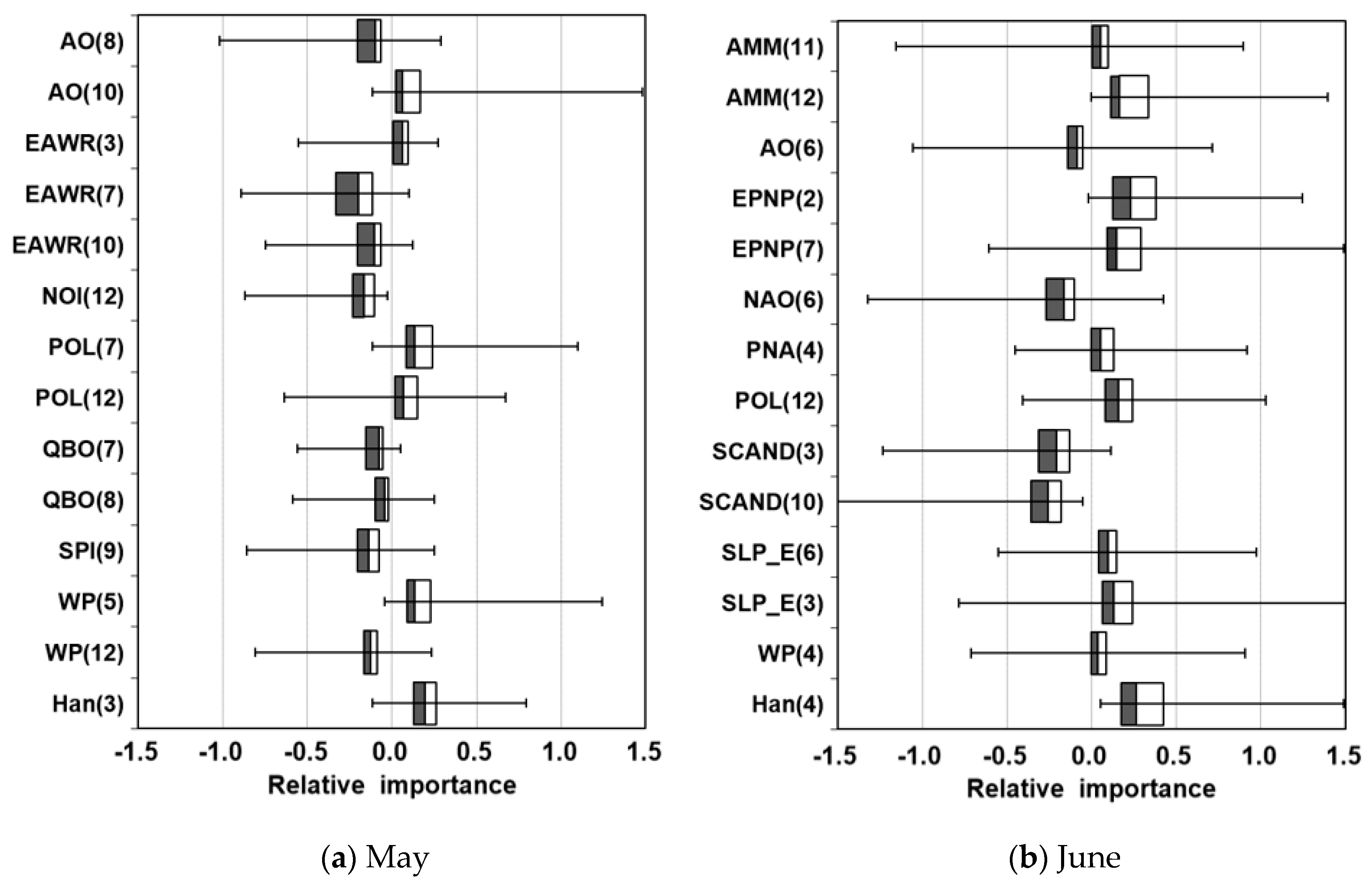
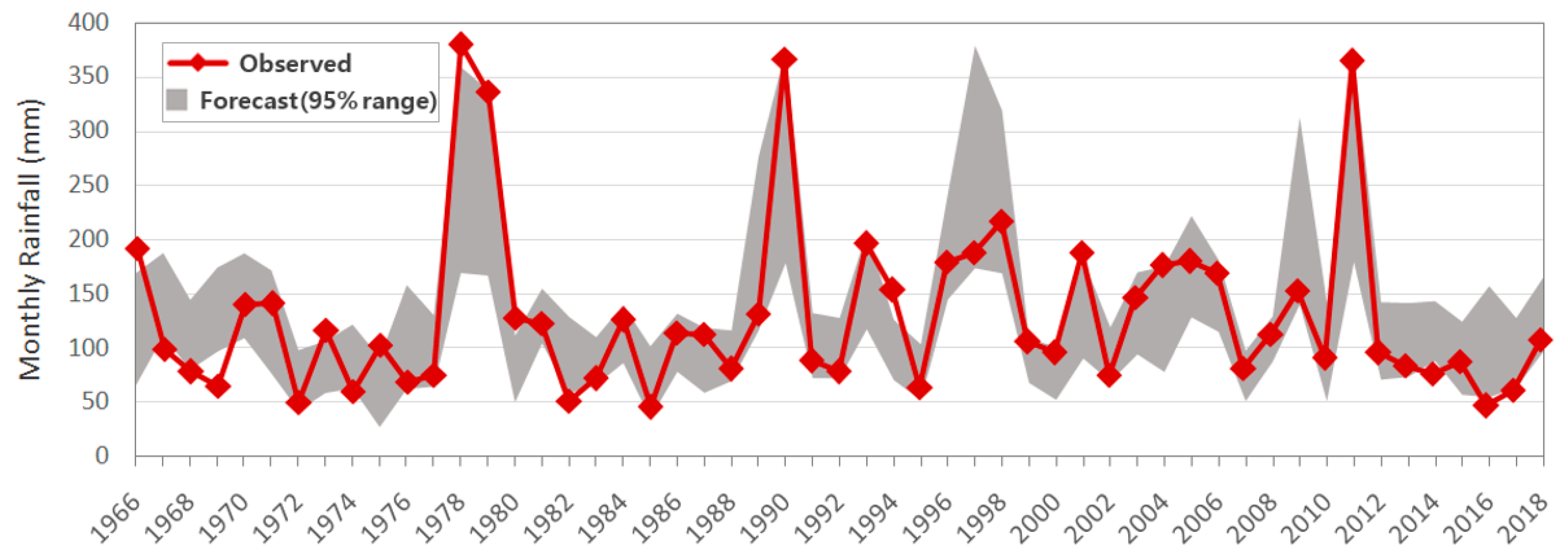
3.3. Uncertainty of the Artificial Neural Network (ANN) Models

To assess the uncertainty of the model outputs, the 95% prediction intervals were estimated using the ensemble of the rainfall forecasts from the ANN-M and ANN-J models. Figure 5 compares the observed rainfall data in May and the forecasted ensembles with the optimal ANN-M model for the entire datasets. The line with a symbol represents the observed data of the monthly rainfall in May, and the shaded area represents the 95% prediction interval. The overall forecast values exhibited the general behavior of the observed values. The estimated prediction interval reasonably represents the observed data, although observations tend to exceed some of the upper and lower limits of the prediction interval in some years and are rather overestimated in years with low rainfall. ANN-M was able to produce ensembles with 58.5% of the total observed data points lying within the prediction interval. The ANN-M produced a reasonable uncertainty band even though the observed values included in the uncertainty band are theoretically less than the expected value of the confidence level. The width of the predictive uncertainty band should be narrower, and the band contains a significant proportion of the observations. The AW of the band is estimated as 50.0 mm, which is acceptable because its standardized value (SAW = 1.03) is closer to the upper criteria of 1.0, which was proposed by Singh et al. [36].

Figure 6 illustrates the 95% uncertainty band of the rainfall forecasts in June using the optimal ANN-J along with the observations. It is clear from the figure that the overall predictions are well-suited to the observed data, and many points of the observed data fall within the prediction interval of the ensembles. It may also be noted that the model is insufficient to produce extremely high and low rainfall characteristics. This may be due to more training sample data in the middle rainfall amount near the normal. The ANN-J model generates ensembles with 67.9% of the observed rainfall data lying within the uncertainty band. The 95% uncertainty band for the June prediction has a larger average band width of 83.0 (SAW = 1.04) compared with the corresponding one for May. However, more observations are included inside the band, which can provide a reasonable estimation of the uncertainty of the rainfall forecasts.

The results of the uncertainty analysis indicated that the middle range of rainfall amount near the normal is well-forecasted by the ANN models irrespective of the variation in the training samples. However, the performance for extremely high or low rainfall may not be satisfactory because limited patterns were used for training the networks. These features have also been found in some previous long-term rainfall forecasting studies [1,13]. It is worth mentioning that accurate forecasts for the lower rainfall below the normal condition is important for water resource management and drought risk mitigation. Accordingly, it could be better to use the lower limit of the uncertainty band estimated in this study for practical purposes. In the future, it will be necessary to improve the performance for long-term forecasting of low and high rainfall with additional considerations by finding other influential input variables, applying other data-driven models, using diverse learning algorithms with different hyper-parameters, and combining the use of physically based models.

4. Conclusions

This study presented ANN models based on the MCCVA technique for forecasting rainfall in May and June for the Han River basin in South Korea. The MCCVA technique was used to generate different parameters of the ANN models while considering variabilities of the random sampling of training datasets and the random assignment of the initial weights of networks. To build the ANN structures, the most influential input variables of the lagged climate indices and the historical rainfall data were selected through the cross-correlation analysis between the input and output variables and the quantification of the relative contribution of each variable to the output variable. This resulted in 11 types of ANN models that have 4 to 14 input variables. The number of the hidden layer was set to one and the neurons varied from 2 to 10. For each combination of the number of input and hidden neurons, 10,000 ANN models were generated using the MCCVA technique with 100 times data splitting of training, validation, and test datasets and 100 sets for the initial weights. The predictive errors were evaluated to find the optimal rainfall forecasting ANN models for May and June.

The optimal ANN model to forecast the monthly rainfall in May with a three month lead-time was determined to have 4 hidden neurons and 11 input variables of the lagged climate indices such as the Atlantic Meridional Mode (AMM), the East Pacific/North Pacific Oscillation (EPNP), the North Atlantic Oscillation (NAO), and the Scandinavia Pattern (SCAND). The prediction errors of the ensemble of forecasts were acceptable with averaged values of the RMSE of 27.4, 33.6, and 39.5 mm, and the correlation coefficients of 0.809, 0.725, and 0.641 for the training, validation, and test datasets, respectively. The uncertainty band obtained from the ensemble of forecasts has covered 58.5% of the observed rainfall data with an average band width of 50.0 mm. Meanwhile, the best ANN rainfall forecasting model, which is two months in advance of June, has 3 hidden neurons and 9 input variables including the Atlantic Meridional Mode (AMM), the East Pacific/North Pacific Oscillation (EPNP), the North Atlantic Oscillation (NAO), and the Scandinavia Pattern (SCAND), which are significantly different from the May model. The averaged RMSE values of the model are 39.5, 46.1, and 62.1 mm, and the correlation coefficients values are 0.853, 0.771, and 0.683 for the training and test datasets, respectively. The results indicate that the uncertainty band for the June rainfall forecasts has coverage of 67.9% with an average band width of 83.0 mm, which are slightly larger than those obtained for May. Both ANN models provide satisfactory forecasting performance despite the limited short learning data that were used. It is discovered that the middle rainfall near normal can be well-bracketed by the estimated prediction interval; however, extremely high or extremely low rainfall is expected to be outside the band. Further research will be required to improve the performance of the ANN models to capture extremely high and low rainfall characteristics. This can be achieved by inputting other climate indices so they can play an important role, have varying time scales, pre-processing the learning data, and combining the use of other statistical models.

It can be concluded that the ANN models with MCCVA enable us to construct a reasonable prediction uncertainty interval as well as to provide an ensemble of rainfall forecasts with improved reliability by reducing variance. The ANN forecasting models developed for the study area are expected to be used for effective and timely water resource management during May and June, which are prone to drought.

References

1. Mekanik, F.; Imteaz, M.A.; Gato-Trinidad, S.; Elmahdi, A. Multiple regression and artificial neural network for long-term rainfall forecasting using large scale climate modes. J. Hydrol. 2013, 503, 11–21. [Google Scholar] [CrossRef]
2. Gholizadeh, M.H.; Darand, M. Forecasting precipitation with artificial neural networks (Case Study: Tehran). J. Appl. Sci. 2009, 9, 1786–1790. [Google Scholar] [CrossRef] [Green Version]
3. Redmond, K.T.; Koch, R.W. Surface climate and streamflow variability in the western United States and their relationship to Large-Scale circulation Indices. Water Resour. Res. 1991, 27, 2381–2399. [Google Scholar] [CrossRef]
4. Schepen, A.; Wang, Q.J.; Robertson, D. Evidence for using lagged climate indices to forecast Australian seasonal rainfall. J. Clim. 2012, 1230–1246. [Google Scholar] [CrossRef]
5. Karabork, M.C.; Kahya, E.; Karaca, M. The influences of the Southern and North Atlantic Oscillations on climatic surface variables in Turkey. Hydrol. Process. 2005, 19, 1185–1211. [Google Scholar] [CrossRef]
6. Abbot, J.; Marohasy, J. Application of artificial neural networks to rainfall forecasting in Queensland, Australia. Adv. Atmos. Sci. 2012, 29, 717–730. [Google Scholar] [CrossRef]
7. Abbot, J.; Marohasy, J. Using lagged and forecast climate indices with artificial intelligence to predict monthly rainfall in the Brisbane Catchment, Queensland, Australia. Int. J. Sustain. Dev. Plan. 2015, 10, 29–41. [Google Scholar] [CrossRef]
8. Abbot, J.; Marohasy, J. Forecasting of monthly rainfall in the Murray Darling Basin, Australia: Miles as a case study. WIT Trans. Ecol. Environ. 2015, 197, 149–159. [Google Scholar]
9. Abbot, J.; Marohasy, J. Application of artificial neural networks to forecasting monthly rainfall one year in advance for locations within the Murray Darling basin, Australia. Int. J. Sustain. Dev. Plan. 2017, 12, 1282–1298. [Google Scholar] [CrossRef] [Green Version]
10. Kumar, D.N.; Reddy, M.J.; Maity, R. Regional rainfall forecasting using large scale climate teleconnections and artificial intelligence techniques. J. Intell. Syst. 2007, 16, 307–322. [Google Scholar]
11. Hartmann, H.; Becker, S.; King, L. Predicting summer rainfall in the Yangtze River basin with neural networks. Int. J. Climatol. 2008, 28, 925–936. [Google Scholar] [CrossRef]
12. Yuan, F.; Berndtsson, R.; Uvo, C.B.; Zhang, L.; Jiang, P. Summer precipitation prediction in the source region of the Yellow River using climate indices. Hydrol. Res. 2016, 47, 847–856. [Google Scholar] [CrossRef] [Green Version]
13. Lee, J.; Kim, C.-G.; Lee, J.E.; Kim, N.W.; Kim, H. Application of Artificial Neural Networks to Rainfall Forecasting in the Geum River Basin, Korea. Water 2018, 10, 1448. [Google Scholar] [CrossRef] [Green Version]
14. Zahmatkesh, Z.; Goharian, E. Comparing machine learning and decision making approaches to forecast long lead monthly rainfall: The city of Vancouver, Canada. Hydrology 2018, 5, 10. [Google Scholar] [CrossRef] [Green Version]
15. Picard, R.R.; Cook, R.D. Cross-validation of regression models. J. Am. Stat. Assoc. 1984, 79, 575–583. [Google Scholar] [CrossRef]
16. Shao, J. Linear model selection by cross-validation. J. Am. Stat. Assoc. 1993, 88, 486–494. [Google Scholar] [CrossRef]
17. Xu, Q.S.; Liang, Y.Z.; Du, Y.P. Monte Carlo cross-validation for selecting a model and estimating the prediction error in multivariate calibration. J. Chemom. 2004, 18, 112–120. [Google Scholar] [CrossRef]
18. Barrow, D.K.; Crone, S.F. Cross-validation aggregation for combining autoregressive neural network forecasts. Int. J. Forecast. 2016, 32, 1120–1137. [Google Scholar] [CrossRef] [Green Version]
19. WAMIS. Available online: https://web.archive.org/web/20200601094620/ (accessed on 31 May 2020).
20. Maier, H.R.; Dandy, G.C. Neural networks for the prediction and forecasting of water resources variables: A review of modelling issues and applications. Environ. Model. Softw. 2000, 15, 101–124. [Google Scholar] [CrossRef]
21. Kim, J.S.; Jain, S.; Yoon, S.K. Warm season streamflow variability in the Korean Han River Basin: Links with atmospheric teleconnections. Int. J. Climatol. 2012, 32, 635–640. [Google Scholar] [CrossRef]
22. Kim, B.S.; Kim, B.K.; Kwon, H.H. Assessment of the impact of climate change on the flow regime of the Han River basin using indicators of hydrologic alteration. Hydrol. Processes 2011, 25, 691–704. [Google Scholar] [CrossRef]
23. Kim, M.K.; Kim, Y.H.; Lee, W.S. Seasonal prediction of Korean regional climate from preceding large-scale climate indices. Int. J. Climatol. 2007, 27, 925–934. [Google Scholar] [CrossRef]
24. CPC. Available online: https://psl.noaa.gov/data/climateindices/list/ (accessed on 31 May 2020).
25. De Veaux, R.D.; Ungar, L.H. Multicollinearity: A Table of Two Nonparametric Regression; Springer: New York, NY, USA, 1994; pp. 393–402. [Google Scholar]
26. Xu, L.; Chen, N.; Zhang, Z.; Chen, Z. A data-driven multi-model ensemble for deterministic and probabilistic precipitation forecasting at seasonal scale. Clim. Dyn. 2020, 54, 3355–3374. [Google Scholar] [CrossRef]
27. Badr, H.S.; Zaitchik, B.F.; Guikema, S.D. Application of statistical models to the prediction of seasonal rainfall anomalies over the Sahel. J. Appl. Meteorol. Climatol. 2013, 53, 614–636. [Google Scholar] [CrossRef] [Green Version]
28. Santos, T.S.; Mendes, D.; Torres, R.R. Artificial neural networks and multiple linear regression model using principal components to estimate rainfall over South America. Nonlinear Processes Geophys. 2016, 23, 13–20. [Google Scholar] [CrossRef]
29. Ahmadi, A.; Han, D.; Lafdani, E.K.; Moridi, A. Input selection for long-lead precipitation prediction using large-scale climate variables: A case study. J. Hydroinform. 2015, 17, 114–129. [Google Scholar] [CrossRef]
30. Lin, F.J. Solving multicollinearity in the process of fitting regression model using the nested estimate procedure. Qual. Quant. 2008, 42, 417–426. [Google Scholar] [CrossRef]
31. Kim, T.W.; Valdes, J.B. Nonlinear model for drought forecasting based on a conjunction of wavelet transforms and neural networks. J. Hydrol. Eng. 2003, 8, 319–328. [Google Scholar] [CrossRef] [Green Version]
32. Olden, J.D.; Joy, M.K.; Death, R.G. An accurate comparison of methods for quantifying variable importance in artificial neural networks using simulated data. Ecol. Model. 2004, 178, 389–397. [Google Scholar] [CrossRef]
33. De Oña, J.; Garrido, C. Extracting the contribution of independent variables in neural network models: A new approach to handle instability. Neural Comput. Appl. 2014, 25, 859–869. [Google Scholar] [CrossRef]
34. National Weather Service. Available online: https://www.weather.gov/mdl/verification_ndfd_public_scoredef#hss (accessed on 31 May 2020).
35. Tokar, A.S.; Johnson, P.A. Rainfall-runoff modeling using artificial neural networks. J. Hydrol. Eng. 1999, 4, 232–239. [Google Scholar] [CrossRef]
36. Singh, A.; Imtiyaz, M.; Isaac, R.K.; Denis, D.M. Assessing the performance and uncertainty analysis of the SWAT and RBNN models for simulation of sediment yield in the Nagawa watershed, India. Hydrol. Sci. J. 2014, 59, 351–364. [Google Scholar] [CrossRef]
37. Tukey, J.W. Exploratory Data Analysis; Addison-Wesley: Boston, MA, USA, 1977. [Google Scholar]
Figure 1. Map of the Han River basin.
Water 12 01743 g001
Figure 2. Relative importance of the input variables obtained using the connection weight method for the rainfall in (a) May and (b) June.
Water 12 01743 g002
Figure 3. Performance of ANN-M model (a) root mean squared error (b) correlation coefficient.
Water 12 01743 g003
Figure 4. Performance of the ANN-J model (a) root mean squared error (b) correlation coefficient.
Water 12 01743 g004
Figure 5. 95% prediction uncertainty interval of the monthly rainfall in May.
Water 12 01743 g005
Figure 6. 95% prediction uncertainty interval of the monthly rainfall in June.
Water 12 01743 g006