Article

Modeling Approaches for Determining Dripline Depth and Irrigation Frequency of Subsurface Drip Irrigated Rice on Different Soil Textures

Department of Chemical and Agricultural Engineering and Technology, University of Girona, Carrer Maria Aurèlia Capmany, 61, 17003 Girona, Catalonia, Spain
*
Author to whom correspondence should be addressed.
Water 2020, 12(6), 1724; https://doi.org/10.3390/w12061724
Submission received: 10 May 2020 / Revised: 13 June 2020 / Accepted: 15 June 2020 / Published: 17 June 2020

Abstract

:
Water saving techniques such as drip irrigation are important for rice (Oriza sativa L.) production in some areas. Subsurface drip irrigation (SDI) is a promising alternative for intensive cropping since surface drip irrigation (DI) requires a higher degree of labor to allow the use of machinery. However, the semi-aquatic nature of rice plants and their shallow root system could pose some limitations. A major design issue when using SDI is to select the dripline depth to create appropriate root wetting patterns as well as to reduce water losses by deep drainage and evaporation. Soil texture can greatly affect soil water dynamics and, consequently, optimal dripline depth and irrigation frequency needs. Since water balance components as deep percolation are difficult to estimate under field conditions, soil water models as HYDRUS-2D can be used for this purpose. In the present study, we performed a field experiment using SDI for rice production with Onice variety. Simulations using HYDRUS-2D software successfully validated soil water distribution and, therefore, were used to predict soil water contents, deep drainage, and plant water extraction for two different dripline depths, three soil textures, and three irrigation frequencies. Results of the simulations show that dripline depth of 0.15 m combined with one or two daily irrigation events maximized water extraction and reduced percolation. Moreover, simulations with HYDRUS-2D could be useful to determine the most appropriate location of soil water probes to efficiently manage the SDI in rice.

1. Introduction

Rice is a main international crops and is a staple food in many countries. Significantly, 90% of worldwide rice production takes place in Asia. In 2018, 67% of the world’s total rice production came from China, India, Indonesia, and Bangladesh [1]. In Europe, Spain is the second largest producer after Italy, with a total surface area of 105,422 ha in 2019 [2].
About 75% of rice is produced under continuous flooded irrigation and uses 34 to 43% of the world’s irrigation water [3]. The total average water use in continuously flooded irrigation can greatly vary depending on the soil type, rice culture, and water management practices, ranging from 6750 m3 ha−1 to 44,500 m3 ha−1 [4].
Water scarcity represents a growing concern in vast producing areas of the world [5]. For this reason, the use of water saving irrigation techniques becomes critical. Alternate wetting and drying irrigation management technique and aerobic rice production systems have shown its effectiveness reducing irrigation needs. Nevertheless, due to the aquatic nature of rice, yield is usually affected. Yields ranging from 1205 to 5664 kg ha−1 have been reported with only 5470–6440 m3 ha−1 of total water input [6]. Great efforts to obtain new rice varieties that combine high yield potential, acceptable grain quality, and drought resistance have been previously carried out [7].
Among irrigation systems, micro-irrigation can supply water accurately, being potentially the most efficient system for growing crops. However, there are few studies dealing with drip irrigation for rice production. He et al. [8] used surface drip irrigation (DI) with NingGeng28 cultivar and obtained a yield of 5785 kg ha−1 applying to 11,215 m3 ha−1 of water, which represents a water productivity that only considers 0.52 kg m−3 of irrigation water (WPIrr). These yields are lesser than those obtained with continuous flooding irrigation (CFI) in the same area (about 8300 kg ha−1), but the WPIrr obtained with DI was doubled. In India, Parthasarathi et al. [9] found an average yield of 4834 kg ha−1 with a water productivity considering the irrigation and rain WPIrr+R = 0.84 kg m−3 using DI with ADT(R) 45 variety. In Spain, using DI with the Baldo variety, Arbat et al. [10] obtained 5565 kg ha−1 and a WPIrr+R of 0.60 kg m−3. Nevertheless, DI hindered the passage of machinery due to the driplines laying on the soil surface, forcing a withdrawal of the driplines before sowing the following season. Subsurface drip irrigation (SDI) may overcome these inconveniences because driplines are protected below the soil surface and can last several years [11]. However, if driplines are installed too deep, germination and development of shallow-rooted crops can be difficult [12]. Rajwade et al. [13] and Parthasarathi et al. [9] both studied SDI for rice production. In the former, driplines were spaced 0.4 and 0.6 m apart, and emitters were space 0.3 m apart. Emitter discharge was 4 L h−1 but dripline depth was not specified [13]. In the latter study, driplines were spaced 0.6, 0.8, and 1.0 m apart, while emitter discharges were 0.6 and 1.0 L h−1. Emitter spacing was 0.3 m and dripline depth was 0.15 m [9]. Both studies concluded that SDI yield was slightly reduced compared with conventional CFI, even though water productivity was increased.
In crops with deep rooting systems, like sunflower, soybean, and grain sorghum, previous studies did not show differences in yield and WP between 0.2 and 0.6 m dripline depths when crop germination and establishment were not limited [12]. The main reasons for shallower dripline placement is to allow for better crop germination and establishment as well as to cultivate shallow rooted crops such as horticultural crops [14]. While rice does not have deep roots, the use of SDI can promote deeper rooting development as a strategy to increase drought resistance [15].
There is practically no information about the most appropriate depth and spacing at which driplines, emitter spacing and discharge, and duration of the irrigation events with rice should be installed. Therefore, it is necessary to establish design and irrigation management criteria to maximize grain yield and minimize water losses.
Numerical models that solve the Richards equation have been used to analyze soil water distribution under different irrigation systems and strategies for many years [16], as well as to estimate major components of field water balance [17]. They have the advantage of reducing cost and time of the field experiments [18]. Different models, such as DAISY [19], COUP [20], SWAP [21], SALTMED [22], and HYDRUS [23], have been developed and are being used for this purpose. HYDRUS software packages [23] have been widely and successfully used to simulate soil water distribution under different irrigation systems, soil types, and management strategies [24]. HYDRUS defines complicated flow domains in one, two, or three dimensions (1D, 2D, and 3D), and allows for flexible boundary conditions using a friendly graphical user interface. This model has been used to simulate different irrigation types, such as continuous flooding irrigation [17], furrow irrigation [25,26,27], sprinkler irrigation [28,29,30], surface drip irrigation [31,32,33], and subsurface drip irrigation [34,35,36].
Under continuous flooding irrigation (CFI), which is commonly used in paddy rice, soil water movement can be assumed as one-dimensional (1D). Thus, HYDRUS-1D, has been shown to adequately predict soil water potential, evapotranspiration, and deep percolation in continuous flooding rice irrigation [17,18,19]. Nevertheless, the water movement under SDI needs a two-dimensional (2D) or three-dimensional (3D) approach. Generally, when emitters are close to each other along the dripline an infinite line source is considered and a 2D model is applied [37,38,39].
Reyes-Esteves and Slack [34] used HYDRUS-2D to simulate spatial and temporal distributions of soil water contents, root water uptake of an SDI system commonly used for alfalfa production in California. In this work, the depth at which driplines must be placed in alfalfa was optimized considering different scenarios of irrigation patterns and soil textures. At the knowledge of the authors there are no previous applications of HYDRUS-2D on rice production using subsurface drip irrigation.
The general objectives of this work were to determine the depth at which driplines should be installed, to establish the most effective irrigation frequency for rice production using SDI in soils of different textures, and to estimate major components of the field water balance. Field experiments and simulations with HYDRUS-2D were carried out for these purposes.

2. Materials and Methods

2.1. Field Experiment

Field tests were carried out in Pals (Baix Ter, Girona, Spain) during 2019 growing season on an experimental plot of 0.39 ha (41°58′43″ N, 3°08′21″ E). The soil texture of the plot was spatially heterogeneous; sandy-loam textural class prevailed in 85% of the surface area of the experimental field and loamy one in the other 15% (Table 1). In addition, another soil of silty-clay texture was characterized (Table 1) since it was also representative of the Baix Ter production area, with the further objective of extrapolating the results obtained in the field test with the HYDRUS-2D simulation results.
The SDI system was installed with driplines buried at 0.15 m and spaced 0.66 m. Thin-walled driplines (0.38 mm), 16.20 mm internal diameter with integrated pressure-compensating emitters of 1 L h−1 (Dripnet PCTM AS, Netafim, Israel), spaced 0.3 m apart, were used.
The plot was sowed on 28 May 2019 using the variety Onice on dry soil conditions with a seed drill at 135 kg ha−1 and spacing the seeding lines 0.19 m. The general irrigation criteria was based on maintaining −10 kPa of soil water potential at 0.10 m depth and at a horizontal distance of 0.08 m from the emitter (Figure 1). This matric potential corresponds to the field capacity for aerobic rice [40].
Temperature, rainfall, atmospheric pressure, air humidity, global radiation, and wind speed were measured with an automated meteorological station, located approximately 2 km from the experimental plot. The reference evapotranspiration (ETo) was determined using the FAO-56 method [41], which requires solar radiation, maximum, minimum, and mean air temperatures, air humidity, and wind speed data measured with the automated meteorological station.
Irrigation water applied to the plot was continuously measured using a volumetric meter. Soil water contents were continuously determined from day 34 after sowing (DAS), at 0.10 and 0.25 m depths and in two horizontal positions, one close to the emitter, at 0.08 m from the dripline, and the other at the intermediate region between the two driplines (Figure 1). Volumetric soil water contents were measured using a sensor based on frequency domain reflectometry, with an accuracy of ±3% (SM 150-T, Delta-T Devices, Cambridge, UK). Sensors were located in part of the plot with a sandy-loam texture. Depth of the water table was monitored with weekly readings in 3 piezometers, 2 m long, located around the plot, which allowed to establish adequate boundary conditions in simulations, as explained in Section 2.2.
Phenological stages of the crop were monitored throughout the campaign. Yield was obtained from sampling carried out on 18 October 2019, at the stage of physiological maturity. Six samples were taken on a reference surface of 0.5 m × 0.5 m for each of the two soil textures present in the plot (sandy-loam and loam, Table 1). After drying the samples, standardized production was obtained at a grain humidity of 14%. Average productions in the surfaces corresponding to each textural class were determined, carrying out an analysis of variance to find out the existence of significant differences depending on soil texture.
Water productivity (WP), which characterizes yield (Y) per unit of water used, was calculated in two ways:
W P I r r + R = Y I r r + R
W P I r r = Y I r r
being Y the rice grain yield at 14% of humidity (kg ha−1); Irr the irrigation water (m3 ha−1); and R the precipitation during the cultivation period (m3 ha−1).

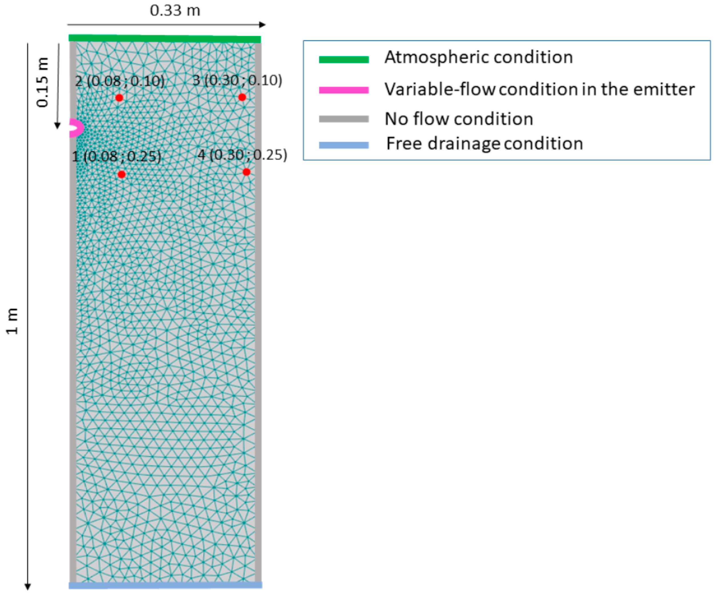
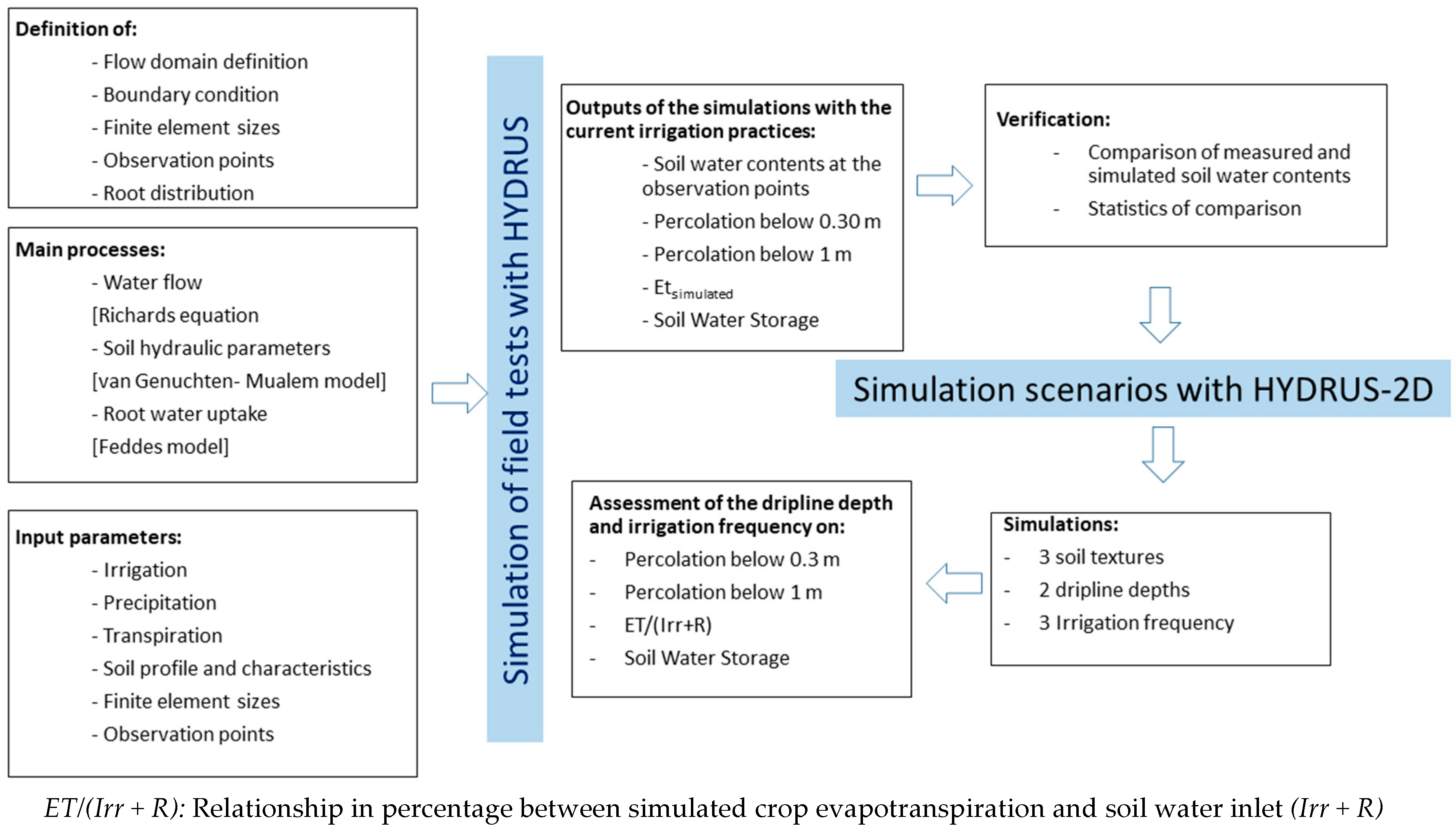
2.2. Simulations of Soil Water Dynamics

In order to model soil water dynamics, HYDRUS-2D [42] was selected. Due to the short distance between two consecutive emitters along the dripline (0.3 m), soil water movement can be assumed as two-dimensional. This well-known software package solves numerically Richards equation:
θ t = x [ K ( h ) h x ] + z [ K ( h ) h z + K ( h ) ] S ( h )
where θ is the volumetric soil water content (m3 m−3), t is the time (day), x and z the spatial horizontal and vertical coordinates (m), respectively, h the soil water pressure (m), K(h) the hydraulic conductivity function (m day−1), and S(h) the sink term in the equation (m3 m−3 day−1), to consider plant water extraction.
Soil water retention and hydraulic conductivity functions were determined following the van Genuchten–Mualem model [43]. The parameters of the equations are shown in Table 2 and were estimated with Rosetta [44] from the percentages of sand, silt, and clay. Bulk density and water content were at −33 and −1500 kPa (Table 1).
A flow domain 1 m deep and 0.33 m wide was considered, going from the vertical line where the dripline was located to the intermediate position between two driplines. Spatial discretization was performed with triangular elements with a dimension close to 0.001 m in the area closest to the emitter up to approximately 0.020 m in the area furthest away. In all simulations, initial condition in the whole domain was fixed as a matric potential of −33 kPa, corresponding to the initial conditions in the field test in the sandy-loam textured soil. In order to compare the results with the ones of the rest of simulated scenarios, the same initial condition was used. The boundary conditions were absence of flow on the two sides of the domain, unit vertical hydraulic gradient simulating free drainage from the bottom of the domain since, according to the piezometer readings, the depth of the aquifer was always greater than 2 m, and an atmospheric boundary condition at the soil surface. In the elements representing the emitter, a variable flow condition was considered over time, in which the flow-rate during irrigation periods was obtained according to:
F = q d   ·   2 · π   ·   r   = 0.024   m 3   day 1 0.30   m     ·   2   m   ·   π   ·   0.0085   m = 1.498   m   day 1
being F, the water-flow applied to the variable condition in the emitter zone (m day−1); q emitter discharge (m3 day−1); d emitter spacing (m); and r external radius of the dripline (m).
In addition to the simulated field tests, different scenarios collected in the A–V cases listed in Table 4 were considered: two dripline depths (0.15 and 0.25 m) and three different soil textures (silty-clay, loam, and sandy-loam) that were representative of Baix Ter rice production area. It should be noted that the depths considered for the driplines are compatible with the cultural tasks foreseen.
Simulated irrigation practices were: (1) irrigation practiced during 2019 campaign (cases A–C, Table 4); (2) irrigation based strictly on crop evapotranspiration applying three different irrigation frequencies: two irrigations per day, one daily irrigation, and one irrigation every four days (Cases D–V, Table 4). A conceptual figure showing input and output parameters and followed procedure for the set of simulations carried out is depicted in Figure 2.
Climatic data from sowing (18 May 2019) to harvest (18 October 2019) was considered. Crop evapotranspiration (ETc) was determined to consider water extraction in simulations according to the equation:
E T c = E T o · K c
being Kc the crop coefficient, determined for the reference region following the suggested values by Allen et al. [41].
HYDRUS-2D code requires evaporation and transpiration as two independent input terms, since evaporation is treated as a surface boundary condition and transpiration as the sink term in the Richards equation. For a crop that does not cover the entire surface, which happened from sowing time up to 70 days later, the potential evapotranspiration is divided between potential evaporation (Ep) and potential transpiration (Tp). The partition of these two terms was carried out using the leaf area index (LAI), following the procedure described in the SWATRE model and using the equations [45]:
E p = E T c · e K g r · L A I
T p = E T c E p
Global solar radiation coefficient in rice (Kgr) was set to 0.3 according to Li et al. [17] and Phogat et al. [46]. LAI values were determined based on the phenological stages observed in the same plot and with the same variety of rice during the 2018 irrigation season. LAI values were obtained every two weeks using PocketLAI [47]. During the simulated periods in which there was no crop and potential evaporation was considered to be equal to ETo.
Water extracted by the crop was determined according to the equations proposed by Feddes [48] and with the optimized response parameters for rice crop obtained by Singh et al. [49] and applied, among others, by Li et al. [50]. It was considered that water extraction was located at the depth where the rice root system develops, being more intense near the soil surface and decreasing towards the maximum rooting depth, which was 0.25 m, according to field observations throughout the irrigation season.

2.3. Validation of the Simulation Model

HYDRUS-2D model was validated by comparing simulated soil water contents with soil water contents measured in the experimental plot at the positions described in Section 2.1. The validation period included the whole irrigation campaign and after the harvest, from 1 July 2019, when sensors were installed, until 22 January 2020. The root of the mean square error (RMSE), normalized RMSE (nRMSE), the coefficient of determination (R2) and Nash–Sutcliffe model efficiency coefficient (E) were calculated to quantify the goodness of model predictions as follows:
R M S E = i = 1 n ( P i O i ) 2 n
n R M S E = R M S E O ¯ · 100
R 2 = { i = 1 n ( O i O ¯ ) ( P i P ¯ ) [ i = 1 n ( O i O ¯ ) 2 ] 0.5   [ i = 1 n ( P i P ¯ ) 2 ] 0.5   } 2
E = 1 i = 1 n ( O i P i ) 2 i = 1 n ( O i O ¯ ) 2
where Pi are simulated values, Oi are observed values, O ¯ is the mean of observed values, P ¯ is the mean of predicted values, and n is the total number of observations.
The RMSE indicates the difference between observed and simulated soil water contents. It has the advantage of having the same units as measured value and therefore it can be compared with it. A lower value of RMSE indicates a good prediction of the model, meaning a value of zero is a perfect fit. The nRMSE relativizes the root mean square error value, dividing it by the mean of the observed values. When nRMSE is less than 10%, the prediction of the model is excellent, whereas the prediction is good if its value ranges between 10–20%. Further, the prediction is fair if it is greater than 20% and lower than 30%, and poor when it is greater than 30% [51,52]. E means it has been extensively used to evaluate the performance of hydraulic models, ranging its values from −∞ to 1, with greater values indicating better agreement. When E equals zero the observed mean O ¯ is as good as a predictor as the model. When E is negative it indicates that O ¯ is a better predictor than the model [53,54].

2.4. Water Balance Components

Simulation of soil water dynamics in the experimental plot and in the considered scenarios allowed the assessment of the water balance throughout the cultivation period (from the day of planting to harvesting, 144 days in total) considering water inlets (rain (R) and irrigation (Irr)) as well as outlets (drainage below 1 m and crop evapotranspiration). In addition, variation of soil water storage in the entire soil profile, error in the water balance of the model and the water that drained below 0.3 m depth (which was considered not usable by the crop, due to the depth of the rice rooting system) were computed. The relationship between cumulative evapotranspiration computed by the model (ETsim) and water inlets in the soil profile was also determined. (ETsim/(Irr + R))·100 shows the percentage of water evapotranspirated in relation to contributions of water from irrigation and rain (Irr + R), being desirable to maximize its value to increase water use efficiency.

3. Results and Discussion

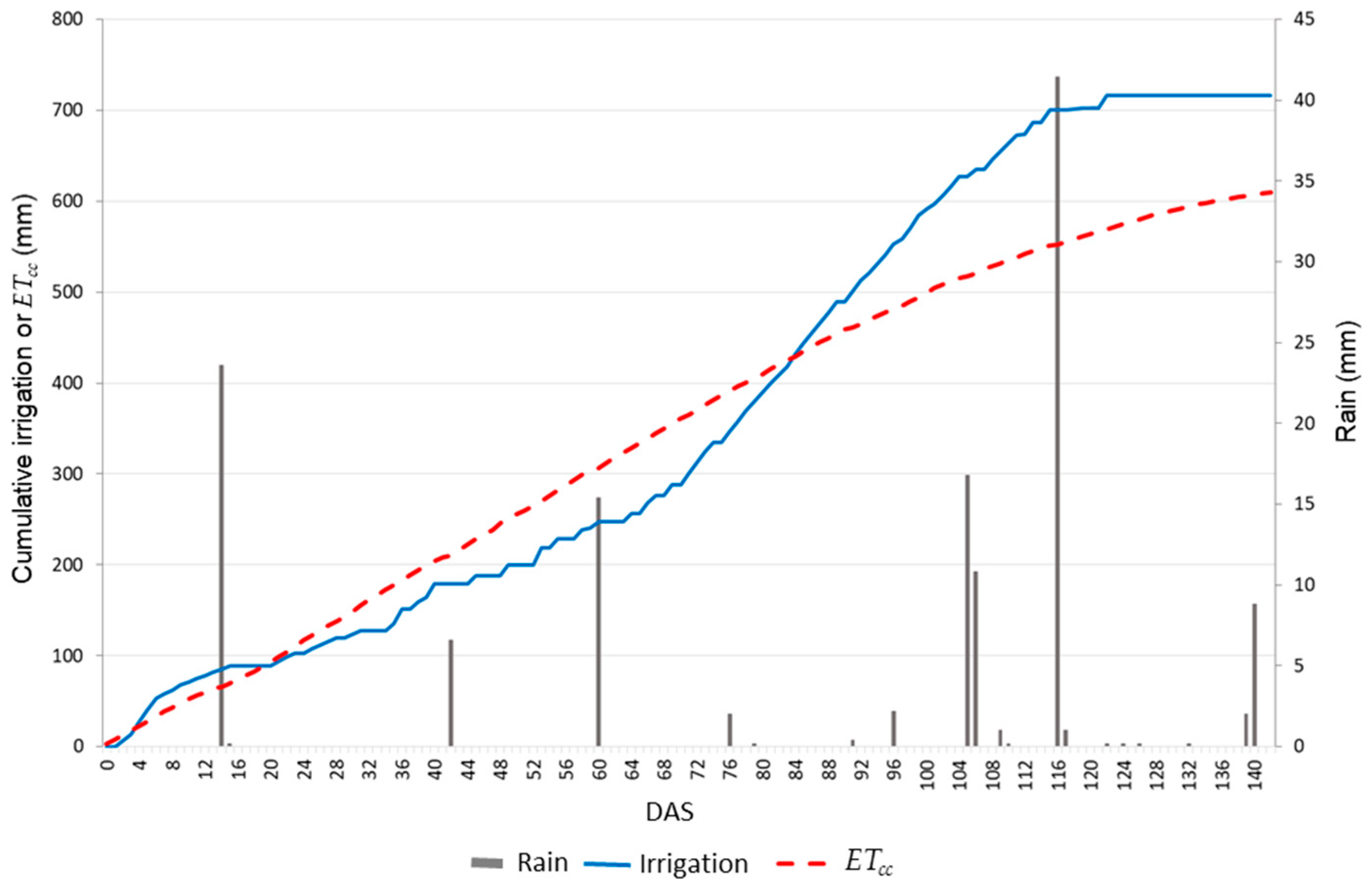
3.1. Irrigation Campaign in the Experimental Plot

Suitability of the irrigation pattern followed during the growing season is analyzed in this section. The amount of water supplied by irrigation during the first three weeks was higher than evapotranspiration demand (Figure 2). The reason for this was the need to promote seed germination after sowing. From day 15 to 70 DAS (from 12 June to 6 August 2019), the plot was watered in order to maintain the soil water content in sensor 2 (Figure 1) at 0.257 m3 m−3, corresponding to a matric potential of −10 kPa, resulting in cumulative applied irrigation water was lower than cumulative crop water demand (ETcc) (Figure 3). To correct this problem, the irrigation schedule was modified from day 70 to 123 and during this period a slightly higher irrigation water amount than that of the extractions estimated from the ETc was provided. Consequently, from day 84 the accumulated irrigation surpassed the cumulative ETc again (Figure 3). From day 123 until day 140, irrigation was stopped as the crop reached physiological maturity and the goal was to reduce the grain humidity in order to harvest as soon as possible.
Soil water contents measured at different positions from the dripline (Figure 1) are shown in Figure 4. The matric potential at 0.08 m from the dripline and at 0.10 m depth was found above −10 kPa (corresponding to a volumetric content of 0.257 m3 m−3) during the entire growing period (from 34 to 140 days DAS). Therefore, it should not suppose a reduction of potential yield according to Bouman et al. (2005) [40], as this water potential corresponds to field capacity for aerobic rice. At the same distance from the dripline but at a depth of 0.25 m, the matric potential was below −20 kPa (corresponding to 0.21 m3 m−3) practically throughout the entire crop cycle. With this value of matric potential, notable reductions in production were expected according to Cabangon et al. (2003) [55].
In the furthest measurement points from the dripline (positions 3 and 4), the matric potential was also below −20 kPa between 34 and 70 DAS, corresponding to the period where irrigation water supply was lesser than ETc, meaning that the crop might be seriously stressed in the area located between driplines.

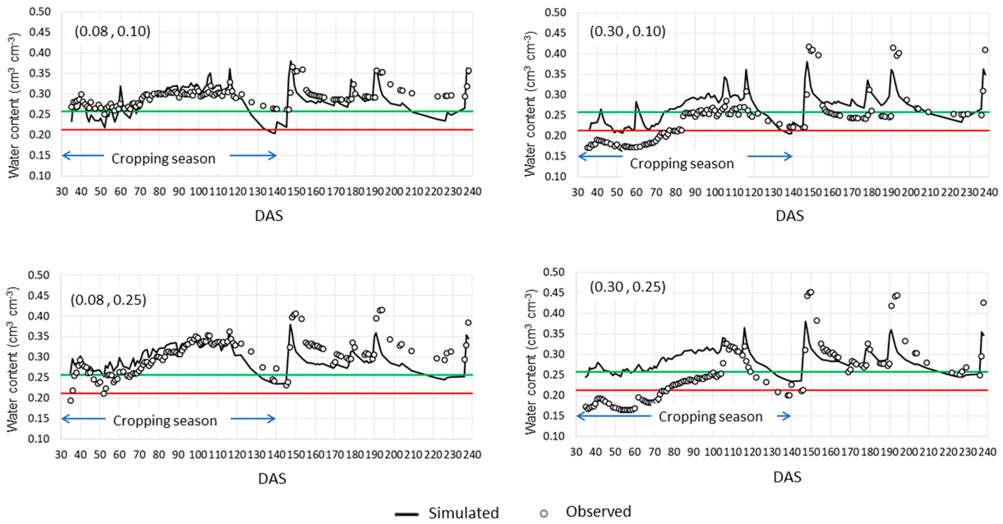
3.2. Validation of the Model

The visual comparison of the simulated and observed soil water contents in the experimental plot showed a similar trend (Figure 4), which illustrates a good performance of the model. Root mean square error (RMSE) values ranging from 0.028 m3 m−3 and 0.064 m3 m−3, nRMSE ranged from 9.4% to 25.3%, determination coefficients (R2) ranging from 0.38 and 0.54 and E from −0.589 to 0.353 (Table 3). Only in the positon (0.08, 0.10) the value of E was negative, meaning that the observed mean is a better predictor than the model. Nevertheless, the nRMSE in this case was less than 10% which indicates and excellent performance of the model. The greatest differences were found from 30 to 100 days after sowing in the area furthest from the dripline, where the observed soil water contents were systematically higher than that simulated with HYDRUS-2D.
The statistics of comparison are similar to those obtained in previous works in which the observed and simulated soil water contents were compared in bare soil [37], in an apple orchard [16], and in laboratory scale experiments [56]. The differences between simulated and measured soil water contents can be explained by different causes, being some of them: (1) the soil variability, (2) the different representative volume of soil explored by the soil water sensor (which has a rod length of 51 mm) and the nodal points where HYDRUS-2D provided the water content, and (3) the accuracy of the measurement techniques.
A calibration of the model with an independent dataset of measurements in the same soil can be used to reduce the differences between measured and simulated soil water contents [18,57]. Nevertheless, calibration requires an independent dataset of soil water measurements obtained in similar conditions which is not always feasible.

3.3. Components of Water Balance and Percolation Below 0.3 m Depth

Table 4 shows the variables that determine water balance terms, simulated cumulative evapotranspiration with HYDRUS-2D (ETsim), percolation below 0.3 m, error and some derived relationships for each one of the analyzed cases, as described in Section 2.4.
Errors in mass balance (BE) calculated as (Inputs + Outputs + SS) in simulations performed with HYDRUS-2D were minimal, the highest one being 12 mm or less than 1.7% (percentage defined as [ B E I r r + R · 100 ] ). These values are slightly lower than those published by Li et al. [17], where the HYDRUS-1D model was used in rice irrigated by flooding. In general, water balance errors were higher in simulations with silty-clay textured soil.
Cumulative ETc computed following Allen et al. [20] (ETcc) throughout 240 days of crop cycle accounted 642 mm (Figure 3), while the cumulative ETc simulated with HYDRUS-2D (ETsim) was among 66 and 86% of the previous one. ETsim was higher in silty-clay and loam soil textures than in sandy-loam and, in general, declined when frequency of between consecutive irrigations decreased and when emitter depth increased, especially in the sandy-loam soil texture. The higher ETsim in loam soil compared with sandy-loam soil texture (cases A and B, Table 4) could be explained by higher grain yield obtained in the part of the field where soil had loam texture. On the other hand, the drained water below 0.3 m depth was higher in the sandy-loam soil than in the loam and silty-clay soil textures, which explains why simulated evapotranspiration and ETsim/(Irr+R) ratios were higher.
In cases where irrigation restored crop evapotranspiration (cases D–V, Table 4) and dripline depth was 0.15 m (D, E, F, J, K, L, P, Q, and R), an increase of the ratio between evapotranspirated water and supplied water ETsim/(Irr+R) was determined in comparison with irrigation patterns observed in the experimental tests (cases A, B, and C), whatever the texture or frequency of irrigation was. This would indicate that following the irrigation criteria to restitute the crop evapotranspiration would have improved the water use by the crop.
Frequency of irrigation had practically no influence on the ETsim in silty-clay soil texture (cases P–V). On the other hand, a slight increase in ETsim/(Irr + R) ratio was observed when increasing the frequency of irrigation in the sandy-loam and loam soil textures. Similarly, an increase in the irrigation frequency reduced drainage below 0.3 m depth. The lower water holding capacity of coarse textured soil may explain the obtained results.
When comparing the 2 dripline depths in a sandy-loam textured soil using the same irrigation frequency, it was observed that 0.15 m depth reduced drainage below 0.30 m, increased the ETsim/(Irr + R) ratio and, consequently, the water used by the plant. This also happened in soils with loamy and silty-clay textures, although to a lesser extent.

3.4. Yield and Water Productivity

Yield in the field showed two differentiated zones corresponding to the diverse soil texture within the same field. In the sandy-loam textured area, yield (734 kg ha−1) was significantly lower (p < 0.05) than the one corresponding to the loam-textured area (5363 kg ha−1). As mentioned in Section 3.1, soil water contents were measured in the sandy-loam part of the field. In the mid-way between two driplines the soil water content achieved values corresponding to matric potential bellow −20 kPa during the period from 34 to 70 DAS (corresponding to from tillering to beginning of flowering stages). Rice is especially sensitive to lack of water during this period, explaining the low yield obtained in the parts of the plot of sandy-loam texture. Furthermore, low water availability in the mid-way between two consecutive driplines in sandy-loam-soil (position 3 in Figure 1), could give a competitive advantage to weeds that have the capacity to develop despite having low amounts of water available. However, the yield of 5363 kg ha−1 and the water productivity (WPIrr+R) of 0.62 kg m−3 in the loam textured part of the field was similar to that obtained in previous irrigation campaign in a field test irrigated by surface drip in a silty-clay textured soil with a very shallow aquifer (Table 5), in which a yield of 5565 kg ha−1 and a WPIrr+R of 0.60 kg m−3 were obtained [10].
Table 5 shows the water productivity in the current field tests with SDI and the results obtained in continuous flooding irrigation (CFI) and surface drip irrigation during the 2017 campaign in the same area.
Under continuous flooding irrigation (CFI) and dry seeding conditions in nearby fields, the same authors reported a yield of 6486 kg ha−1 and a WPIrr+R of 0.42 kg m−3. Although in CFI the yield was 16% higher than in SDI, the WP was similar to that of surface drip irrigation (DI), showing an increase above 40% of the WPIrr+R compared with CFI. Therefore, SDI systems may be of interest in situations where water is a limiting factor.
Among the few published works of rice irrigated using SDI, Rajwade et al. [13] in a sandy-loam soil obtained yields ranging from 1881 to 5074 kg ha−1 and WPIrr+R from 0.23 to 0.61 kg m−3. Parthasarathi et al. [9] in a clay-loamy soil obtained yields of 5600 kg ha−1 with WPIrr+R of 0.86 kg m−3. Although the maximum yields reported by these authors were very similar to each other and to the one obtained in the present work, there is a great difference among the WP values, which could be attributed to different soil textures. In general, coarser soils require higher irrigation water amounts in order to allow water to reach the root system from the emitter.

4. Conclusions

To maximize potential water savings of subsurface drip irrigation (SDI) systems, it is necessary to optimize its design and irrigation management, highlighting depth of emitters and frequency of irrigation. The RMSE and R2 values obtained by comparing the water contents measured in the field and simulated with HYDRUS-2D showed a reasonably good prediction with the latter, indicating that numerical simulations can be: (1) a useful tool to optimize the design and management of SDI taking into account the hydraulic properties of soils, as well as, (2) predicting water percolation. The results of the simulations applied to the production of rice in Baix Ter area considering soils with different texture allowed to determine that the most adequate dripline depth to minimize water losses due to percolation and maximize water extraction by plants is 0.15 m with a high frequency of irrigation, such as one or two irrigation events per day.
On the other hand, location of measurement points is critical when using irrigation criteria based on a matric potential threshold. Indeed, irrigation management based on maintaining a certain potential or water content in a very close location to the emitter can lead to insufficient irrigation. For this purpose, simulations with HYDRUS-2D can be useful to determine the most appropriate location of the soil water probes in order to efficiently manage the SDI in rice.

Author Contributions

Conceptualization, G.A. and F.R.d.C.; methodology, G.A., M.D.-R., and F.R.d.C.; investigation, G.A., M.D.-R., S.C., J.P. (Jaume Pinsach) and J.P. (Joan Pujol); data curation, G.A. and S.C.; writing—original draft preparation, G.A., F.R.d.C., and J.P.-B.; writing—review and editing, all the authors; project administration, J.P. (Jaume Pinsach) and F.R.d.C. All authors have read and agreed to the published version of the manuscript.

Funding

This research was funded by the European Program for Research and Innovation Horizon 2020-PRIMA, grant number PCI2019-103738 (Towards a sustainable use of water in Mediterranean rice-based agro-ecosystems (MEDWATERICE).

Acknowledgments

The authors wish to thank the company Netafim for the technical support received during the field tests.

Conflicts of Interest

The authors declare no conflict of interest.

References

  1. Food and Agriculture Organization of the United Nations. FAOSTAT–Food and Agriculture Data. Available online: http://www.fao.org/faostat/en/#data (accessed on 5 May 2020).
  2. MAPA. Estadísticas de Superficies y Producciones Anuales de Cultivo en España; MAPA: Madrid, Spain, 2018. [Google Scholar]
  3. Maraseni, T.N.; Deo, R.C.; Qu, J.; Gentle, P.; Neupane, P.R. An international comparison of rice consumption behaviours and greenhouse gas emissions from rice production. J. Clean. Prod. 2018, 172, 2288–2300. [Google Scholar] [CrossRef]
  4. Maclean, J.L.; Dawe, D.C.; Hardy, B.; Hettel, G.P. Rice Almanac: Source Book for the Most Important Economic Activity on Earth, 4th ed.; International Rice Research Institute: Los Baños, Philippines, 2013. [Google Scholar]
  5. Zheng, J.; Wang, W.; Ding, Y.; Liu, G.; Xing, W.; Cao, X.; Chen, D. Assessment of climate change impact on the water footprint in rice production: Historical simulation and future projections at two representative rice cropping sites of China. Sci. Total Environ. 2020, 709, 136190. [Google Scholar] [CrossRef]
  6. Bouman, B.A.M.; Yang, X.; Wang, H.; Wang, Z.; Zhao, J.; Chen, B. Performance of aerobic rice varieties under irrigated conditions in North China. Field Crops Res. 2006, 97, 53–65. [Google Scholar] [CrossRef]
  7. Luo, L.; Mei, H.; Yu, X.; Xia, H.; Chen, L.; Liu, H.; Zhang, A.; Xu, K.; Wei, H.; Liu, G.; et al. Water-saving and drought-resistance rice: From the concept to practice and theory. Mol. Breed. 2019, 39. [Google Scholar] [CrossRef]
  8. He, H.; Ma, F.; Yang, R.; Chen, L.; Jia, B.; Cui, J.; Fan, H.; Wang, X.; Li, L. Rice performance and water use efficiency under plastic mulching with drip irrigation. PLoS ONE 2013, 8, e83103. [Google Scholar] [CrossRef] [Green Version]
  9. Parthasarathi, T.; Vanitha, K.; Mohandass, S.; Senthilvel, S.; Vered, E. Effects of impulse drip irrigation systems on physiology of aerobic rice. Indian J. Plant Physiol. 2015, 20, 50–56. [Google Scholar] [CrossRef]
  10. Arbat, G.; Parals, S.; Duran-Ros, M.; Pujol, J.; Puig-Bargués, J.; Ramírez de Cartagena, F. Dinámica del Agua en el Suelo, Productividad del Agua y Economía en Riego por Inundación y Goteo en Arroz; XXXVI Congreso Nacional de Riegos, AERYD: Valladolid, Spain, 2018; Volume 19, pp. 1–10. [Google Scholar]
  11. Lamm, F.R.; Rogers, D.H. Longevity and performance of a subsurface drip irrigation system. Trans. ASABE 2017, 60, 931–939. [Google Scholar] [CrossRef]
  12. Lamm, F.R.; Abou Kheira, A.A.; Trooien, T.P. Sunflower, Soybean, and Grain Sorghum Crop Production as Affected by Dripline Depth. Appl. Eng. Agric. 2010, 26, 873–882. [Google Scholar] [CrossRef]
  13. Rajwade, Y.A.; Swain, D.K.; Tiwari, K.N.; Bhadoria, P.B.S. Grain yield, water productivity, and soil nitrogen dynamics in drip irrigated rice under varying nitrogen rates. Agron. J. 2018, 110, 868–878. [Google Scholar] [CrossRef]
  14. Lamm, F.R.; Trooien, T.P. Dripline Depth Effects on Corn Production When Crop Establishment Is Nonlimiting. Appl. Eng. Agric. 2005, 21, 835–840. [Google Scholar] [CrossRef] [Green Version]
  15. Miyazaki, A.; Arita, N. Deep rooting development and growth in upland rice NERICA induced by subsurface irrigation. Plant Prod. Sci. 2020, 1–9. [Google Scholar] [CrossRef]
  16. Arbat, G.; Puig-Bargués, J.; Barragán, J.; Bonany, J.; Ramírez de Cartagena, F. Monitoring soil water status for micro-irrigation management versus modelling approach. Biosyst. Eng. 2008, 100, 286–296. [Google Scholar] [CrossRef]
  17. Mo’allim, A.A.; Kamal, M.R.; Muhammed, H.H.; Yahaya, N.K.E.; Man, H.B.; Wayayok, A. An assessment of the vertical movement of water in a flooded paddy rice field experiment using Hydrus-1D. Water 2018, 10, 783. [Google Scholar] [CrossRef] [Green Version]
  18. Rezayati, S.; Khaledian, M.; Razavipour, T.; Rezaei, M. Water flow and nitrate transfer simulations in rice cultivation under different irrigation and nitrogen fertilizer application managements by HYDRUS-2D model. Irrig. Sci. 2020. [Google Scholar] [CrossRef]
  19. Abrahamsen, P.; Hansen, S. Daisy: An open soil-crop-atmosphere system model. Environ. Model. Softw. 2000, 15, 313–330. [Google Scholar] [CrossRef]
  20. Jansson, P.E.; Moon, D.S. A coupled model of water, heat and mass transfer using object orientation to improve flexibility and functionality. Environ. Model. Softw. 2001, 16, 37–46. [Google Scholar] [CrossRef]
  21. van Dam, J.C.; Groenendijk, P.; Hendriks, R.F.A.; Kroes, J.G. Advances of Modeling Water Flow in Variably Saturated Soils with SWAP. Vadose Zone J. 2008, 7, 640. [Google Scholar] [CrossRef]
  22. Ragab, R. Integrated Management Tool for Water, Crop, Soil and N-Fertilizers: The Saltmed Model. Irrig. Drain. 2015, 64, 1–12. [Google Scholar] [CrossRef] [Green Version]
  23. Šimůnek, J.; van Genuchten, M.T.; Šejna, M. Recent Developments and Applications of the HYDRUS Computer Software Packages. Vadose Zone J. 2016, 15, 2–25. [Google Scholar] [CrossRef] [Green Version]
  24. Karandish, F.; Šimůnek, J. A field-modeling study for assessing temporal variations of soil-water-crop interactions under water-saving irrigation strategies. Agric. Water Manag. 2016, 178, 291–303. [Google Scholar] [CrossRef] [Green Version]
  25. Bristow, K.L.; Šimůnek, J.; Helalia, S.A.; Siyal, A.A. Numerical simulations of the effects furrow surface conditions and fertilizer locations have on plant nitrogen and water use in furrow irrigated systems. Agric. Water Manag. 2020, 232, 124. [Google Scholar] [CrossRef]
  26. Sanchez, C.A. Modeling Flow and Solute Transport in Irrigation Furrows. Irrig. Drain. Syst. Eng. 2014, 3, 124. [Google Scholar] [CrossRef] [Green Version]
  27. Ebrahimian, H.; Liaghat, A.; Parsinejad, M.; Playán, E.; Abbasi, F.; Navabian, M. Simulation of 1D surface and 2D subsurface water flow and nitrate transport in alternate and conventional furrow fertigation. Irrig. Sci. 2013, 31, 301–316. [Google Scholar] [CrossRef] [Green Version]
  28. Yang, T.; Šimůnek, J.; Mo, M.; Mccullough-Sanden, B.; Shahrokhnia, H.; Cherchian, S.; Wu, L. Assessing salinity leaching efficiency in three soils by the HYDRUS-1D and -2D simulations. Soil Tillage Res. 2019, 194, 104342. [Google Scholar] [CrossRef] [Green Version]
  29. Eltarabily, M.G.; Burke, J.M.; Bali, K.M. Effect of deficit irrigation on nitrogen uptake of sunflower in the low desert region of California. Water 2019, 11, 2340. [Google Scholar] [CrossRef] [Green Version]
  30. Naghedifar, S.M.; Ziaei, A.N.; Ansari, H. Simulation of irrigation return flow from a Triticale farm under sprinkler and furrow irrigation systems using experimental data: A case study in arid region. Agric. Water Manag. 2018, 210, 185–197. [Google Scholar] [CrossRef]
  31. Phogat, V.; Pitt, T.; Stevens, R.M.; Cox, J.W.; Šimůnek, J.; Petrie, P.R. Assessing the role of rainfall redirection techniques for arresting the land degradation under drip irrigated grapevines. J. Hydrol. 2020, 587, 125000. [Google Scholar] [CrossRef]
  32. Chen, N.; Li, X.; Šimůnek, J.; Shi, H.; Ding, Z.; Peng, Z. Evaluating the effects of biodegradable film mulching on soil water dynamics in a drip-irrigated field. Agric. Water Manag. 2019, 226, 105788. [Google Scholar] [CrossRef]
  33. Jin, X.; Chen, M.; Fan, Y.; Yan, L.; Wang, F. Effects of mulched drip irrigation on soil moisture and groundwater recharge in the Xiliao River Plain, China. Water 2018, 10, 1755. [Google Scholar] [CrossRef] [Green Version]
  34. Reyes-Esteves, R.G.; Slack, D.C. Modeling Approaches for Determining Appropriate Depth of Subsurface Drip Irrigation Tubing in Alfalfa. J. Irrig. Drain. Eng. 2019, 145, 04019021. [Google Scholar] [CrossRef]
  35. Grecco, K.L.; de Miranda, J.H.; Silveira, L.K.; van Genuchten, M.T. HYDRUS-2D simulations of water and potassium movement in drip irrigated tropical soil container cultivated with sugarcane. Agric. Water Manag. 2019, 221, 334–347. [Google Scholar] [CrossRef]
  36. Elasbah, R.; Selim, T.; Mirdan, A.; Berndtsson, R. Modeling of fertilizer transport for various fertigation scenarios under drip irrigation. Water 2019, 11, 893. [Google Scholar] [CrossRef] [Green Version]
  37. Skaggs, T.H.; Trout, T.J.; Simunek, J.; Shouse, P.J. Comparison of HYDRUS-2D Simulations of Drip Irrigation with Experimental Observations. J. Irrig. Drain. Eng. 2004, 130, 304–310. [Google Scholar] [CrossRef]
  38. Hanson, B.; Hopmans, J.W.; Šimůnek, J. Leaching with Subsurface Drip Irrigation under Saline, Shallow Groundwater Conditions. Vadose Zone J. 2008, 7, 810. [Google Scholar] [CrossRef] [Green Version]
  39. Phogat, V.; Skewes, M.A.; McCarthy, M.G.; Cox, J.W.; Šimůnek, J.; Petrie, P.R. Evaluation of crop coefficients, water productivity, and water balance components for wine grapes irrigated at different deficit levels by a sub-surface drip. Agric. Water Manag. 2017, 180, 22–34. [Google Scholar] [CrossRef] [Green Version]
  40. Bouman, B.A.M.; Peng, S.; Castañeda, A.R.; Visperas, R.M. Yield and water use of irrigated tropical aerobic rice systems. Agric. Water Manag. 2005, 74, 87–105. [Google Scholar] [CrossRef]
  41. Allen, R.G.; Pereira, L.S.; Raes, D.; Smith, M. Crop evapotranspiration-Guidelines for computing crop water requirements-FAO Irrigation and drainage paper 56. Irrig. Drain. 1998, D05109. [Google Scholar] [CrossRef]
  42. Šimůnek, J.; van Genuchten, M.T.; Šejna, M. Development and Applications of the HYDRUS and STANMOD Software Packages and Related Codes. Vadose Zone J. 2008, 7, 587. [Google Scholar] [CrossRef] [Green Version]
  43. van Genuchten, M.T. A Closed-form Equation for Predicting the Hydraulic Conductivity of Unsaturated Soils1. Soil Sci. Soc. Am. J. 1980, 44, 892. [Google Scholar] [CrossRef] [Green Version]
  44. Schaap, M.G.; Leij, F.J.; van Genuchten, M.T. Rosetta: A computer program for estimating soil hydraulic parameters with hierarchical pedotransfer functions. J. Hydrol. 2001, 251, 163–176. [Google Scholar] [CrossRef]
  45. Belmans, C.; Wesseling, J.G.; Feddes, R.A. Simulation model of the water balance of a cropped soil: SWATRE. J. Hydrol. 1983, 63, 271–286. [Google Scholar] [CrossRef]
  46. Phogat, V.; Yadav, A.K.; Malik, R.S.; Kumar, S.; Cox, J. Simulation of salt and water movement and estimation of water productivity of rice crop irrigated with saline water. Paddy Water Environ. 2010, 8, 333–346. [Google Scholar] [CrossRef]
  47. Confalonieri, R.; Foi, M.; Casa, R.; Aquaro, S.; Tona, E.; Peterle, M.; Boldini, A.; De Carli, G.; Ferrari, A.; Finotto, G.; et al. Development of an app for estimating leaf area index using a smartphone. Trueness and precision determination and comparison with other indirect methods. Comput. Electron. Agric. 2013, 96, 67–74. [Google Scholar] [CrossRef]
  48. Feddes, R.A.; Kowalik, P.J.; Zaradny, H. Simulation of Field Water Use and Crop Yield; John Willey & Sons: New York, NY, USA, 1978; ISBN 902200676X. [Google Scholar]
  49. Van Dam, J.C.; Malik, R.S. (Eds.) Water Productivity of Irrigated Crops in SIRSA District, India. INTEGRATION of Remote Sensing, Crop and Soil Models and Geographical Information Systems; WATPRO Final Report, Including CD-ROM; Haryana Agricultural University/IWMI/WaterWatch: Wageningen, The Netherlands, 2003; pp. 41–58. ISBN 90-6464-864-6. [Google Scholar]
  50. Li, Y.; Šimůnek, J.; Jing, L.; Zhang, Z.; Ni, L. Evaluation of water movement and water losses in a direct-seeded-rice field experiment using Hydrus-1D. Agric. Water Manag. 2014, 142, 38–46. [Google Scholar] [CrossRef] [Green Version]
  51. Bannayan, M.; Hoogenboom, G. Using pattern recognition for estimating cultivar coefficients of a crop simulation model. Field Crops Res. 2009, 111, 290–302. [Google Scholar] [CrossRef]
  52. Jamieson, P.D.; Porter, J.R.; Wilson, D.R. A test of the computer simulation model ARCWHEAT1 on wheat crops grown in New Zealand. Field Crops Res. 1991, 27, 337–350. [Google Scholar] [CrossRef]
  53. Legates, D.R.; McCabe, G.J. Evaluating the use of “goodness-of-fit” measures in hydrologic and hydroclimatic model validation. Water Resour. Res. 1999, 35, 233–241. [Google Scholar] [CrossRef]
  54. Wilcox, B.P.; Rawls, W.J.; Brakensiek, D.L.; Wight, J.R. Predicting runoff from Rangeland Catchments: A comparison of two models. Water Resour. Res. 1990, 26, 2401–2410. [Google Scholar] [CrossRef]
  55. Cabangon, R.; Lu, G.; Tuong, T.P.; Bouman, B.A.M.; Feng, Y.; Zhang, Z.C. Irrigation Management Effects on Yield and Water Productivity of Inbred and Aerobic Rice Varieties in Kaifeng. In Proceedings of the First International Yellow River Forum on River Basin Management, Zhengzhou, China, 12–15 May 2003; The Yellow River Conservancy Publishing House: Zhengzhou, China, 2003; pp. 65–75. [Google Scholar]
  56. Kandelous, M.M.; Šimůnek, J. Comparison of numerical, analytical, and empirical models to estimate wetting patterns for surface and subsurface drip irrigation. Irrig. Sci. 2010, 28, 435–444. [Google Scholar] [CrossRef] [Green Version]
  57. Tan, X.; Shao, D.; Liu, H. Simulating soil water regime in lowland paddy fields under different water managements using HYDRUS-1D. Agric. Water Manag. 2014, 132. [Google Scholar] [CrossRef]
Figure 1. Flow domain, positions of soil water sensors (1, 2, 3, and 4), and boundary conditions. Values into brackets show horizontal distance in meters from the dripline and depth of the points, where soil water content was monitored.
Water 12 01724 g001
Figure 2. Conceptual model showing input and output parameters and followed procedure for the set of simulations carried out.
Water 12 01724 g002
Figure 3. Crop irrigation and cumulative evapotranspiration (ETcc) throughout the irrigation campaign and precipitation events.
Water 12 01724 g003
Figure 4. Comparison of simulated and observed soil water contents in the 4 positions relative to the dripline position. Time scale in the horizontal axis indicates days after sowing (DAS, 28 May 2019 would correspond to day 0). Volumetric soil water contents at −20 kPa horizontal red line and −10 kPa (field capacity) horizontal green line are depicted.
Water 12 01724 g004
Table 1. Main physical characteristics of the soil at the upper 25 cm in the experimental plot and in soil representative of the Baix Ter rice production area.
PropertyExperimental PlotAnother Representative Soil Texture of the Area
TextureSandy-loam Loam Silty-clay
Surface area of the plot (%)85.015.0-
Sand (%)64.947.46.5
Silt (%)21.635.553.4
Clay (%)13.517.140.1
Bulk density (kg m−3)153014501260
Soil water content at −33 kPa (m3 m−3)0.1680.2610.441
Soil water content at −10 kPa (m3 m−3), field capacity0.2570.3130.490
Soil water content at −1500 kPa (m3 m−3)0.0610.1310.252
Table 2. Parameters of van Genuchten–Mualem equation used in the simulations.
Parameters for Van Genuchten–Mualem EquationsSandy-Loam TextureLoam TextureSilty-Clay Texture
Residual water content, θr (m3 m−3)0.0480.0480.094
Saturated water content, θs (m3 m−3)0.3840.3960.522
α (m−1)3.0001.7000.400
n (-)1.3891.3351.416
Saturated hydraulic conductivity, Ks (m day−1)0.3230.2040.157
α and n: fitting parameters of van Genucten–Mualem equations.
Table 3. Model performance statistics for predicted soil water contents at different positions throughout the soil profile.
StatisticRelative Positions (Horizontal; Depth) of the Soil Water Sensor
(0.08; 0,10)(0.08; 0.25)(0.30; 0.10)(0.30; 0.25)
RMSE (m3 m−3)0.0280.0340.0480.064
nRMSE (%)9.411.319.725.3
R20.4400.3760.5440.402
E−0.5890.3530.2570.086
Relative positions in the table are showed in Figure 1. RMSE: root of the mean square error; nRMSE: normalized RMSE.
Table 4. Simulated water balance components (mm) considering 1 m depth of soil profile, water balance error (mm), relationship between simulated cumulative crop evapotranspiration (ETsim), and water inlets, and drainage below the maximum depth of roots (0.3 m).
CaseTextureDripline DepthIrrigation CriteriaIrrigation FrequencyInputsOutputsSS (mm)BE (mm)ETsim/(Irr + R) (%)P0,3 m (mm)
Irr (mm)R (mm)ETsim (mm)P1 m (mm)
ASandy-Loam15Matric potential at −10 kPaVariable739129−489−337−45−256370
BLoam15740129−520−324−29−460339
CSilty-Clay15740129−545−36839−563339
DSandy-Loam15ETcTwice a day603133−515−148−76−470201
EOnce a day603132−511−148−77−270201
FEvery 4 days604126−491−162−77−167215
G25Twice a day603133−449−220−73−661269
HOnce a day602132−444−221−72−360271
IEvery 4 days604126−427−231−74−258284
JLoam15Twice a day603133−553−129−59−575170
KOnce a day606132−549−128−60074168
LEvery 4 days604126−533−137−60−173178
M25Twice a day603133−511−176−57−870213
NOnce a day602132−506−175−56−269214
OEvery 4 days604126−492−181−58−167222
PSilty-Clay15Twice a day603133−544−22117−1274209
QOnce a day603132−544−21815−1274205
REvery 4 days604126−537−21315−574201
S25Twice a day603133−536−22917−1273214
TOnce a day602132−535−22919−1173214
VEvery 4 days604126−531−21916−473209
Irr: Irrigation, R: Rain, ETsim: Simulated Evapotranspiration, P1 m: Percolation below 1 m depth; SS: Soil storage change (negative when the content increases), BE: Total water balance error, ETsim/(Irr + R): Relationship in percentage between simulated crop evapotranspiration and soil water inlet (Irr + R), P0,3 m: Percolation below 0.3 m.
Table 5. Grain yield, irrigation water productivity (WPIrr) and water productivity considering irrigation and rain (WPIrr+R) in subsurface drip irrigation (SDI), surface drip irrigation (DI) and continuous flooding irrigation (CFI) in Baix Ter area.
Irrigation SystemYield (kg ha−1)WPIrrWPIrr+R
SDI-2019 (2019 field test)53630.730.62
DI-2017 [10]55650.720.60
CFI-2017 [10]64860.460.42

