UAV-DEMs for Small-Scale Flood Hazard Mapping

 ,
,  ,
,  ,
,  , ,
, , 
Abstract
1. Introduction
2. Data and Methods
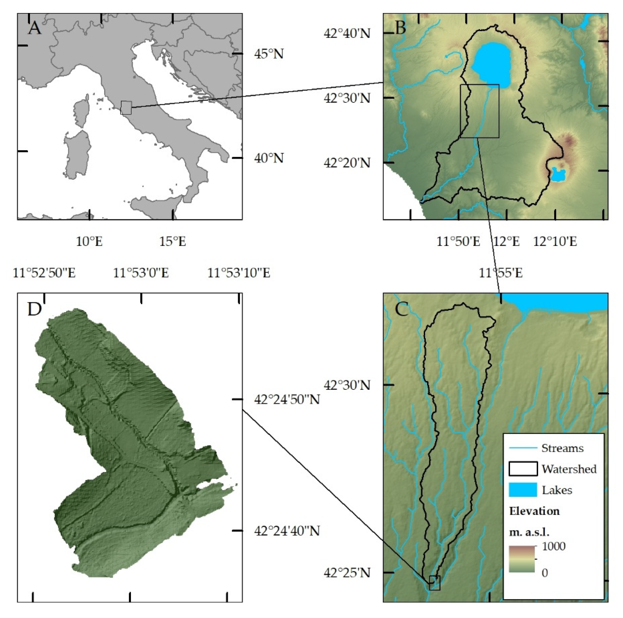
2.1. Case Study
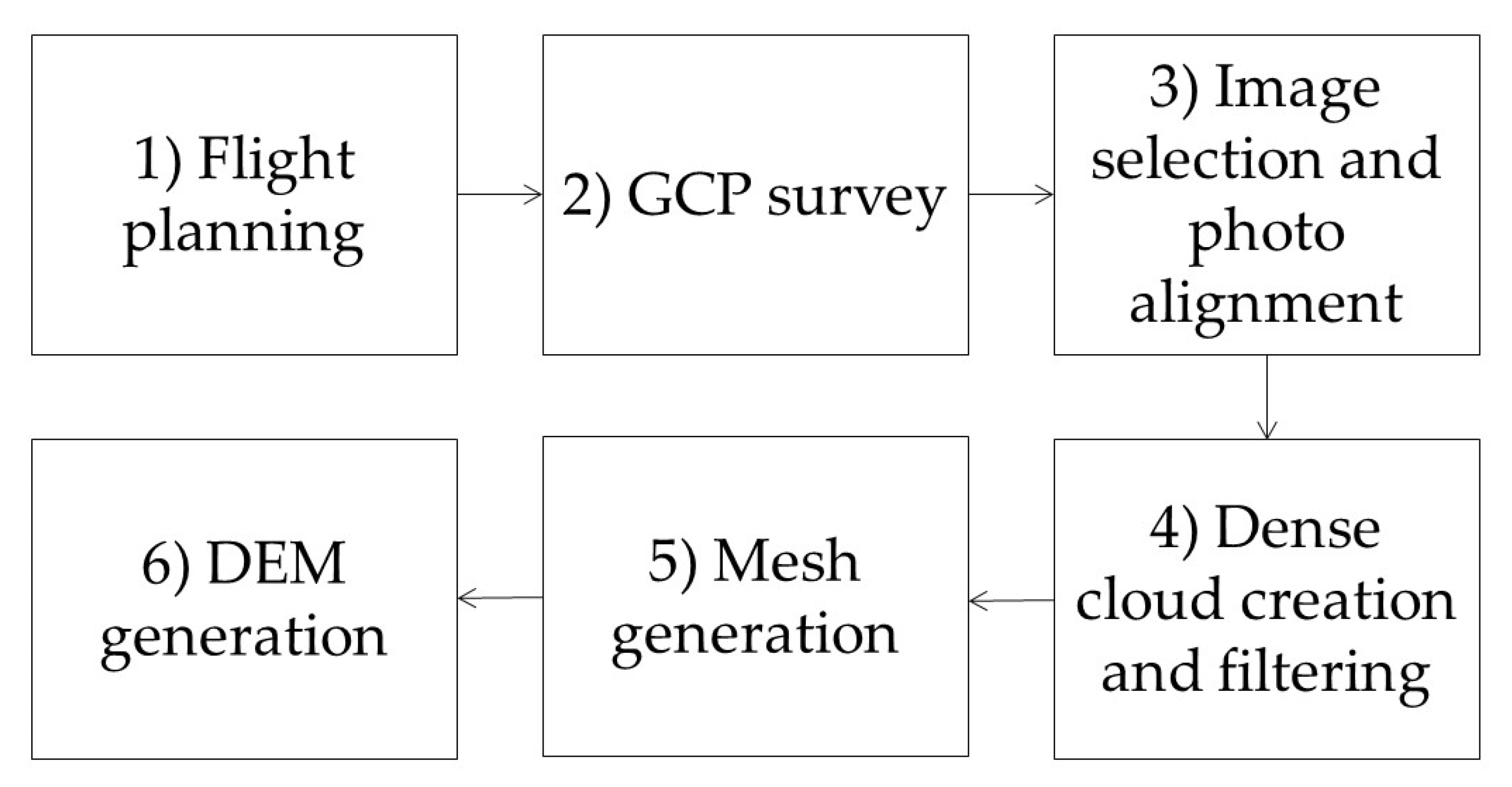
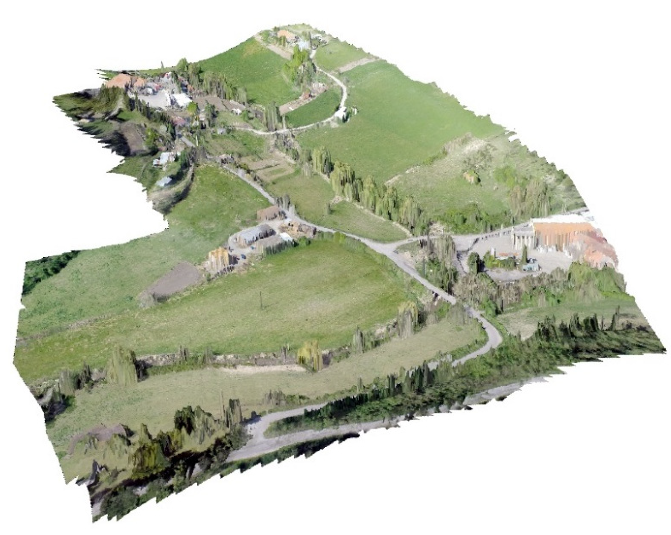
2.2. Topography and Digital Elevation Models
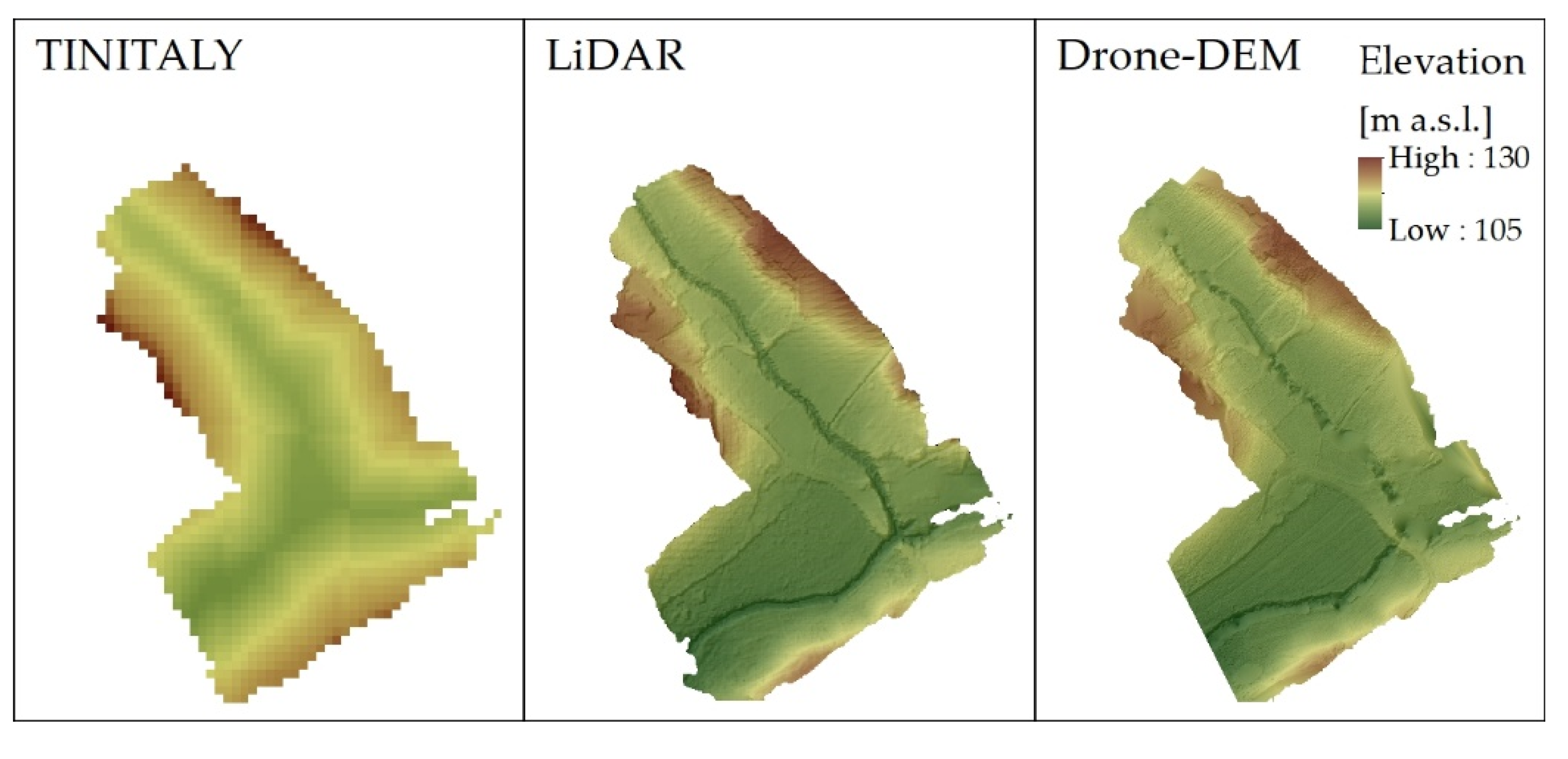
DEMs Comparison
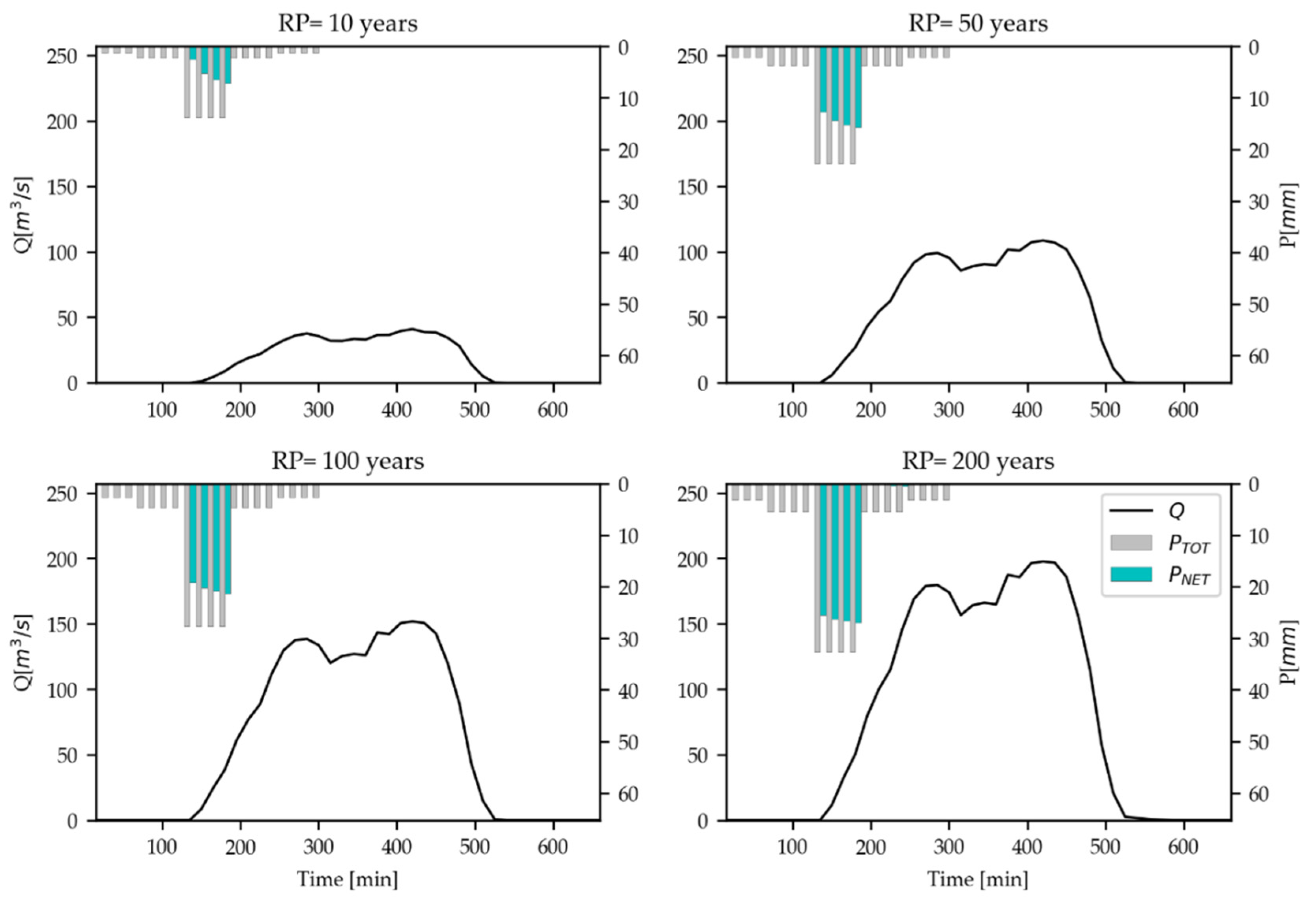
2.3. Hydrologic Modeling
2.4. Hydraulic Modeling
2.5. Inundation Extent Performance Indicators
3. Results
3.1. DEMs Comparison
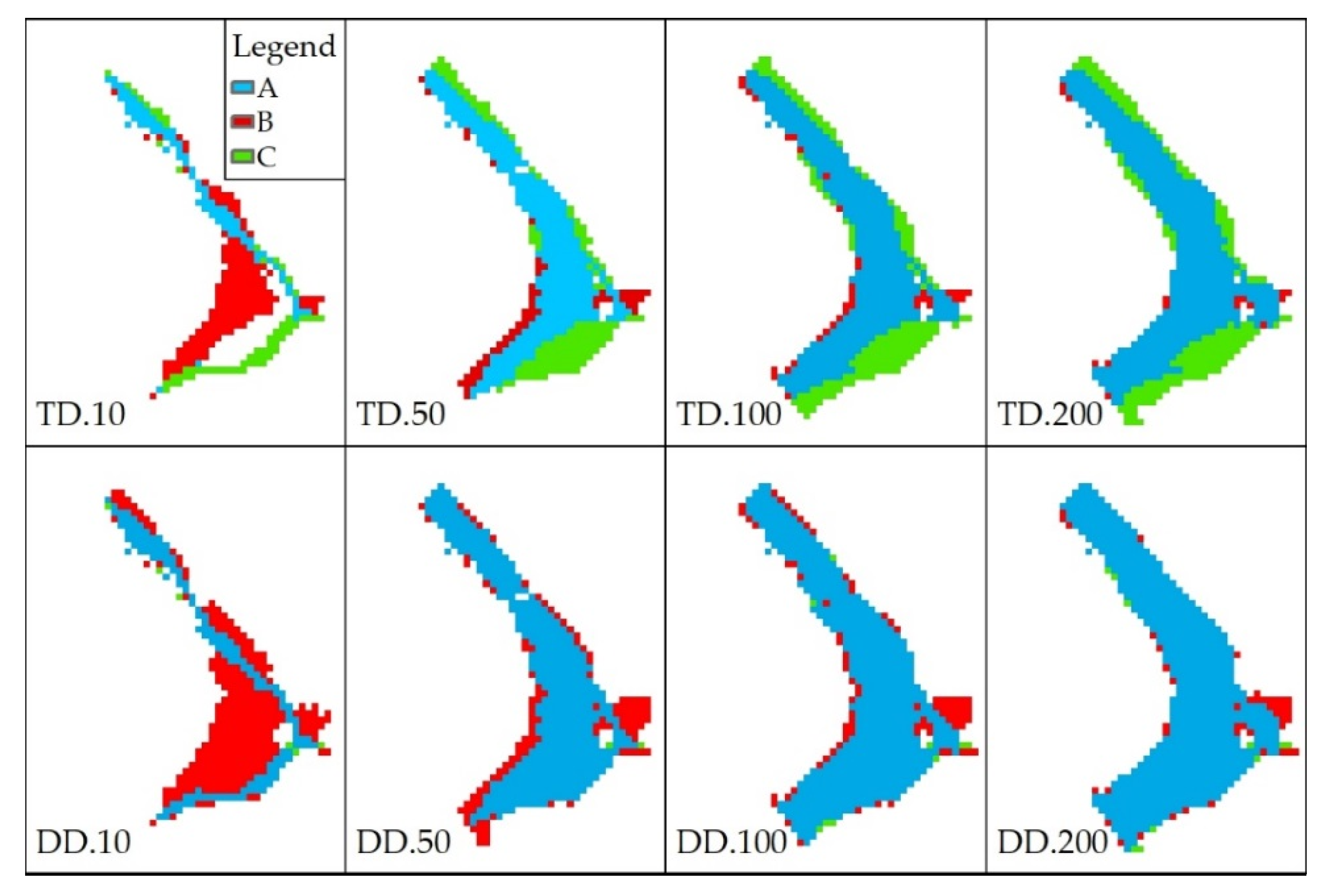
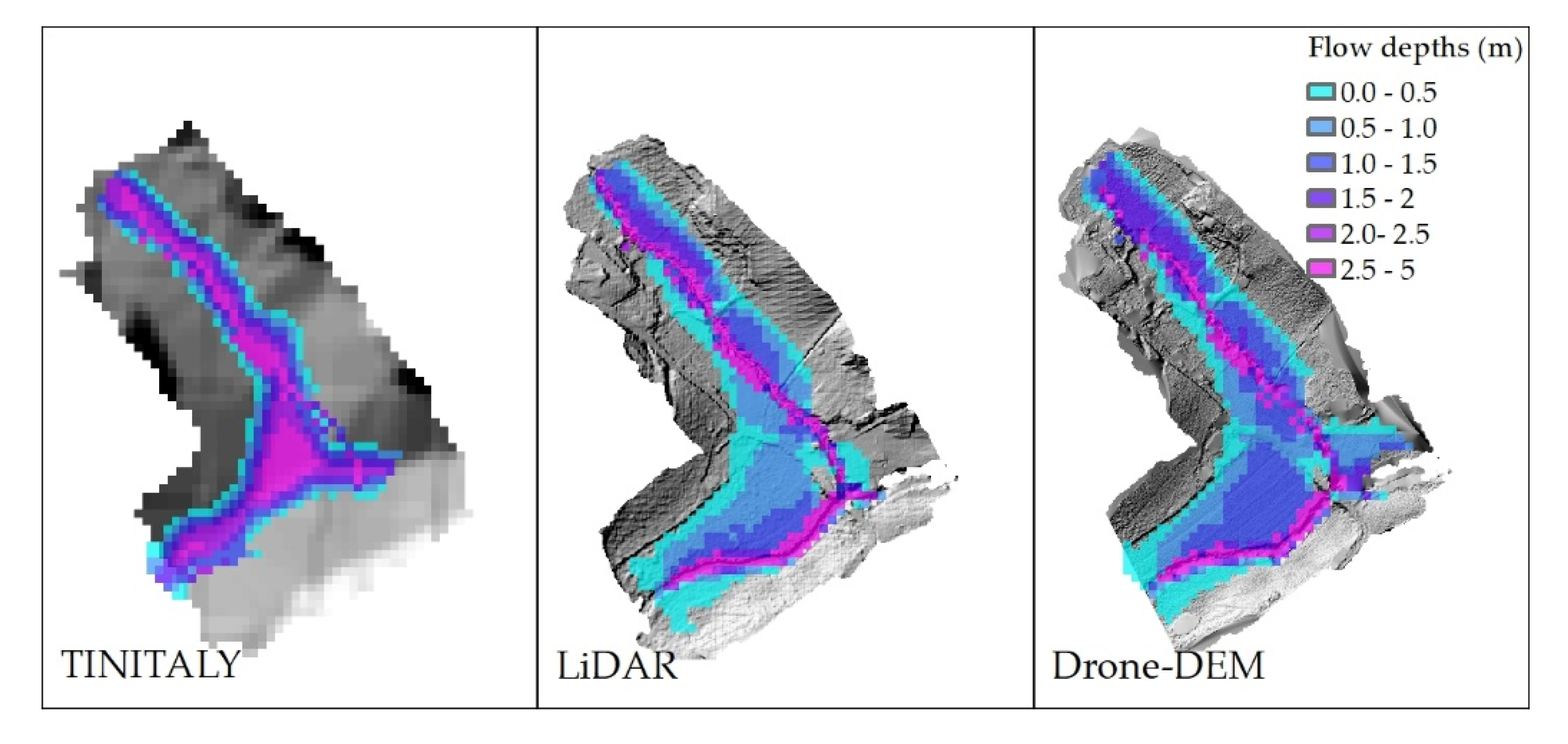
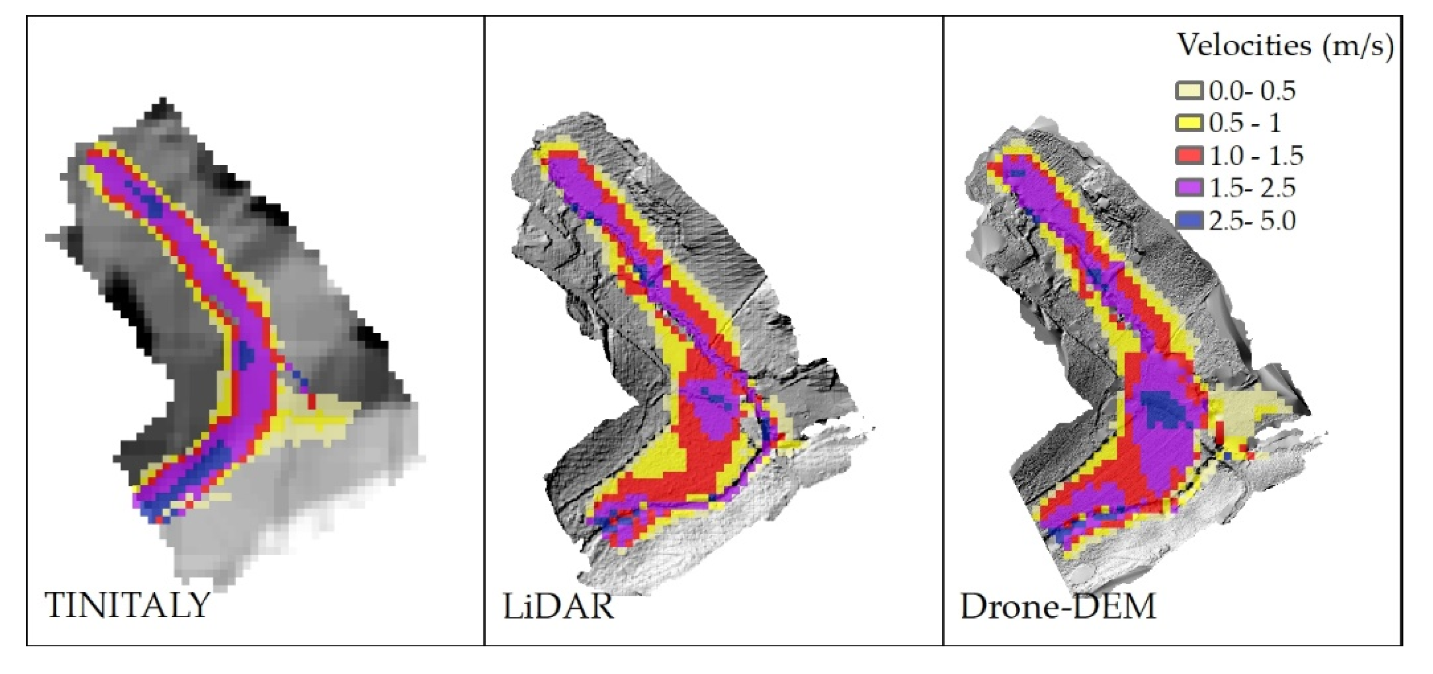
3.2. Inundation Modeling and Mapping Comparison
4. Discussion
5. Conclusions
Author Contributions
Funding
Acknowledgments
Conflicts of Interest
References
- Sampson, C.C.; Smith, A.M.; Bates, P.B.; Neal, J.C.; Alfieri, L.; Freer, J.E. A High-Resolution Global Flood Hazard Model. Water Resour. Res. 2015. [Google Scholar] [CrossRef] [PubMed]
- Dottori, F.; Salamon, P.; Bianchi, A.; Alfieri, L.; Hirpa, F.A.; Feyen, L. Development and Evaluation of a Framework for Global Flood Hazard Mapping. Adv. Water Resour. 2016, 94, 87–102. [Google Scholar] [CrossRef]
- Alfieri, L.; Bisselink, B.; Dottori, F.; Naumann, G.; Wyser, K.; Feyen, L.; De Roo, A. Global Projections of River Flood Risk in a Warmer World. Earth’s Future 2017. [Google Scholar] [CrossRef]
- Wing, O.E.J.; Bates, P.D.; Sampson, C.C.; Smith, A.M.; Johnson, K.A.; Erickson, T.A. Validation of a 30 m Resolution Flood Hazard Model of the Conterminous United States. Water Resour. Res. 2017, 53, 7968–7986. [Google Scholar] [CrossRef]
- Alfieri, L.; Burek, P.; Dutra, E.; Krzeminski, B.; Muraro, D.; Thielen, J.; Pappenberger, F. GloFAS-Global Ensemble Streamflow Forecasting and Flood Early Warning. Hydrol. Earth Syst. Sci. 2013. [Google Scholar] [CrossRef]
- Wu, H.; Adler, R.F.; Tian, Y.; Huffman, G.J.; Li, H.; Wang, J. Real-Time Global Flood Estimation Using Satellite-Based Precipitation and a Coupled Land Surface and Routing Model. Water Resour. Res. 2014. [Google Scholar] [CrossRef]
- Ward, P.J.; Jongman, B.; Salamon, P.; Simpson, A.; Bates, P.; De Groeve, T.; Muis, S.; De Perez, E.C.; Rudari, R.; Trigg, M.A.; et al. Usefulness and Limitations of Global Flood Risk Models. Nat. Clim. Chang. 2015. [Google Scholar] [CrossRef]
- Longuevergne, L.; Scanlon, B.R.; Wilson, C.R. GRACE Hydrological Estimates for Small Basins: Evaluating Processing Approaches on the High Plains Aquifer, USA. Water Resour. Res. 2010. [Google Scholar] [CrossRef]
- Grimaldi, S.; Petroselli, A. Do We Still Need the Rational Formula? An Alternative Empirical Procedure for Peak Discharge Estimation in Small and Ungauged Basins. Hydrol. Sci. J. 2015, 60, 67–77. [Google Scholar] [CrossRef]
- Blöschl, G.; Sivapalan, M.; Wagener, T.; Viglione, A.; Savenije, H. Runoff Prediction in Ungauged Basins: Synthesis across Processes, Places and Scales; Cambridge University Press: Cambridge, UK, 2013. [Google Scholar] [CrossRef]
- Ignacio, J.A.F.; Cruz, G.T.; Nardi, F.; Henry, S. Assessing the Effectiveness of a Social Vulnerability Index in Predicting Heterogeneity in the Impacts of Natural Hazards: Case Study of the Tropical Storm Washi Flood in the Philippines. Vienna Yearb. Popul. Res. 2015. [Google Scholar] [CrossRef]
- Convertino, M.; Annis, A.; Nardi, F. Information-Theoretic Portfolio Decision Model for Optimal Flood Management. Environ. Model. Softw. 2019, 119, 258–274. [Google Scholar] [CrossRef]
- McCabe, M.F.; Rodell, M.; Alsdorf, D.E.; Miralles, D.G.; Uijlenhoet, R.; Wagner, W.; Lucieer, A.; Houborg, R.; Verhoest, N.E.C.; Franz, T.E.; et al. The Future of Earth Observation in Hydrology. Hydrol. Earth Syst. Sci. 2017. [Google Scholar] [CrossRef] [PubMed]
- Tauro, F.; Selker, J.; Van De Giesen, N.; Abrate, T.; Uijlenhoet, R.; Porfiri, M.; Manfreda, S.; Caylor, K.; Moramarco, T.; Benveniste, J.; et al. Measurements and Observations in the XXI Century (MOXXI): Innovation and Multi-Disciplinarity to Sense the Hydrological Cycle. Hydrol. Sci. J. 2018. [Google Scholar] [CrossRef]
- Merwade, V.; Olivera, F.; Arabi, M.; Edleman, S. Uncertainty in Flood Inundation Mapping: Current Issues and Future Directions. J. Hydrol. Eng. 2008. [Google Scholar] [CrossRef]
- Grimaldi, S.; Petroselli, A.; Arcangeletti, E.; Nardi, F. Flood Mapping in Ungauged Basins Using Fully Continuous Hydrologic-Hydraulic Modeling. J. Hydrol. 2013. [Google Scholar] [CrossRef]
- Figorito, B.; Tarantino, E.; Balacco, G.; Fratino, U. An Object-Based Method for Mapping Ephemeral River Areas from WorldView-2 Satellite Data. In Remote Sensing for Agriculture, Ecosystems, and Hydrology XIV; SPIE: Bellingham, WA, USA, 2012. [Google Scholar] [CrossRef]
- Pappenberger, F.; Matgen, P.; Beven, K.J.; Henry, J.B.; Pfister, L.; Fraipont, P. Influence of Uncertain Boundary Conditions and Model Structure on Flood Inundation Predictions. Adv. Water Resour. 2006. [Google Scholar] [CrossRef]
- Apel, H.; Merz, B.; Thieken, A.H. Quantification of Uncertainties in Flood Risk Assessments. Int. J. River Basin Manag. 2008. [Google Scholar] [CrossRef]
- Bhuyian, M.N.M.; Kalyanapu, A.J.; Nardi, F. Approach to Digital Elevation Model Correction by Improving Channel Conveyance. J. Hydrol. Eng. 2015. [Google Scholar] [CrossRef]
- De Paola, F.; Giugni, M.; Pugliese, F.; Annis, A.; Nardi, F. GEV Parameter Estimation and Stationary vs. Non-Stationary Analysis of Extreme Rainfall in African Test Cities. Hydrology 2018, 5. [Google Scholar] [CrossRef]
- Nardi, F.; Annis, A.; Biscarini, C. On the Impact of Urbanization on Flood Hydrology of Small Ungauged Basins: The Case Study of the Tiber River Tributary Network within the City of Rome. J. Flood Risk Manag. 2018, 11, S594–S603. [Google Scholar] [CrossRef]
- Liu, Z.; Merwade, V.; Jafarzadegan, K. Investigating the Role of Model Structure and Surface Roughness in Generating Flood Inundation Extents Using One- and Two-Dimensional Hydraulic Models. J. Flood Risk Manag. 2019. [Google Scholar] [CrossRef]
- Petroselli, A.; Vojtek, M.; Vojteková, J. Flood Mapping in Small Ungauged Basins: A Comparison of Different Approaches for Two Case Studies in Slovakia. Hydrol. Res. 2019. [Google Scholar] [CrossRef]
- Peña, F.; Nardi, F. Floodplain Terrain Analysis for Coarse Resolution 2D Flood Modeling. Hydrology 2018. [Google Scholar] [CrossRef]
- Yan, K.; Di Baldassarre, G.; Solomatine, D.P.; Schumann, G.J.P. A Review of Low-Cost Space-Borne Data for Flood Modelling: Topography, Flood Extent and Water Level. Hydrol. Process. 2015. [Google Scholar] [CrossRef]
- Gioia, A.; Totaro, V.; Bonelli, R.; Esposito, A.A.M.G.; Balacco, G.; Iacobellis, V. Flood Susceptibility Evaluation on Ephemeral Streams of Southern Italy: A Case Study of Lama Balice. In Lecture Notes in Computer Science (including Subseries Lecture Notes in Artificial Intelligence and Lecture Notes in Bioinformatics); Springer: Cham, Switzerland, 2018. [Google Scholar] [CrossRef]
- Sammartano, G.; Spanò, A. DEM Generation Based on UAV Photogrammetry Data in Critical Areas. In Proceedings of the 2nd International Conference on Geographical Information Systems Theory, Applications and Management, Rome, Italy, 26–27 April 2016; pp. 92–98. [Google Scholar] [CrossRef]
- Polat, N.; Uysal, M. DTM Generation with UAV Based Photogrammetric Point Cloud. Int. Arch. Photogramm. Remote Sens. Spat. Inf. Sci.—ISPRS Arch. 2017, 42, 77–79. [Google Scholar] [CrossRef]
- Arif, F.; Abdul Maulud, K.N.; Ab Rahman, A.A. Generation of Digital Elevation Model through Aerial Technique. IOP Conf. Ser. Earth Environ. Sci. 2018, 169. [Google Scholar] [CrossRef]
- Manfreda, S.; McCabe, M.F.; Miller, P.E.; Lucas, R.; Madrigal, V.P.; Mallinis, G.; Dor, E.B.; Helman, D.; Estes, L.; Ciraolo, G.; et al. On the Use of Unmanned Aerial Systems for Environmental Monitoring. Remote Sens. 2018, 10. [Google Scholar] [CrossRef]
- Aguilar, F.J.; Rivas, J.R.; Nemmaoui, A.; Peñalver, A.; Aguilar, M.A. UAV-Based Digital Terrain Model Generation under Leaf-off Conditions to Support Teak Plantations Inventories in Tropical Dry Forests. A Case of the Coastal Region of Ecuador. Sensors (Switzerland) 2019, 19, 1934. [Google Scholar] [CrossRef]
- Pellicani, R.; Argentiero, I.; Manzari, P.; Spilotro, G.; Marzo, C.; Ermini, R.; Apollonio, C. UAV and Airborne LiDAR Data for Interpreting Kinematic Evolution of Landslide Movements: The Case Study of the Montescaglioso Landslide (Southern Italy). Geosciences 2019. [Google Scholar] [CrossRef]
- Fonstad, M.A.; Dietrich, J.T.; Courville, B.C.; Jensen, J.L.; Carbonneau, P.E. Topographic Structure from Motion: A New Development in Photogrammetric Measurement. Earth Surf. Process. Landf. 2013. [Google Scholar] [CrossRef]
- DeBell, L.; Anderson, K.; Brazier, R.E.; King, N.; Jones, L. Water Resource Management at Catchment Scales Using Lightweight UAVs: Current Capabilities and Future Perspectives. J. Unmanned Veh. Syst. 2016, 4, 7–30. [Google Scholar] [CrossRef]
- Kim, S.J.; Lim, G.J.; Cho, J. Drone Flight Scheduling under Uncertainty on Battery Duration and Air Temperature. Comput. Ind. Eng. 2018. [Google Scholar] [CrossRef]
- Nex, F.; Remondino, F. UAV for 3D Mapping Applications: A Review. Appl. Geomat. 2014. [Google Scholar] [CrossRef]
- Schumann, G.J.P.; Muhlhausen, J.; Andreadis, K.M. Rapid Mapping of Small-Scale River-Floodplain Environments Using UAV SfM Supports Classical Theory. Remote Sens. 2019, 11, 982. [Google Scholar] [CrossRef]
- Hashemi-Beni, L.; Jones, J.; Thompson, G.; Johnson, C.; Gebrehiwot, A. Challenges and Opportunities for UAV-Based Digital Elevation Model Generation for Flood-Risk Management: A Case of Princeville, North Carolina. Sensors 2018, 18, 3843. [Google Scholar] [CrossRef]
- Yao, H.; Qin, R.; Chen, X. Unmanned Aerial Vehicle for Remote Sensing Applications—A Review. Remote Sens. 2019. [Google Scholar] [CrossRef]
- Leitão, J.P.; Moy De Vitry, M.; Scheidegger, A.; Rieckermann, J. Assessing the Quality of Digital Elevation Models Obtained from Mini Unmanned Aerial Vehicles for Overland Flow Modelling in Urban Areas. Hydrol. Earth Syst. Sci. 2016, 20, 1637–1653. [Google Scholar] [CrossRef]
- Backes, D.; Schumann, G.; Teferele, F.N.; Boehm, J. Towards a High-Resolution Drone-Based 3D Mapping Dataset to Optimise Flood Hazard Modelling. Int. Arch. Photogramm. Remote Sens. Spat. Inf. Sci.—ISPRS Arch. 2019, 42, 181–187. [Google Scholar] [CrossRef]
- Mourato, S.; Fernandez, P.; Pereira, L.; Moreira, M. Improving a DSM Obtained by Unmanned Aerial Vehicles for Flood Modelling. IOP Conf. Ser. Earth Environ. Sci. 2017, 95. [Google Scholar] [CrossRef]
- Langhammer, J.; Bernsteinová, J.; Miřijovský, J. Building a High-Precision 2D Hydrodynamic Flood Model Using UAV Photogrammetry and Sensor Network Monitoring. Water 2017, 9, 861. [Google Scholar] [CrossRef]
- Watson, C.; Kargel, J.; Tiruwa, B. UAV-Derived Himalayan Topography: Hazard Assessments and Comparison with Global DEM Products. Drones 2019, 3, 18. [Google Scholar] [CrossRef]
- Sodnik, J.; Vrečko, A.; Podobnikar, T.; Mikoš, M. Digital Terrain Models and Mathematical Modelling of Debris Flows. Geod. Vestn. 2012. [Google Scholar] [CrossRef]
- Petroselli, A.; Grimaldi, S. Design Hydrograph Estimation in Small and Fully Ungauged Basins: A Preliminary Assessment of the EBA4SUB Framework. J. Flood Risk Manag. 2018, 11, S197–S210. [Google Scholar] [CrossRef]
- Grimaldi, S.; Petroselli, A.; Nardi, F. A Parsimonious Geomorphological Unit Hydrograph for Rainfall-Runoff Modelling in Small Ungauged Basins. Hydrol. Sci. J. 2012. [Google Scholar] [CrossRef]
- O’Brien, J.S.; Julien, P.Y.; Fullerton, W.T. Two-Dimensional Water Flood and Mudflow Simulation. J. Hydraul. Eng. 1993. [Google Scholar] [CrossRef]
- Tarquini, S.; Isola, I.; Favalli, M.; Mazzarini, F.; Bisson, M.; Pareschi, M.T.; Boschi, E. TINITALY/01: A New Triangular Irregular Network of Italy. Ann. Geophys. 2007. [Google Scholar] [CrossRef]
- Tarquini, S.; Vinci, S.; Favalli, M.; Doumaz, F.; Fornaciai, A.; Nannipieri, L. Release of a 10-m-Resolution DEM for the Italian Territory: Comparison with Global-Coverage DEMs and Anaglyph-Mode Exploration via the Web. Comput. Geosci. 2012. [Google Scholar] [CrossRef]
- Büttner, G.; Feranec, J.; Jaffrain, G.; Mari, L.; Maucha, G.; Soukup, T. The CORINE Land Cover 2000 Project. EARSeL eProceedings 2004, 3, 331–346. [Google Scholar]
- Scrinzi, G.; Floris, A.; Clementel, F.; Bernardini, V.; Chianucci, F.; Greco, S.; Michelini, T.; Penasa, A.; Puletti, N.; Rizzo, M.; et al. Models of Stand Volume and Biomass Estimation Based on LiDAR Data for the Main Forest Types in Calabria (Southern Italy). J. Silvic. For. Ecol. 2017. [Google Scholar] [CrossRef]
- Mason, D.C.; Cobby, D.M.; Horritt, M.S.; Bates, P.D. Floodplain Friction Parameterization in Two-Dimensional River Flood Models Using Vegetation Heights Derived from Airborne Scanning Laser Altimetry. Hydrol. Process. 2003, 17, 1711–1732. [Google Scholar] [CrossRef]
- Nardi, F.; Vivoni, E.R.; Grimaldi, S. Investigating a Floodplain Scaling Relation Using a Hydrogeomorphic Delineation Method. Water Resour. Res. 2006, 42. [Google Scholar] [CrossRef]
- Nardi, F.; Annis, A.; Di Baldassarre, G.; Vivoni, E.R.; Grimaldi, S. GFPLAIN250m, a Global High-Resolution Dataset of Earth’s Floodplains. Sci. Data 2019, 6, 1–6. [Google Scholar] [CrossRef] [PubMed]
- Dodov, B.; Foufoula-Georgiou, E. Generalized Hydraulic Geometry: Insights Based on Fluvial Instability Analysis and a Physical Model. Water Resour. Res. 2004. [Google Scholar] [CrossRef]
- Leopold, L.B.; Maddock, T.J. The Hydraulic Geometry of Stream Channels and Some Physiographic Implications; US Government Printing Office: Washington, WA, USA, 1953.
- Annis, A.; Nardi, F.; Morrison, R.R.; Castelli, F. Investigating Hydrogeomorphic Floodplain Mapping Performance with Varying DTM Resolution and Stream Order. Hydrol. Sci. J. 2019, 64, 525–538. [Google Scholar] [CrossRef]
- Nardi, F.; Morrison, R.R.; Annis, A.; Grantham, T.E. Hydrologic Scaling for Hydrogeomorphic Floodplain Mapping: Insights into Human-Induced Floodplain Disconnectivity. River Res. Appl. 2018, 34, 675–685. [Google Scholar] [CrossRef]
- Morrison, R.R.; Bray, E.; Nardi, F.; Annis, A.; Dong, Q. Spatial Relationships of Levees and Wetland Systems within Floodplains of the Wabash Basin, USA. J. Am. Water Resour. Assoc. 2018, 54, 934–948. [Google Scholar] [CrossRef]
- Scheel, K.; Morrison, R.R.; Annis, A.; Nardi, F. Understanding the Large-Scale Influence of Levees on Floodplain Connectivity Using a Hydrogeomorphic Approach. J. Am. Water Resour. Assoc. 2019, 55, 413–429. [Google Scholar] [CrossRef]
- Annis, A.; Nardi, F. Integrating VGI and 2D Hydraulic Models into a Data Assimilation Framework for Real Time Flood Forecasting and Mapping. Geo-Spat. Inf. Sci. 2019, 22, 223–236. [Google Scholar] [CrossRef]
- Hawker, L.; Neal, J.; Bates, P. Accuracy Assessment of the TanDEM-X 90 Digital Elevation Model for Selected Floodplain Sites. Remote Sens. Environ. 2019, 232. [Google Scholar] [CrossRef]
- Falorni, G.; Teles, V.; Vivoni, E.R.; Bras, R.L.; Amaratunga, K.S. Analysis and Characterization of the Vertical Accuracy of Digital Elevation Models from the Shuttle Radar Topography Mission. J. Geophys. Res. Earth Surf. 2005. [Google Scholar] [CrossRef]
- Piscopia, R.; Petroselli, A.; Grimaldi, S. A Software Package for Predicting Design-Flood Hydrographs in Small and Ungauged Basins. J. Agric. Eng. 2015, 46, 74–84. [Google Scholar] [CrossRef]
- Rossi, F.; Villani, P. A Project for Regional Analysis of Floods in Italy. In Coping with Floods; Springer: Dordrecht, The Netherlands, 1994. [Google Scholar] [CrossRef]
- Grimaldi, S.; Petroselli, A.; Romano, N. Green-Ampt Curve-Number Mixed Procedure as an Empirical Tool for Rainfall-Runoff Modelling in Small and Ungauged Basins. Hydrol. Process. 2013, 27, 1253–1264. [Google Scholar] [CrossRef]
- Grimaldi, S.; Petroselli, A.; Romano, N. Curve-Number/Green-Ampt Mixed Procedure for Streamflow Predictions in Ungauged Basins: Parameter Sensitivity Analysis. Hydrol. Process. 2013, 27, 1265–1275. [Google Scholar] [CrossRef]
- NRCS. National Engineering Handbook; NRCS: Washington, WA, USA, 1983.
- Nardi, F.; Grimaldi, S.; Santini, M.; Petroselli, A.; Ubertini, L. Hydrogeomorphic Properties of Simulated Drainage Patterns Using Digital Elevation Models: The Flat Area Issue. Hydrol. Sci. J. 2008. [Google Scholar] [CrossRef]
- Annis, A.; Nardi, F.; Volpi, E.; Fiori, A. Quantifying the Relative Impact of Hydrological and Hydraulic Modelling Parameterizations on Uncertainty of Inundation Maps. Hydrol. Sci. J. 2020, 65, 507–523. [Google Scholar] [CrossRef]
- Cobby, D.M.; Mason, D.C.; Davenport, I.J. Image Processing of Airborne Scanning Laser Altimetry Data for Improved River f Lood Modelling. ISPRS J. Photogramm. Remote Sens. 2001, 56, 121–138. [Google Scholar] [CrossRef]
- Apollonio, C.; Balacco, G.; Novelli, A.; Tarantino, E.; Piccinni, A.F. Land Use Change Impact on Flooding Areas: The Case Study of Cervaro Basin (Italy). Sustainability 2016. [Google Scholar] [CrossRef]
- Hooke, J.M. Variations in Flood Magnitude-Effect Relations and the Implications for Flood Risk Assessment and River Management. Geomorphology 2015. [Google Scholar] [CrossRef]
- Notti, D.; Giordan, D.; Caló, F.; Pepe, A.; Zucca, F.; Galve, J.P. Potential and Limitations of Open Satellite Data for Flood Mapping. Remote Sens. 2018. [Google Scholar] [CrossRef]
- Mason, D.C.; Horritt, M.S.; Hunter, N.M.; Bates, P.D. Use of Fused Airborne Scanning Laser Altimetry and Digital Map Data for Urban Flood Modelling. Hydrol. Process. 2007. [Google Scholar] [CrossRef]
- Pellicani, R.; Parisi, A.; Iemmolo, G.; Apollonio, C. Economic Risk Evaluation in Urban Flooding and Instability-Prone Areas: The Case Study of San Giovanni Rotondo (Southern Italy). Geosciences 2018. [Google Scholar] [CrossRef]
- Dottori, F.; Di Baldassarre, G.; Todini, E. Detailed Data Is Welcome, but with a Pinch of Salt: Accuracy, Precision, and Uncertainty in Flood Inundation Modeling. Water Resour. Res. 2013. [Google Scholar] [CrossRef]
- Ferrari, A.; Viero, D.P.; Vacondio, R.; Defina, A.; Mignosa, P. Flood Inundation Modeling in Urbanized Areas: A Mesh-Independent Porosity Approach with Anisotropic Friction. Adv. Water Resour. 2019. [Google Scholar] [CrossRef]
- Miller, J.D.; Hutchins, M. The Impacts of Urbanisation and Climate Change on Urban Flooding and Urban Water Quality: A Review of the Evidence Concerning the United Kingdom. J. Hydrol. Reg. Stud. 2017. [Google Scholar] [CrossRef]


| DEM | Resolution (m) | Coverage | Cost (€/km2) | Vertical Accuracy (m) | Year |
|---|---|---|---|---|---|
| TINITALY | 10 | Entire country | Free | ±16 [50,51] | 2007 |
| LiDAR | 1 | Major rivers/coasts | 1000–5000 1 | ±0.15–0.30 [53] | 2011 |
| Drone 3 | 0.25 | Local scale | 500–1500 2 | ±0.10 | 2015 |
| DEM | MD (m) | RMSD (m) | STD (m) | Skew (−) |
|---|---|---|---|---|
| TINITALY | −5.76 | 6.10 | 2.01 | −0.89 |
| Drone-DEM | −0.05 | 0.75 | 0.75 | −4.44 |
| Return Period (Years) | DEM | TP | FP | CSI |
|---|---|---|---|---|
| 10 | TINITALY | 0.57 | 0.66 | 0.27 |
| Drone-DEM | 0.96 | 0.67 | 0.32 | |
| 50 | TINITALY | 0.70 | 0.16 | 0.62 |
| Drone-DEM | 1.00 | 0.21 | 0.79 | |
| 100 | TINITALY | 0.71 | 0.09 | 0.66 |
| Drone-DEM | 0.98 | 0.13 | 0.86 | |
| 200 | TINITALY | 0.72 | 0.03 | 0.71 |
| Drone-DEM | 0.98 | 0.07 | 0.92 |
| Return Period (Years) | DEM | MD | RMSD | STD |
|---|---|---|---|---|
| 10 | TINITALY | 0.01 | 0.42 | 0.42 |
| Drone-DEM | −0.13 | 0.56 | 0.55 | |
| 50 | TINITALY | −0.49 | 1.11 | 1.00 |
| Drone-DEM | −0.11 | 0.49 | 0.48 | |
| 100 | TINITALY | −0.45 | 1.13 | 1.04 |
| Drone-DEM | −0.04 | 0.46 | 0.46 | |
| 200 | TINITALY | −0.42 | 1.14 | 1.06 |
| Drone-DEM | −0.02 | 0.46 | 0.46 |
© 2020 by the authors. Licensee MDPI, Basel, Switzerland. This article is an open access article distributed under the terms and conditions of the Creative Commons Attribution (CC BY) license (http://creativecommons.org/licenses/by/4.0/).
Share and Cite
Annis, A.; Nardi, F.; Petroselli, A.; Apollonio, C.; Arcangeletti, E.; Tauro, F.; Belli, C.; Bianconi, R.; Grimaldi, S. UAV-DEMs for Small-Scale Flood Hazard Mapping. Water 2020, 12, 1717. https://doi.org/10.3390/w12061717
Annis A, Nardi F, Petroselli A, Apollonio C, Arcangeletti E, Tauro F, Belli C, Bianconi R, Grimaldi S. UAV-DEMs for Small-Scale Flood Hazard Mapping. Water. 2020; 12(6):1717. https://doi.org/10.3390/w12061717
Chicago/Turabian StyleAnnis, Antonio, Fernando Nardi, Andrea Petroselli, Ciro Apollonio, Ettore Arcangeletti, Flavia Tauro, Claudio Belli, Roberto Bianconi, and Salvatore Grimaldi. 2020. "UAV-DEMs for Small-Scale Flood Hazard Mapping" Water 12, no. 6: 1717. https://doi.org/10.3390/w12061717
APA StyleAnnis, A., Nardi, F., Petroselli, A., Apollonio, C., Arcangeletti, E., Tauro, F., Belli, C., Bianconi, R., & Grimaldi, S. (2020). UAV-DEMs for Small-Scale Flood Hazard Mapping. Water, 12(6), 1717. https://doi.org/10.3390/w12061717