Effects of Land Use Changes on Streamflow and Sediment Yield in Atibaia River Basin—SP, Brazil

Abstract

The Soil and Water Assessment Tool (SWAT) is often used to evaluate the impacts of different land use scenarios on streamflow and sediment yield, but there is a need for some clear recommendations on how to select the parameter set that defines a given land use scenario and on what is the most appropriate methodology to change the selected parameters when describing possible future conditions. This paper reviews the SWAT formulation to identify the parameters that depend on the land use, performs a sensitivity analysis to determine the ones with larger impacts on the model results and discusses ways to consider future land use conditions. The case study is the Atibaia river basin, with 2838 km² (São Paulo, Brazil). The parameters identified by sensitivity analysis with the largest impacts on streamflow and sediment yield were the initial curve number for moisture condition II (CN), maximum canopy storage for each land use (CANMX) and the cover and management factor (USLE_C). The identification and appropriate parameter change can provide real estimates of the magnitudes in the land use changes, which were verified in this study. Such information can be used as an instrument for proposing improvements in the basin’s environmental quality and management.

1. Introduction

Understanding the implications of land use change is critical to the river basin planning and remediation efforts that are occurring all over the globe. The impacts of land use modification on river hydrological behavior need to be evaluated when reviewing current and future water availability, assessing river basin degradation processes or identifying the most appropriate measures to control the impacts caused by the disorderly land use change [1,2,3].

The effects of land use changes are empirically known but it is often very difficult to explicitly quantify them [3]. Geographic information system (GIS) and distributed hydrological models may contribute to overcome this challenge [4].

By offering the possibility to assess the behavior of a watershed under different scenarios, hydrological models may be used to predict the consequences of land use changes on the simulated hydrological processes [5]. The Soil Water Assessment Tool (SWAT) [6,7] is the focus of the paper, given its popularity for land use impacts assessment and because its formulation is based on physical parameters, most of which can in theory be measured in the field, therefore facilitating the description of different land use situations. Other popular hydrology models that may be used to assess land use changes include the Hydrologic Modeling System (HEC-HMS) [8] and the Geospatial Streamflow Model-GeoSFM model [9].

Many authors have used SWAT to evaluate the impacts of land use change [3,10,11,12,13,14]. Unfortunately, there is a lack of consensus on how to apply the model for this purpose, namely, determining which set of model parameters is related to land use, how the model should be calibrated and validated for a reference land use condition and how the parameters should be changed in a consistent way to reflect a modified land use condition land use scenario.

Most studies cite the Soil Conservation Service (SCS) curve number (CN) as the most important land use related parameter, together with the Maximum Canopy Storage (CANMX) and the Leaf Area Index (LAI). The soil cover parameter C of the Universal Soil Loss Equation (USLE) is also considered when evaluating the impacts on erosion yield. However, SWAT has a few other parameters also related to soil cover and soil use which are required to be evaluated if changes of their values do not affect the model results.

Furthermore, when calibrating SWAT for a certain land use condition, model parameters, including land use related ones, are modified so that model results reproduce streamflow and sediment yield measured values. Following calibration, it is not clear how model parameters should be further modified to reflect a change of land use in the river basin. Moreover, as these parameter modifications can be inserted in SWAT in different ways, there is a need for recommendations on how to do it in a consistent way.

Therefore, the main objective of the present research is to study how SWAT should be used to assess the impacts of land use changes on streamflow and sediment yield. The model formulation is analyzed to identify all the parameters that are related to land use, and a sensitivity analysis is performed to determine the most important ones. Some recommendations are put forward on how to use these parameters, in a consistent way and following the model calibration and validation, when representing new land use scenarios.

The case study is the Atibaia river basin located in the interior of São Paulo state, Brazil, which is experiencing important land use changes. The growth of agricultural activity in the last decades, has led to conversion of pastures into agricultural land, mostly for sugar cane production, and to a degradation process with significant environmental impacts [15,16]. The current study adds to existing studies that have identified the environmental impacts of this deforestation trend [15,16,17,18], by quantifying the impacts on streamflow and sediment yield in the river basins with significant agricultural areas.

2. Methodology

2.1. SWAT Model

SWAT is a semi-distributed model which uses meteorological data, elevation data, soil types and land use to calculate the daily water, sediments and contaminants balance of a river basin [7]. The river basin is partitioned into sub-basins and hydrological response units (HRUs), with each HRU corresponding to a single combination of land use, soil type, slope and management practices.

The model assumes a division of the lithological profile into three zones: the vadose zone, the shallow aquifer, and the deep aquifer, with only the two upper ones contributing to the river streamflow. Water and contaminants percolating into the lower one are removed from the basin daily balance [19].

The model simulates the water flow through the river basin, including its land phase over the terrain and through the soil and its water phase in the river channels. Along the way, water erodes, carries and deposits sediments, nutrients, pesticides and other contaminants and controls plant growth [7,20,21].

Table 1. Soil Water Assessment Tool (SWAT) components.

SWAT Components	Description
Hydrology	Four main processes are considered: runoff, evapotranspiration, soil water movement and groundwater. All of these processes are accounted for in the model’s water balance equation.
Weather	Climate is the main process inducing agent of the terrestrial phase of the hydrological cycle. The model requires daily data and monthly data of various meteorological variables.
Erosion/Sedimentation	Sediment yield is calculated for each HRU using the Modified Universal Soil Loss Equation. Vegetation cover and crop residues are considered when estimating soil particles detachment and transport.
Land use and Plant growth	Plant growth is simulated using an Erosion Productivity Impact Calculator (EPIC) simplification and occurs only on days when the average daily temperature exceeds a plant-specific base temperature [22].
Nutrients and Pesticides	Nitrogen and phosphorus movement and transformation is traced within the basin. In addition, pesticide loading, and bacterial contamination can also be computed.
Management practices	Crop cultivation, growth and grazing are simulated, as well as irrigation and nutrient and pesticide applications. Soil protection offered by vegetation throughout the year and the deposition of crop remains on the soil after harvest is considered.
Main channel processes	The movement of water, sediment, nutrients, and pesticides through the channel is computed. The channel dimensions are usually assumed constant, but there is an option to assume them dependent on erosion and deposition.
Water bodies	In addition to channels, water may flow through four types of water bodies: ponds, wetlands, depressions, and reservoirs.

presents and describes the 8 main components of SWAT.

This study used SWAT 2012, released on 2018, integrating an ArcView GIS interface.

2.2. SWAT Land Use Parameters

Most studies found in the literature cite CN as the most important parameter of the SWAT model related to land use, which is used to calculate the runoff volume and infiltration. CN values range between 0 and 100, with higher CN values associated with areas with higher runoff potential such as urban districts. Low values indicate large retention and soil infiltration capacity and low runoff potential, occurring for example in forest areas [7,23].

The CN parameter is variable for each HRU and is computed from the combination of the hydrologic soil group and land use [24]. The combination table proposed by the SCS is stored in the model database and when new land use maps are loaded to the model, the model automatically determines new CN values for each HRU. Land use maps may be obtained from satellite images [10,11,12,13,14,25] or from hypothetically designed maps to predict possible future changes [3,26,27].

Local CN values change from event to event due to antecedent moisture conditions, as SWAT adjusts the daily CN according to the retention parameter that varies with soil profile water content or with accumulated plant evapotranspiration. We have decided to adjust CN according to the plant evapotranspiration because the alternative often results in over prediction of runoff in shallow soils. By calculating daily CN as a function of plant evapotranspiration, the value is less dependent on soil storage and more dependent on antecedent climate [28,29].

During model calibration and validation, CN values can be changed by directly altering the SCS original table, but this is usually not done. Alternatively, the database values are multiplied by an HRU dependent percentage change value, therefore ensuring the relative physical meaning of CN for different soils or HRUs [30].

The maximum canopy storage (CANMX) parameter is also mentioned by several studies as important in simulating the impacts of land use changes in the streamflow [12,13,31]. The CANMX is the maximum amount of water that can be stored in the canopy and trunks of fully developed trees [31]. Its value controls the density of plant cover so that it significantly affects infiltration and evapotranspiration.

A CANMX value is defined for each crop and a first estimate is stored in the model database. The canopy storage in each day depends on the leaf area index of the specific crop [7] (Equation (1)):

$$CANM{X}_{day}=CANMX\times \raisebox{1ex}{$LAI$}\!\left/ \!\raisebox{-1ex}{$LA{I}_{mx}$}\right.$$

(1)

where $CANM{X}_{day}$ is the canopy storage at day t (mm), LAI is the leaf area index and LAI_mx the maximum leaf area index. $LAI$ increases until the maximum leaf area index ($LA{I}_{mx}$) is achieved, then remains constant until onset of senescence, after which it declines to zero at harvest [32].

The LAI represents the structural properties of the plant canopy and impacts the exchange of energy and mass fluxes between the surface and the atmospheric boundary layer [33,34,35].

SWAT estimates LAI from the canopy height, $h_c$ (cm), the fraction of the plant’s maximum leaf area index, $f{r}_{LAImx}$ and the fraction of potential heat units accumulated for the plant on a given day in the growing season, $f{r}_{PHU}$ [36]. The fraction of potential heat units accumulated by a given day is calculated from the heat unit accumulated on day i (heat units), HU, and the total heat units required for plant maturity (heat units), PHU. Heat units are calculated from maximum and minimum air temperature and from the plant-specific base temperature. No growth occurs for average temperatures at or below the crop base temperature [7,19].

The values of the parameters describing the behavior of each crop, such as $LA{I}_{mx}$, $h_{c,mx}$ and PHU, are stored in the model database. This database can be added or changed if different crops must be considered or if there is information particular to the study area, but usually the crop specific parameters are not changed during model calibration. The value of the maximum canopy storage (CANMX) can however be changed and defined as a function of the soil cover. The values have been obtained and adapted from literature recommending CANMX value for different land uses [37,38].

The erosion/sedimentation sub model of SWAT uses the Modified Universal Soil Loss Equation (MUSLE) method [39] to determine soil erosion and sediment yield from each HRU. The simulation of the impacts of land use changes on sediment yield can be studied by changing the USLE C parameter, which reflects the protection given to the soil by surface cover [40,41]. High values of USLE_C represent landscape management practices that need to be improved, while lower values demonstrate that the management practices used are environmentally favorable, as is the case in forest areas [7,42,43].

SWAT updates USLE_C daily (Equation (2)) as plant cover varies during the growth cycle of the plant [7]:

$$USLE\_C_{day}=\exp \left(\left[ln\left(0.8\right)-ln\left(USLE\_C\right)\right]·exp\left[-0.00115·rs{d}_{surf}\right]+ln\left(USLE\_C\right)\right)$$

(2)

$USLE\_C_{day}$ is the value for the cover and management factor for the land cover updates daily computed by SWAT; $USLE\_C$ is the value for the cover and management factor for the land cover given by the user; and $rs{d}_{surf}$ is the amount of residue on the soil surface (kg/ha) contained on the top 10mm of soil, which depends on weather conditions such as precipitation, temperature, solar radiation, humidity and wind speed [44].

SWAT assigns default values for the cover and management factor for each crop, however these values were not consistent with the reality of the study area located in Brazil. The values of the USLE_C were assigned manually, based on studies carried out in the study region [36,45,46,47].

2.3. Model Calibration and Validation

The model calibration and validation were conducted using the available data (1987–2015). The first 3 years of the record (1987–1989) were used to warm up the model; a second period (1990–2003) was used to calibrate it; and the final period (2004–2015) to validate the calibration.

The quantity of parameters of SWAT hinders the possibility of manually calibrating all the parameters. Therefore, the calibration proceeded in three stages. First, a literature review identified the parameters most likely to significantly affect the model results [19,28,48,49,50,51,52,53,54]. Further, the sequential uncertainty fitting method (SUFI2), within SWAT-CUP, was processed to identify the parameters to which the model results are most sensitive. Finally, a manual calibration of those parameters was accomplished trying to improve the fit between the results simulated by the model and observed flow values.

SWAT performance was assessed using the following indicators: Nash and Sutcliffe efficiency [55], the percent bias (Pbias), and the coefficient of determination (r2).

The Nash and Sutcliffe efficiency (NSE) evaluates a normalized difference between the model results and the observed results (Equation (3)):

$$\mathrm{NSE}=1-\left(\frac{\sum {\left({\mathrm{Y}}_{\mathrm{t}}^{\mathrm{obs}}-{\mathrm{Y}}_{\mathrm{t}}^{\mathrm{sim}}\right)}^2}{\sum {\left({\mathrm{Y}}_{\mathrm{t}}^{\mathrm{obs}}-\overline{{\mathrm{Y}}_{\mathrm{t}}^{\mathrm{obs}}}\right)}^2}\right)$$

(3)

where ${\mathrm{Y}}_{\mathrm{t}}^{\mathrm{obs}}$ is the observed value, $\overline{{\mathrm{Y}}_{\mathrm{t}}^{\mathrm{obs}}}$ is the average observed value, ${\mathrm{Y}}_{\mathrm{t}}^{\mathrm{sim}}$ is the computed value, $\overline{{\mathrm{Y}}_{\mathrm{t}}^{\mathrm{sim}}}$ is the average computed value. The NSE values ranges between −∞ and the optimal value of 1, with values less than 0 indicating that it is better to use the observed average than the values predicted by the model (Moriasi, 2007).

The percent of Pbias (PBIAS) indicates the average tendency of the simulated flows to be higher or lower than the observed flow, with values close to zero indicating a good adjustment of the simulated results to the observed data (Equation (4)):

$${\mathrm{P}}_{\mathrm{BIAS}}=\left(\frac{\sum {\mathrm{Y}}_{\mathrm{t}}^{\mathrm{obs}}-\sum {\mathrm{Y}}_{\mathrm{t}}^{\mathrm{sim}}}{\sum {\mathrm{T}}_{\mathrm{t}}^{\mathrm{obs}}}\right)·100$$

(4)

The coefficient of determination (r2) represents the proportion of the observed data variance that is explained by the model. The coefficient ranges between 0 and 1, with higher values representing a better performance of the model and less variation in the error [56].

$$r^2=\frac{{(\sum \left[Y_t^{obs}-\overline{Y_t^{obs}}\right]\left[Y_t^{sim}-\overline{Y_t^{sim}}\right])}^2}{\sum {\left(Y_t^{obs}-\overline{Y_t^{obs}}\right)}^2\sum {\left(Y_t^{sim}-\overline{Y_t^{sim}}\right)}^2}$$

(5)

2.4. Land Use Scenario Simulation

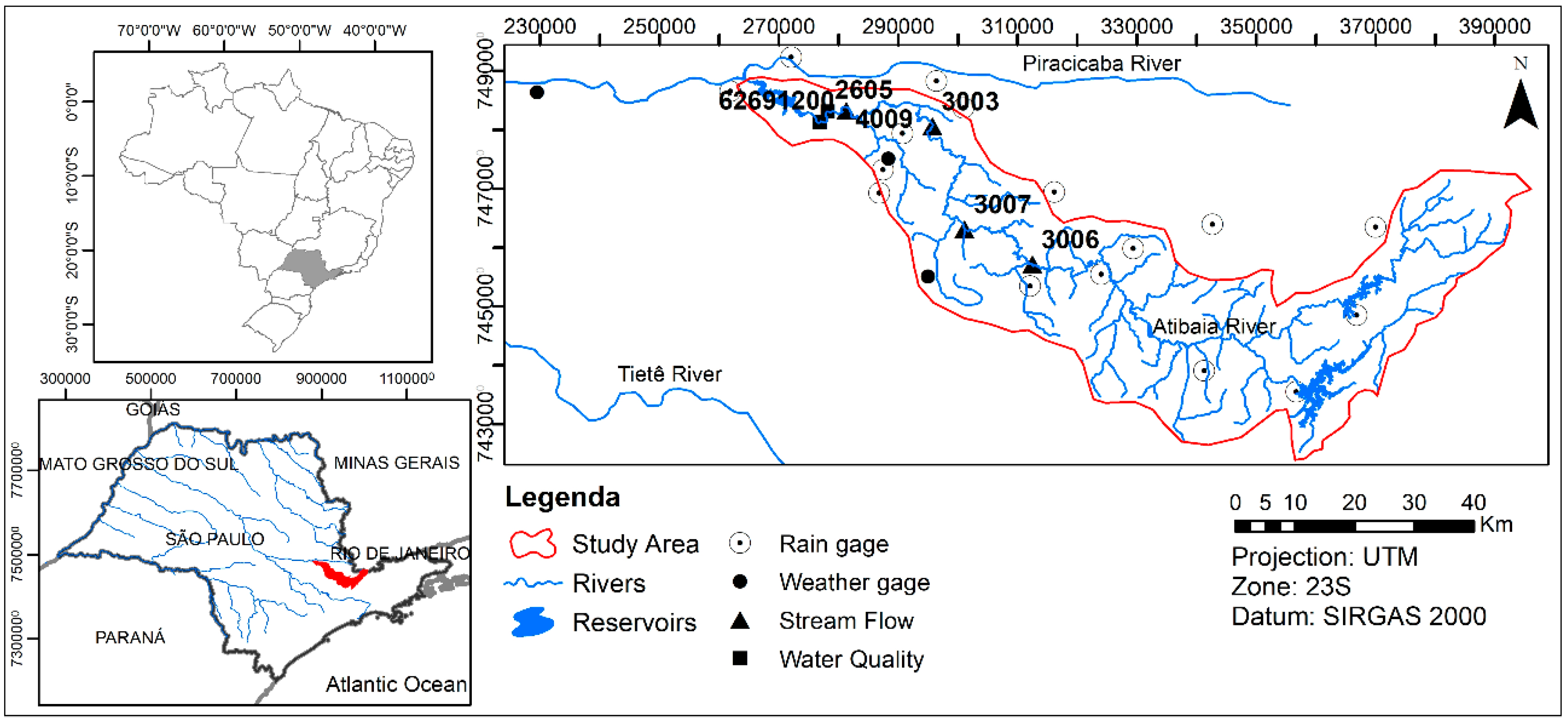
Land use change impacts on streamflow were evaluated by importing each land use scenario, and new land use maps were imported into SWAT. As CN, CANMX and USLE_C were setup to be solely dependent on land use, their values were automatically updated by the model.

3. Study Area

3.1. Watershed Data

The Atibaia river basin has an area of 2837.3 km², covering several municipalities of São Paulo and Minas Gerais states (Figure 1). According to [57], the total population of the basin is approximately 372,456 habitants, served mostly from surface water sources.

The watershed altitude ranges from 509 m, in the West, to 2029 m, in the East. A 12.5 m resolution DEM, obtained from Advanced Land Observing Satellite–ALOS, was used to describe topography.

Currently, the river basin rural areas are mainly covered by pastures, sugar cane and mixed forests. In recent decades, agriculture activity has been growing, with and intensification of land use and the substitution of perennial and semi-perennial agriculture (pasture, orange, corn, coffee, etc) mainly by sugarcane [15,16].

The soil map was obtained at EMBRAPA (Empresa Brasileira de Pesquisa Agropecuária). It recognizes three major soil types in the basin: red-yellow latosol (covering 61.01% of the river basin area), typic haplortox (37.75%) and typic eutrorthox (1.24%). The parameter values describing the soil characteristics were acquired from [58,59,60,61].

The Lower Atibaia sub-basin has conditions of geology, pedology and slope that favors infiltration, namely thick soil profiles (>20 m) of sandy texture and low compactness. The Intermediate/Lower Atibaia sub-basin local conditions result in thinner alteration profiles (10 to 20 m) in slabby terrain and shallow profiles (<5 m) in the steeper parts of the basin. The Intermediate/Upper Atibaia sub-basin has thin soils (up to 5m), of medium to fine texture and low consistency with less noticeable infiltration conditions. The Upper Atibaia sub-basin has shallow soil profiles (<2 m thick) of fine texture and medium consistency, with limited infiltration conditions.

The hydrometric data were obtained from the databases of two government agencies: ANA (Agência Nacional de Águas) and DAEE (Departamento de Águas e Energia do Estado de São Paulo). Four hydrographic gages (4009, 3003, 3006 and 3007) and 17 rain gages (Figure 1) were selected due to their location and data completeness. Data on temperature, humidity, wind speed and solar radiation was obtained from a weather gage located near to the basin and operated by ESALQ (Escola Superior de Agricultura Luiz de Queiroz).

Atibaia river basin can be divided into four units. The Lower Atibaia sub-basin (hydrograph gage 4009) with 349 km², the Intermediate Lower Atibaia sub-basin (hydrograph gage 3003), with 333 km², the Intermediate Upper Atibaia sub-basin (hydrograph gage 3007), 233 km², and the Upper Atibaia sub-basin (hydrograph gage 3006), with 1923 km².

The basin main land uses are pasture, natural vegetation (seasonal semi-deciduous forest), and agricultural crops, such as orange, coffee, corn, soy, and sugarcane, followed by urban areas, reforestation areas (eucalyptus) and water bodies [62,63]. From 1990 to 2016, various crops such as coffee and oranges have been replaced by sugar cane, due to the great economic incentive for ethanol production.

The Lower Atibaia sub-basin is covered with mixed forest (16.96% of the river basin area), pasture (20.67%), urban area (36.43%), agriculture (4.11%), range-grasses (7.14%), water (4.41%), sugarcane (10.11%) and mineral transportation (0.17%). The Intermediate Lower Atibaia sub-basin is covered with mixed forest (34.19% of the river basin area), pasture (30.05%), urban area (29.90%), agriculture (2.67%), range-grasses (1.82%), water (0.90%), sugarcane (0.40%) and mineral transportation (0.08%). The Intermediate Upper Atibaia sub-basin is coved with mixed forest (35.87% of the river basin area), pasture (39.47%), urban area (14.76%), agriculture (4.38%), range-grasses (3.80%), water (0.83%) and sugarcane (0.88%). Finally, in the Upper Atibaia sub-basin the uses are mixed forests (50.89% of the river basin area), pasture (29.45%), urban area (11.55%), agriculture (3.83%), range-grasses (2.40%), water (1.77%), sugarcane (0.10%) and mineral transportation (0.01%).

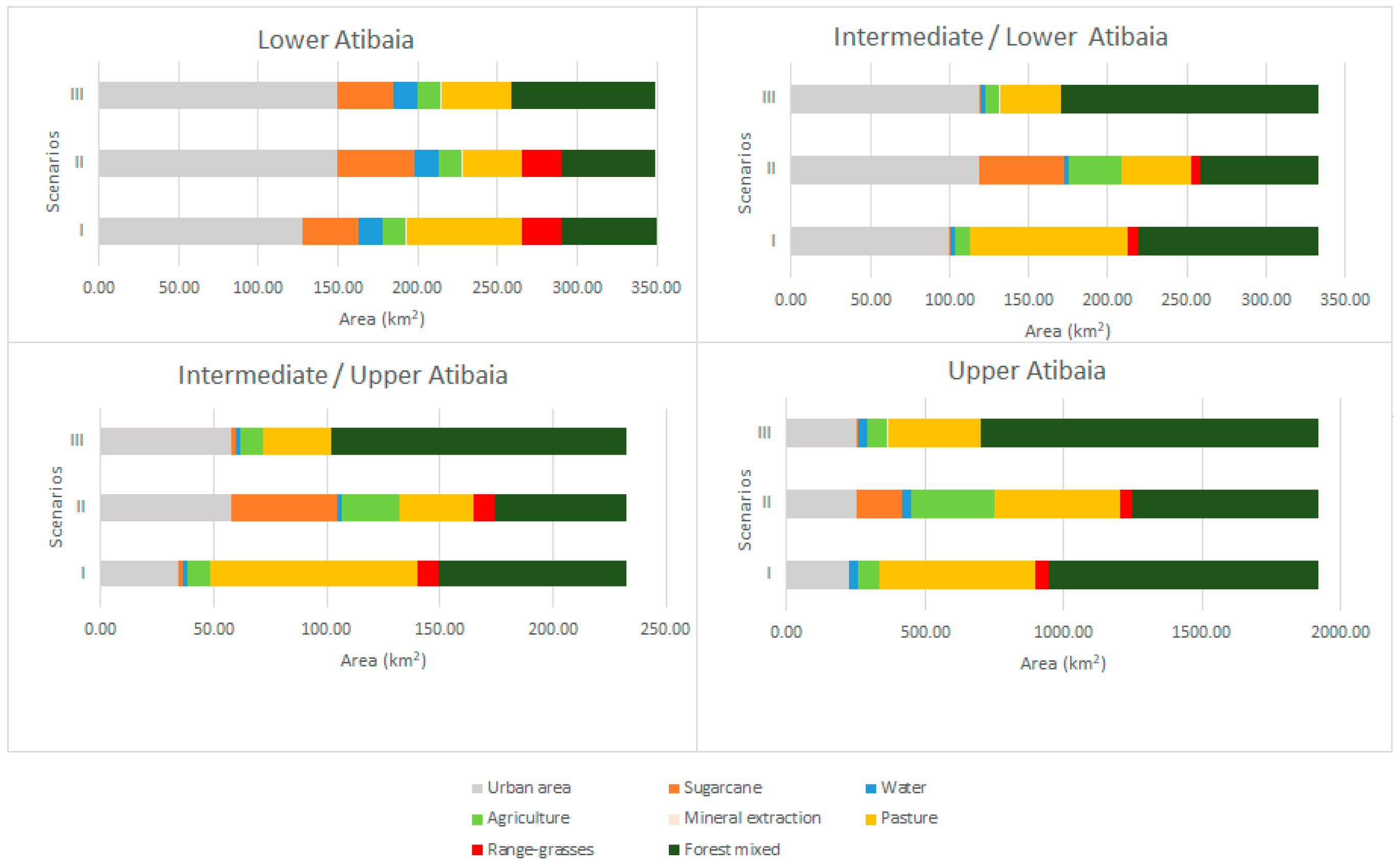
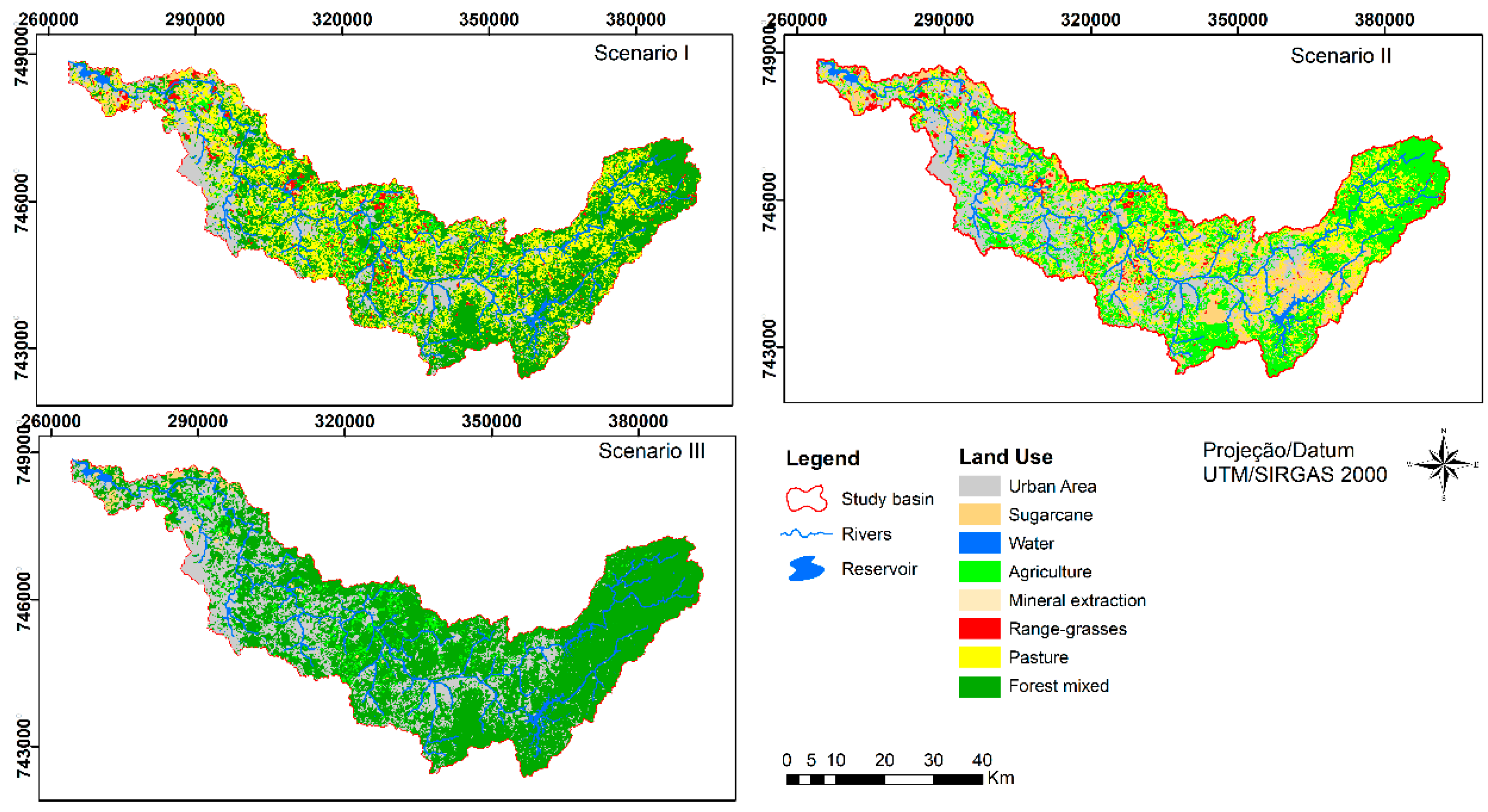
3.2. Description of Land Use Scenarios

The studied land use scenarios were defined based on a comprehensive study done by the [64] that describes the current land use in the studied area and projects possible future land use changes. Scenario I represents the current situation with a predominance of forest and pasture in the rural areas of the Atibaia river basin. Based on this scenario, two possible future scenarios were studied.

Scenario II represents a possible land use evolution if the current trends persist, in which the urban and agriculture areas increase and forest areas recede [5,64,65,66]. The urban area increases by 20%, while 50% of the native forest is replaced by agricultural areas and many crops are substituted by sugar cane.

Scenario III represents a desirable and more beneficial projection of future land use, while still accepting the same urban growth of the trend scenario. To achieve this goal, pasture and all range-grasses areas are substituted by forest areas.

Figure 2 and

Table 2. Land use areas related to each scenario and sub-basin.

Land Uses	Lower Atibaia (km2)			Intermediate Lower Atibaia (km2)			Intermediate/Upper Atibaia (km2)			Upper Atibaia (km2)
	Scen. I	Scen. II	Scen. III	Scen. I	Scen. II	Scen. III	Scen. I	Scen. II	Scen. III	Scen. I	Scen. II	Scen. III
Urban area	127.3	149.0	149.0	99.54	118.46	118.36	34	57.7	57.7	222.1	254.6	254.6
Sugarcane	35.3	48.6	35.2	1.33	53.67	1.33	2.0	47.0	2.0	1.9	160.0	1.9
Mineral Extraction	0.6	0.6	0.6	0.25	0.25	0.25	0	0	0	0.2	0.2	0.2
Water	15.4	15.4	15.4	3.01	3.01	3.01	1.9	1.9	1.9	33.9	33.9	33.9
Agriculture	14.3	14.3	14.3	8.88	33.33	8.82	10.2	25.6	10.1	73.6	299.5	73.5
Pasture	72.3	37.4	43.6	100.03	43.64	38.27	91.8	32.8	30.4	566.3	455.2	336.9
Range-grasses	24.9	24.8	0	6.05	6.05	0	8.8	8.8	0	46.4	46.2	0
Forest mixed	59.2	59.2	91.4	113.80	74.48	162.85	83.4	58.6	130.4	978.6	672.4	1221.0

describe the land use distribution of each scenario in the main sub-basins of the Atibaia river basin. Figure 3 presents the land use maps used as inputs of the SWAT model.

Table 3. Calibrated curve number (CN), maximum canopy storage for each land use (CANMX) and cover and management factor (USLE_C) average values related for each sub-basin.

	Lower Atibaia-4009			Intermediate/Lower Atibaia-3003			Intermediate/Upper Atibaia-3007			Upper Atibaia-3006
Parameters	Scen. I	Scen. II	Scen. III	Scen. I	Scen. II	Scen. III	Scen. I	Scen. II	Scen. III	Scen. I	Scen. II	Scen. III
CN.mgt	50.64	52.82	49.22	50.13	53.19	48.46	40.70	45.27	37.68	36.13	43.87	33.36
CANMX.hru	36.90	26.80	71.00	42.60	27.10	69.00	43.20	28.20	70.00	45.90	29.47	70.00
USLE_C.crop	0.001	0.1	0.0005	0.005	0.2	0.0004	0.005	0.14	0.0004	0.005	0.17	0.0004

presents the average CN, CANMX and USLE_C for each sub-basin and each scenario. The current conditions at the Lower Atibaia sub-basin are represented by an USLE_C of 0.001, indicating the absence of conservation practices in the watershed, mainly due to pasture and sugar cane areas without proper management. The conditions at the other sub-basins with smaller areas of sugar cane are better with an USLE_C within the range of 0.004–0.005. Future scenarios II and III assume an improvement of management practices.

4. Results and Discussion

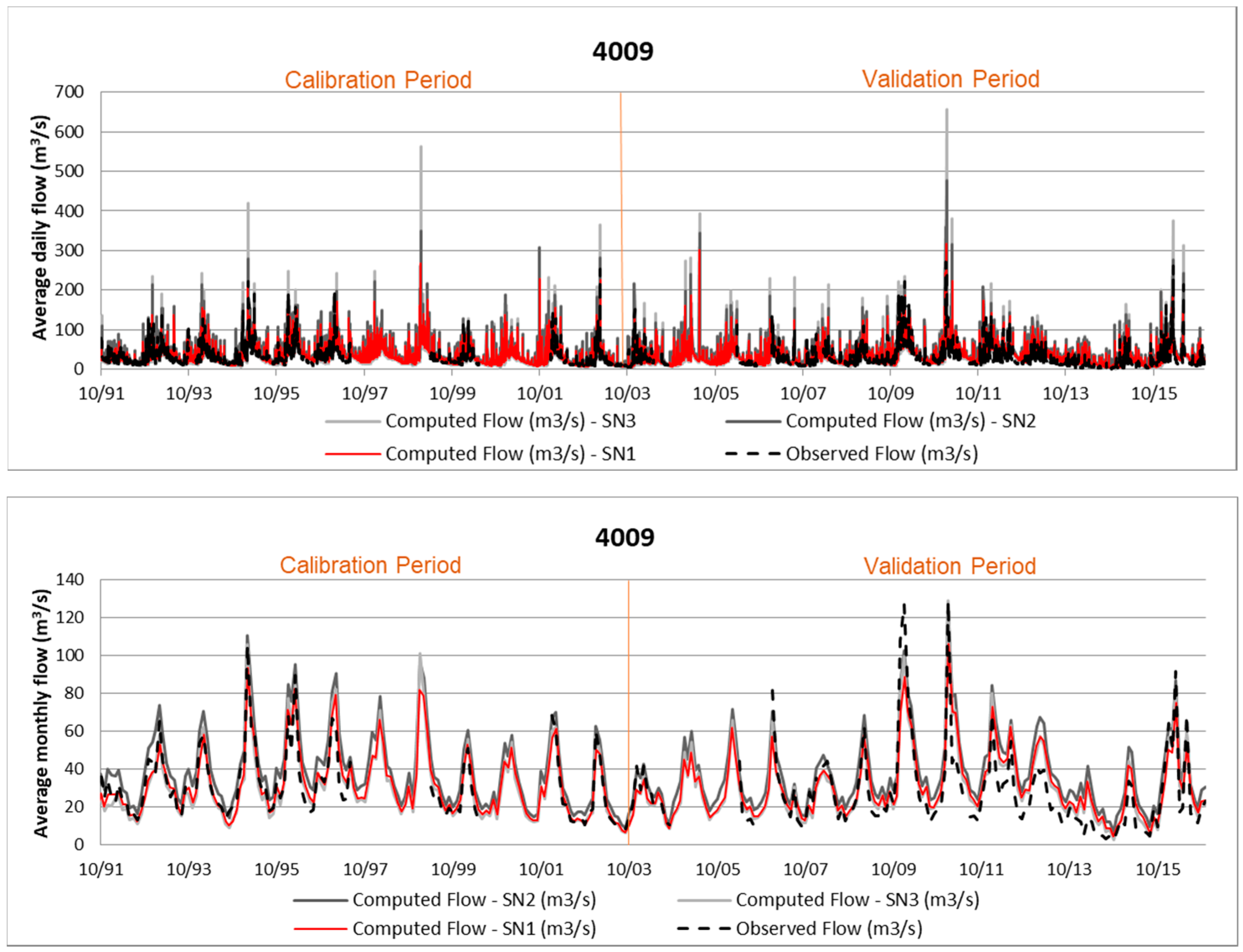
4.1. SWAT Performance

The sensitivity analysis indicated the 10 parameters that stream flow is most sensitive to, as measured by p-value and t-stat values (

Table 4. Sensitivity analysis of SWAT model parameters before the calibration and validation process and for the final results.

Parameters	Before SWAT Simulation
	t-Stat	p-Value
CN.mgt	−1.82	0.31
SOL.awc	−1.50	0.37
CANMX.hru	1.25	0.43
GW_REVAP.gw	−1.13	0.46
ESCO.hru	1.11	0.47
SURLAG.hru	−0.74	0.59
ALPHA_BF.gw	−0.71	0.60
SLSOIL.hru	0.51	0.70
CNCOEF.bsn	0.45	0.73
RCHRG_DP.gw	0.41	0.75

). The t-stat is used to identify the relative significance of each parameter, with a larger absolute value meaning greater sensitivity. The p-value determines the significance of the sensitivity, and values close to zero indicate the most significant parameters [67]. Among these 10 parameters, CN and CANMX are the two land-use related parameters that significantly affect stream flow. The cover and management factor (USLE_C) from the MUSLE equation does not affect streamflow but is the most important parameter regarding the sediment yield.

Table 5. Calibrated parameters of SWAT model with their default and calibrated values.

	Parameters	Definition	Unit	Range	Default Value	Calibrated Value
Water	GW_REVAP.gw	Groundwater “revap” coefficient	-	0.02 to 0.2	0.02	0.04
	ALPHA_BF.gw	Base flow alpha factor	days	0 to 1	0.048	0.001
	RCHRG_DP.gw	Deep aquifer percolation fraction	mm	0 to 1	0.05	0.12
	CANMX.hru (Maximum canopy storage)	Urban area	mm	0 to 100	0	15
		Sugarcane				40
		Water				0
		Agriculture				40
		Mineral extraction				0
		Pasture				20
		Range-grasses				20
		Forest mixed				80
	ESCO.hru	Soil evaporation compensation factor	-	0.01 to 1	0.95	0.6
	SLSOIL.hru	Slope length for lateral subsurface flow	m	0 to 150	0	40
	SURLAG.hru	Surface runoff lag coefficient	-	0 to 1	2	1
	CNCOEF.bsn	Weighting coefficient for calculating retention dependent of plant evapotranspiration	-	0.5 to 2	2	1.5
	CN.mgt	Initial curve number for moisture condition II	-	0 to 100	Varies	0.7 a
	SOL.awc	Available water capacity of soil layer	mm/mm	0 to 1	Varies	0.7 a
	USLE_C.crop (The cover and management factor)	Sugarcane	-	0 to 1	0.001	0.050 3
		Water			0	0 2
		Agriculture			0.2	0.200 1
		Pasture			0.003	0.0075 3,4
		Range-grasses			0.003	1 3
		Forest mixed			0.001	0.0004 1
Sediment	USLE_P.mgt	USLE support practice factor	-	0 to 1	1	0.8
	CH_COV1.rte	Channel erodibility factor	-	−0.05 to 0.6	0	0.1
	CH_COV2.rte	Channel cover factor	-	−0.001 to 1	0	0.1
	LAT_SED.hru	Sediment concentration in lateral flow and groundwater flow	mg/L	0 to 5000	0	3000

^a Multiplying factor to be applied to the parameter original value. Values adapted by ¹ [46] ² [47] ³ [45] ⁴ [36].

presents the set of parameter values that leads to a satisfactory model performance. For each parameter, the table shows its default value and the value obtained after calibration.

The initial curve number values for moisture condition II (CN) were reduced by 30% homogeneously across the basin to support base flow and infiltration, and available water capacity of the topsoil layer (SOL_AWC) was reduced by 30% uniformly across the basin to decrease the soil holding capacity, to delay the flow reaching the river and to increase the base flows. The soil evaporation compensation factor (ESCO) was reduced to 0.6 to promote evaporation from the deepest soil layers.

The groundwater “revap” coefficient (GW_REVAP) controls the water flow from the shallow aquifer to the unsaturated zone. This parameter was set to 0.04, which means more water available for the base flow. The deep aquifer percolation fraction (RCHRG_DP) was set to 0.12, which indicates that 12% of soil percolation water is directed to a deep aquifer.

The maximum canopy storage (CANMX) was defined between 0 and 80 to describe different canopy storage capacity to intercept the precipitation for each crop. The base flow alpha factor (ALPHA_BF) is used by the model to calculate the base flow and was adjusted to 0.001.

The slope length for lateral subsurface flow (SLSOIL), associated with the interflow source, was set at 40 m and the surface runoff lag coefficient (SURLAG), related to the daily surface runoff amount that discharges into the main channel, was set 1. Weighting coefficient for calculating retention dependent of plant evapotranspiration (CNCOEF) was adjusted to 1.6

To reproduce sediment yield, the cover and management factor (USLE_C) was defined between 0 and 1 for different land uses. The USLE equation support practice parameter (USLE_P) was set to 0.8, recognizing the presence of conservation practices in the watershed.

The channel erodibility factor (CH_COV1) and the channel coverage factor (CH_COV2) were adjusted to 0.1 representing a low vulnerability to channel erosion. The sediment concentration in lateral flow and groundwater flow (LAT_SED) was set at 3000 to represent the sediment yield in lateral and groundwater flow.

The model calibration and validation process is influenced by the choice of the objective function and affected by the equifinality problem [68]. To alleviate these issues, a manual approach was adopted which considered the model’s ability to reproduce streamflow and sediment yield at several monitoring stations. By carefully selecting the parameter values and considering multiple sites, two objectives and the equifinality problem are mitigated. A complete description of the calibration process and the parameters selected is presented in [20,21].

Figure 4 compares the simulated and observed streamflow at the most downstream gage, obtained during calibration and validation. The model can adequately simulate the overall variation of stream, as well as both its minimum and the maximum values, although some extreme high daily values are overestimated. The Nash-Sutcliffe coefficient is usually higher than 0.5 when computed from daily values and higher than 0.7 when computed from monthly values (

Table 6. Statistic evaluation of simulated versus observed average daily and monthly streamflow data.

Gages	Daily						Monthly
	Calibration			Validation			Calibration			Validation
	NSE	Pbias	r2	NSE	Pbias	r2	NSE	Pbias	r2	NSE	Pbias	r2
3006	0.54	1.87	0.38	0.28	−24.54	0.41	0.83	1.03	0.64	0.60	−8.92	0.62
3007	0.48	−10.00	0.43	0.36	−14.04	0.47	0.79	7.71	0.83	0.70	−4.93	0.71
3003	0.69	−3.46	0.48	0.49	−19.34	0.52	0.85	−8.50	0.71	0.69	−5.46	0.72
4009	0.75	−21.21	0.60	0.60	−16.65	0.54	0.96	−4.94	0.90	0.81	−15.84	0.80

). The model results are slightly worse for the upstream sub-basin.

Figure 5 compares observed sediment yield values with the model simulated results, showing that SWAT can replicate the scale and the variation pattern of the sediment yield, although not with precision.

Table 7. Statistic evaluation of simulated versus observed sediment yield, total nitrogen and phosphorus load.

Gage	Sediment Yield
	NSE	Pbias	r2
2605	0.06	39.50	0.30

presents the computed performance indicators for sediment yield. The low monitoring frequency of sediment transport (bimonthly) and the fact that most data has been collected during low flows hinders a detailed evaluation of the model performance.

Based on these streamflow and sediment yield results, for both the calibration and validations periods, we concluded that the model is adequate for estimating the impacts of different land use scenarios.

4.2. Scenario Simulation

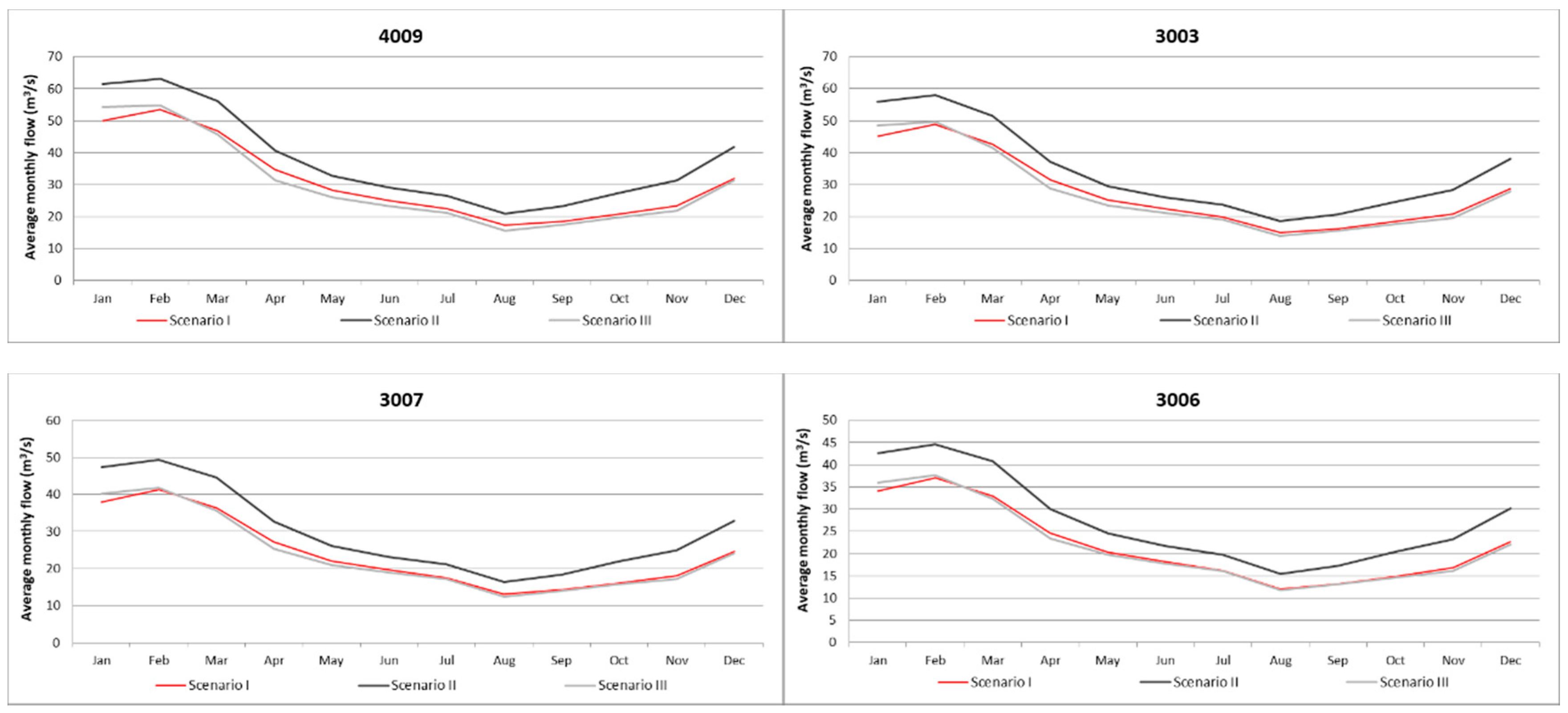
4.2.1. Streamflow

The conversion of forests to agriculture, sugarcane and urban uses (scenario II) leads to an increase of streamflow, as evapotranspiration decreases and surface flow, percolation and groundwater flow increases (

Table 8. Annual mean water balance variables of four Atibaia sub-basins according to SWAT, from 1990 to 2016 (in mm).

Variable	4009			3003			3007			3006
	Scen. I	Scen. II	Scen. III	Scen. I	Scen. II	Scen. III	Scen. I	Scen. II	Scen. III	Scen. I	Scen. II	Scen. III
P	1594	1594	1594	1594	1594	1594	1404	1404	1404	1404	1404	1404
PET	1939	1939	1939	1939	1939	1939	1924	1924	1924	1924	1924	1924
ET	1032	966	1078	1009	953	1044	1021	951	1072	1076	1049	1112
Revap	77	77	77	77	77	77	58	58	58	54	54	54
Perc	474	527	381	449	469	342	221	235	151	116	121	99
SurQ	45	56	100	66	100	153	3	58	72	29	54	63
GwQ	348	396	260	327	345	225	137	150	76	49	57	39
LatQ	42	45	34	69	70	54	161	162	111	186	182	134
Deep	57	63	46	54	56	41	26	28	18	14	15	12
Flow_out	444	517	412	482	538	447	314	378	271	283	300	243

Where: P: Precipitation (mm); PET: Potential evapotranspiration (mm); ET: Real evapotranspiration (mm); Perc: Percolation (mm); SurQ: Surface runoff contribution to streamflow (mm); GwQ: Groundwater contribution to streamflow (mm/day); LatQ: Lateral flow contribution to streamflow (mm); Deep: Deep Percolation; Flow_out: Average daily streamflow out of reach during time step (mm).

). Conversely the replacement of pasture, range-grasses and agriculture by forest (scenario III) leads to an increase in evaporation and surface flow and to a decrease of streamflow, lateral flow, percolation and groundwater flow. This result is in line with findings that show that forest development promotes infiltrations and reduces surface streamflow [14,69,70,71,72,73,74,75].

The differences between the scenarios can be attributed to the distinct evapotranspiration rates of each crop arising from their different root systems, as well as to changes in the ratio of surface runoff versus infiltration which is dependent on land use and soil cover [11].

While land-cover change may have a moderate impact on average annual flow, it can significantly influence seasonal and monthly streamflow. Figure 6 presents the average monthly streamflow estimated at the four hydrometric stations for each land use scenario. The precipitation seasonal variability of precipitation leads to high flows from December to April and to low flows from July to October.

In general, scenario II shows an increase in the streamflow which is higher during wet months. The increase of agricultural and urban areas and the decrease of soil cover associated with this scenario (Table 4) results in higher average CN values and lower CANMX values. This trend is mainly associated with substitution of forest areas by agriculture. In turn, these changes lead to a faster water movement throughout the river basin, a lower retention time, a decrease of evapotranspiration and to an increase of surface and lateral flow (

Table 9. Comparison of annual average sediment yield sediment yield values (1990 to 2016).

Gage	Annual Average Sediment Yield (ton/year)
	Scenario I	Scenario II	Scenario III
2605	73941	97078 (+24%)	75806 (+2%)

). This change of the runoff–precipitation ratio is more striking in the rainy periods and less in the dry periods.

The significant reduction in evapotranspiration in the upper sub-basin is mainly due to the replacement of forests by agriculture. The forest areas (Forest mixed—FRST) have a Leaf Area Index (LAI) value of 5 mm and the canopy height ($h_{c,mx}$) of 6 cm, while the agricultural areas (Agriculture Land Generic—AGRL) have a LAI of 3 mm and hc of 1 cm. The reduction in the value of these parameters influences the canopy storage and contributes to the decrease in the precipitation interceptions and evaporation in all sub-basins.

In scenario III, the increase of forest areas over the pasture and range grasses areas, results in lower CN values and higher CANMX values, mainly due to increases in the LAI and $h_{c,mx}$ values, respectively from 4 mm and 0.5 cm for pasture and 2.5 mm and 1 cm for range grasses to 5 mm and 6 cm for forests.

However, the simultaneous trend towards larger urban areas counterbalances the increase of evapotranspiration and decrease of lateral flow and streamflow due to forestation, and scenario III becomes very similar to scenario I. The small increase of streamflow in January and the small decrease in the dry season small change is due to the increase in temperature during the wet periods that has significant impact on the growing stage of the vegetation in function of the evapotranspiration, and consequently in this period the base flow becomes important to contribute to the streamflow.

These results are in line with the studies performed by [3,13,76].

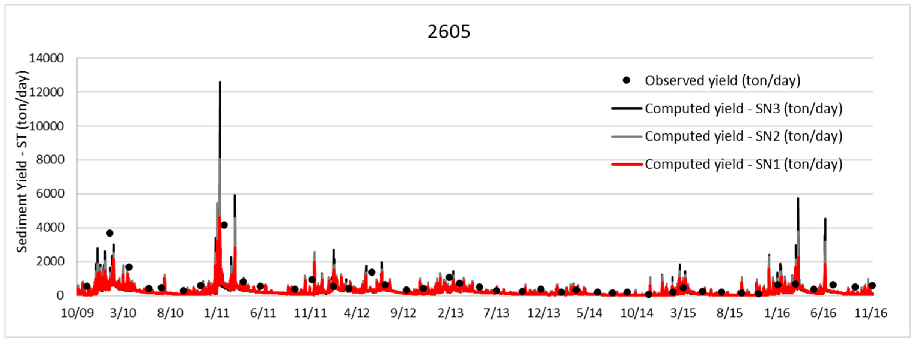
4.2.2. Sediment Yield

Table 9 compares the annual average sediment yield estimated from each scenario for the 1990–2016 period.

The replacement of forest areas by perennial agriculture (scenario II) leads to an increase in annual average sediment yield values (+24%) because the original forest areas ensure a superior soil cover over a longer period of the year. Even when perennial agricultures are grown with good conservation practice, these areas produce high amounts of sediment due to their relatively low soil cover, as compared to forest areas. This result was also obtained by [77,78].

Scenario III shows a slight increase in annual average sediment yield values (+2%). Despite the increase of forest areas that ensures soil cover, the significant urban growth contributes to the increase in surface flow and, consequently, to a larger amount of sediment that is transported into rivers. According to [79], the increased runoff in urban areas is very effective at eroding the available sediment sources.

Figure 7 plots the average monthly sediment yield for each scenario. The sediment yield behavior is very similar to the streamflow because the SWAT model uses to the MUSLE equation, which computes the sediment yield from runoff volume and peak flow rate [80]. While the USLE and RUSLE models estimate average annual gross erosion as a function of rainfall energy, MUSLE uses a runoff factor that is recalculated every day, which is appropriate for the simulation of erosion and sediment yield within each HRU at a daily time step [7,80,81,82]. Sediment yield prediction also is improved because runoff is a function of antecedent moisture condition as well as rainfall energy [38,83]. The need for delivery ratios required by USLE is eliminated because the runoff factor represents energy used in detaching and transporting sediment [7].

Ref. [81] show a comparison of the erosion prediction models from USLE, MUSLE and RUSLE in a Mediterranean watershed, in the case of Wadi Gazouana (NW of Algeria).

5. Conclusions

The effects of land use change on the streamflow and sediment yield of the Atibaia river basin were estimated using SWAT. The model parameters that have the largest impacts on streamflow and sediment yield are the initial curve number for moisture condition II (CN), the maximum canopy storage for each land use (CANMX) and the cover and management factor (USLE_C). Other parameters also related to land use are the maximum leaf area index (LAI_mx), the canopy height ($h_{c,mx}$), the total heat units required for plant maturity ($PHU$), and the amount of residue on the soil surface ($rs{d}_{surf}$). The model was setup to automatically update these parameters from each land use map.

Two different land use change scenarios were applied to the study basin and the streamflow and sediment yield outputs were compared with the current situation. The expansion of perennial agriculture and urban areas at the expense of forest areas leads to an increase of streamflow, as percolation and groundwater flow increases and evapotranspiration decreases. The increase of surface runoff and streamflow leads to an increase of sediment yield. The expansion of forest areas over pasture, range-grasses and agriculture leads to a decrease in streamflow and to a slight increase in sediment yield as evaporation and surface flow increase and the lateral flow, the deep percolation, the groundwater flow and the percolation decreases. Both land use scenarios maintained the seasonal variation of streamflow and sediment yield, following the precipitation pattern in the wet and dry periods.

The identification and appropriate parameters change in the SWAT model can provide real estimates of the magnitudes in the land use changes, which were verified in this study. Such information can be used as an instrument for proposing improvements in the basin environmental quality and management.

It should also be noted that land use changes often lead to other significant alterations of the river basin, namely in the drainage network. A trend towards urbanization brings along changes in the river channels alignments, profiles, cross-sections, bed and bank materials and conveyance capacity. In general, the artificialization of the river network speeds the water velocity through the river network, leading to higher peak flows. A trend towards a renaturalization of the river basin may lead to changes in the opposite direction. The impacts of these alterations may be significant, and although they can also be simulated in SWAT by modifying the flow routing parameters, this was not performed in the current study.

References

1. Kuhnle, R.A.; Bingner, R.L.; Foster, G.R.; Grissinger, E.H. Effect of land use changes on sediment transport in Goodwin Creek. Water Resour. Res. 1996, 32, 3189–3196. [Google Scholar] [CrossRef]
2. Memarian, H.; Balasundram, S.K.; Abbaspour, K.C.; Talib, J.B.; Boon Sung, C.T.; Sood, A.M. SWAT-based hydrological modelling of tropical land-use scenarios. Hydrol. Sci. J. 2014, 59, 1808–1829. [Google Scholar] [CrossRef]
3. Pikounis, M.; Varanou, E.; Baltas, E.; Dassaklis, A.; Mimikou, M. Application of the SWAT model in the Pinios River basin under different land-use scenarios. Glob. Nest Int. J. 2003, 5, 71–79. [Google Scholar]
4. Quilbé, R.; Rousseau, A.N.; Moquet, J.S.; Savary, S.; Ricard, S.; Garbouj, M.S. Hydrological responses of a watershed to historical land use evolution and future land use scenarios under climate change conditions. Hydrol. Earth Syst. Sci. Discuss. 2008, 12, 101–110. [Google Scholar]
5. Rodrigues, E.L.; Elmiro, M.A.; Braga, F.D.A.; Jacobi, C.M.; Rossi, R.D. Impact of changes in land use in the flow of the Pará River Basin, MG. Rev. Bras. Eng. Agrícola E Ambient. 2015, 19, 70–76. [Google Scholar] [CrossRef] [Green Version]
6. Arnold, J.G.; Fohrer, N. SWAT2000: Current capabilities and research opportunities in applied watershed modelling. Hydrol. Process. Int. J. 2005, 19, 563–572. [Google Scholar] [CrossRef]
7. Neitsch, S.L.; Arnold, J.G.; Kiniry, J.R.; Williams, J.R. Soil and Water Assessment Tool Theoretical Documentation Version 2009, 2011; Texas Water Resources Institute: College Station, TX, USA, 2009. [Google Scholar]
8. U.S. Army Corps of Engineers Hydrologic Engineering Center (USACEHEC-1998). HEC-HMS Hydrologic Modeling System User’s Manual; USACE-HEC: Davis, CA, USA, 1998. [Google Scholar]
9. Artan, G.A.; Asante, K.; Smith, J.; Pervez, S.; Entenmann, D.; Verdin, J.P.; Rowland, J. Users Manual for the Geospatial Stream Flow Model (GeoSFM); Geological Survey: Reston, VA, USA, 2008. [Google Scholar]
10. Aparna, P.; Raunak, M.; Patra, K.C. Impact of Landuse Land Cover Change on Streamflow of Upper Baitarani River Basin using SWAT. MTech Thesis, 2018. Available online: http://dspace.nitrkl.ac.in/dspace/bitstream/2080/2948/1/2018_STIWM_ADas_Impact.pdf (accessed on 15 June 2020).
11. Baker, T.J.; Miller, S.N. Using the Soil and Water Assessment Tool (SWAT) to assess land use impact on water resources in an East African watershed. J. Hydrol. 2013, 486, 100–111. [Google Scholar] [CrossRef]
12. Ghaffari, G.; Keesstra, S.; Ghodousi, J.; Ahmadi, H. SWAT-simulated hydrological impact of land-use change in the Zanjanrood basin, Northwest Iran. Hydrol. Process. Int. J. 2010, 24, 892–903. [Google Scholar] [CrossRef]
13. Marhaento, H.; Booij, M.J.; Rientjes, T.H.M.; Hoekstra, A.Y. Attribution of changes in the water balance of a tropical catchment to land use change using the SWAT model. Hydrol. Process. 2017, 31, 2029–2040. [Google Scholar] [CrossRef]
14. Woldesenbet, T.A.; Elagib, N.A.; Ribbe, L.; Heinrich, J. Hydrological responses to land use/cover changes in the source region of the Upper Blue Nile Basin, Ethiopia. Sci. Total Environ. 2017, 575, 724–741. [Google Scholar] [CrossRef]
15. Alkimim, A.; Sparovek, G.; Clarke, K.C. Converting Brazil’s pastures to cropland: An alternative way to meet sugarcane demand and to spare forestlands. Appl. Geogr. 2015, 62, 75–84. [Google Scholar] [CrossRef]
16. Strassburg, B.B.; Brooks, T.; Feltran-Barbieri, R.; Iribarrem, A.; Crouzeilles, R.; Loyola, R.; Soares-Filho, B. Moment of truth for the Cerrado hotspot. Nat. Ecol. Evol. 2017, 1, 1–3. [Google Scholar] [CrossRef] [PubMed]
17. Lapola, D.M.; Martinelli, L.A.; Peres, C.A.; Ometto, J.P.; Ferreira, M.E.; Nobre, C.A.; Joly, C.A. Pervasive transition of the Brazilian land-use system. Nat. Clim. Chang. 2014, 4, 27–35. [Google Scholar] [CrossRef] [Green Version]
18. Soares-Filho, B.; Rajão, R.; Macedo, M.; Carneiro, A.; Costa, W.; Coe, M.; Alencar, A. Cracking Brazil’s forest code. Science 2014, 344, 363–364. [Google Scholar] [CrossRef]
19. Arnold, J.G.; Moriasi, D.N.; Gassman, P.W.; Abbaspour, K.C.; White, M.J. SWAT: Model use, calibration, and validation. Trans. ASABE 2012, 55, 1491–1508. [Google Scholar] [CrossRef]
20. Santos, F.M.; Oliveira, R.P.; Mauad, F.F. Evaluating a parsimonious watershed model to estimate streamflow, soil loss and river contamination using two case studies in Tietê river basin, São Paulo, Brazil. J. Hydrol. Reg. Stud. 2020, 29, 100–685. [Google Scholar]
21. Santos, F.M.; Oliveira, R.P.; Mauad, F.F. Lumped versus Distributed Hydrological Modeling of the Jacaré-Guaçu Basin, Brazil. J. Environ. Eng. 2018, 144, 04018056. [Google Scholar] [CrossRef]
22. Sharpley, A.N.; Williams, J.R. EPIC Erosion/Productivity Impact Calculator: 1. Model Documentation; USA Department of Agriculture Technical Bulletin No. 1768; USA Government Printing Office: Washington, DC, USA, 1990.
23. Hawkins, A.J.S.; Bayne, B.L. Seasonal variation in the relative utilization of carbon and nitrogen by the mussel Mytilus edulis: Budgets, conversion efficiencies and maintenance requirements. Marine ecology progress series. Oldendorf 1985, 25, 181–188. [Google Scholar] [CrossRef]
24. Haan, C.T.; Barfield, B.J.; Hayes, J.C. Design Hydrology and Sedimentology for Small Catchments; Elsevier: Amsterdam, The Netherlands, 1994. [Google Scholar]
25. Wang, Q.; Liu, R.; Men, C.; Guo, L.; Miao, Y. Effects of dynamic land use inputs on improvement of SWAT model performance and uncertainty analysis of outputs. J. Hydrol. 2018, 563, 874–886. [Google Scholar] [CrossRef]
26. Alibuyog, N.R.; Ella, V.B.; Reyes, M.R.; Srinivasan, R.; Heatwole, C.; Dillaha, T. Predicting the effects of land use change on runoff and sediment yield in Manupali River sub watersheds using the SWAT model. Int. Agric. Eng. J. 2009, 18, 15. [Google Scholar]
27. Can, T.; Xiaoling, C.; Jianzhong, L.; Gassman, P.W.; Sabine, S.; José-Miguel, S.P. Assessing impacts of different land use scenarios on water budget of Fuhe River, China using SWAT model. Int. J. Agric. Biol. Eng. 2015, 8, 95–109. [Google Scholar]
28. Neitsch, S.L.; Arnold, J.G.; Kiniry, J.R.; Williams, J.R.; King, K.W. Soil and Water Assessment Tool Theoretical Documentation, Version 2000 (Draft); Blackland Research Center, Texas Agricultural Experiment Station: Temple, TX, USA, 2001. [Google Scholar]
29. Yen, H.; White, M.J.; Jeong, J.; Arabi, M.; Arnold, J.G. Evaluation of alternative surface runoff accounting procedures using SWAT model. Int. J. Agric. Biol. Eng. 2015, 8, 64–68. [Google Scholar]
30. Mulungu, D.M.; Munishi, S.E. Simiyu River catchment parameterization using SWAT model. Phys. Chem. EarthParts A/B/C 2007, 32, 1032–1039. [Google Scholar] [CrossRef]
31. Tarigan, S.; Wiegand, K.; Slamet, B. Minimum forest cover required for sustainable water flow regulation of a watershed: A case study in Jambi Province, Indonesia. Hydrol. Earth Syst. Sci. 2018, 22, 581–594. [Google Scholar] [CrossRef] [Green Version]
32. Sinnathamby, S.; Douglas-Mankin, K.R.; Craige, C. Field-scale calibration of crop-yield parameters in the Soil and Water Assessment Tool (SWAT). Agric. Water Manag. 2017, 180, 61–69. [Google Scholar] [CrossRef] [Green Version]
33. Hall, R.J.; Davidson, D.P.; Derek, R.P. Ground and remote estimation of leaf area index in Rocky Mountain forest stands, Kananaskis, Alberta. Can. J. Remote Sens. 2003, 29, 411–427. [Google Scholar] [CrossRef]
34. Schaffrath, D.; Barthold, F.K.; Bernhofer, C. Spatiotemporal variability of grassland vegetation cover in a catchment in Inner Mongolia, China, derived from MODIS data products. Plant Soil 2010, 340, 181–198. [Google Scholar] [CrossRef]
35. White, J.D.; Running, S.W.; Nemani, R.; Keane, R.E.; Ryan, K.C. Measurement and remote sensing of LAI in Rocky Mountain montane ecosystems. Can. J. For. Res. 1997, 27, 1714–1727. [Google Scholar] [CrossRef]
36. Wei, Z.; Zhang, B.; Liu, Y.; Xu, D. The application of a modified version of the SWAT model at the daily temporal scale and the hydrological response unit spatial scale: A case study covering an irrigation district in the Hei River Basin. Water 2018, 10, 1064. [Google Scholar] [CrossRef] [Green Version]
37. Guse, B.; Reusser, D.E.; Fohrer, N. How to improve the representation of hydrological processes in SWAT for a lowland catchment–temporal analysis of parameter sensitivity and model performance. Hydrol. Process. 2014, 28, 2651–2670. [Google Scholar] [CrossRef]
38. Nossent, J.; Elsen, P.; Bauwens, W. Sobol’sensitivity analysis of a complex environmental model. Environ. Model. Softw. 2011, 26, 1515–1525. [Google Scholar] [CrossRef]
39. Williams, J.R.; Berndt, H.D. Sediment yield prediction based on watershed hydrology. Trans. ASAE 1977, 20, 1100–1104. [Google Scholar] [CrossRef]
40. Arabi, M.; Frankenberger, J.R.; Engel, B.A.; Arnold, J.G. Representation of agricultural conservation practices with SWAT. Hydrol. Process. Int. J. 2008, 22, 3042–3055. [Google Scholar] [CrossRef]
41. Betrie, G.D.; Mohamed, Y.A.; Van Griensven, A.; Srinivasan, R. Sediment management modelling in the Blue Nile Basin using SWAT model. 1foldr Import 2019-10-08 Batch 5. Hydrol. Earth Syst. Sci. 2011, 15, 807–818. [Google Scholar] [CrossRef] [Green Version]
42. Jeon, D.J.; Ki, S.J.; Cha, Y.; Park, Y.; Kim, J.H. New methodology of evaluation of best management practices performances for an agricultural watershed according to the climate change scenarios: A hybrid use of deterministic and decision support models. Ecol. Eng. 2018, 119, 73–83. [Google Scholar] [CrossRef]
43. Wischmeier, W.H.; Smith, D.D. Predicting Rainfall Erosion Losses: A Guide to Conservation Planning; Department of Agriculture, Science and Education Administration: Washington, DC, USA, 1978. [Google Scholar]
44. Lee, M.; Park, G.; Park, M.; Park, J.; Lee, J.; Kim, S. Evaluation of non-point source pollution reduction by applying Best Management Practices using a SWAT model and QuickBird high resolution satellite imagery. J. Environ. Sci. 2010, 22, 826–833. [Google Scholar] [CrossRef]
45. Bertoni, J.; Lombardi Neto, F. Conservação do Solo; Ícone: São Paulo, Brazil, 2010. [Google Scholar]
46. Cavalieri, A. Estimativa da Adequação de Uso das Terras da Quadrícula de Moji Mirim (SP), Utilizando Diferentes Métodos; Tese de Doutorado, Faculdade de Engenharia Agrícola-UNICAMP: Campinas, Brazil, 1998. [Google Scholar]
47. Farinasso, M.; Carvalho Júnior, O.A.D.; Guimarães, R.F.; Gomes, R.A.T.; Ramos, V.M. Avaliação qualitativa do potencial de erosão laminar em grandes áreas por meio da EUPS utilizando novas metodologias em SIG para os cálculos dos seus fatores na região do Alto Parnaíba-PI/MA. Rev. Bras. De Geomorfol. 2006, 7, 73–85. [Google Scholar] [CrossRef]
48. Bonumá, N.B.; Rossi, C.G.; Arnold, J.G. Hydrology evaluation of the Soil and Water Assessment Tool considering measurement uncertainty for a small watershed in Southern Brazil. Appl. Eng. Agric. 2013, 29, 189–200. [Google Scholar] [CrossRef]
49. Kim, H.; Parajuli, P.B. Impacts of Reservoir Operation in the SWAT Model Calibration. In 2012 Dallas, Texas, July 29–August 1 2012; American Society of Agricultural and Biological Engineers: St. Joseph, MI, USA, 2012; p. 1. [Google Scholar]
50. Lenhart, K.; Eckhardt, N.; Fohrer, F.H.G. Comparison of two different approaches of sensitivity analysis. Phys. Chem. Earth 2002, 27, 645–654. [Google Scholar] [CrossRef]
51. Malagó, A.; Bouraoui, F.; Vigiak, O.; Grizzetti, B.; Pastori, M. Modelling water and nutrient fluxes in the Danube River Basin with SWAT. Sci. Total Environ. 2017, 603, 196–218. [Google Scholar] [CrossRef]
52. Me, W.; Abell, J.M.; Hamilton, D.P. Effects of hydrologic conditions on SWAT model performance and parameter sensitivity for a small, mixed land use catchment in New Zealand. Hydrol. Earth Syst. Sci. 2015, 19, 4127–4147. [Google Scholar] [CrossRef] [Green Version]
53. Strauch, M.; Lima, J.E.; Volk, M.; Lorz, C.; Makeschin, F. The impact of Best Management Practices on simulated streamflow and sediment load in a Central Brazilian catchment. J. Environ. Manag. 2013, 127, S24–S36. [Google Scholar] [CrossRef] [PubMed]
54. Tolson, B.A.; Shoemaker, C.A. Cannonsville reservoir watershed SWAT2000 model development, calibration and validation. J. Hydrol. 2007, 337, 68–86. [Google Scholar] [CrossRef]
55. Nash, J.E.; Sutcliffe, J.V. River flow forecasting through conceptual models part I—A discussion of principles. J. Hydrol. 1970, 10, 282–290. [Google Scholar] [CrossRef]
56. Krause, P.; Boyle, D.P.; Bãse, F. Comparison of different efficiency criteria for hydrological model assessment. Adv. Geosci. 2005, 5, 89–97. [Google Scholar] [CrossRef] [Green Version]
57. Sigrh–Sistema Integrado De Gerenciamento De Recursos Hídricos. Situação de Recursos Hídricos do Estado de São Paulo: 2015, 6th ed.; Governo do Estado de São Paulo, Secretaria de Saneamento e Recursos Hídricos, Coordenadoria de Recursos Hídricos: São Paulo, Brazil, 2017.
58. Freire, O.; Gimenez, J.; Pessoti, J.E.; Carraro, E. Solos da Bacia do Broa; Universidade Federal de São Paulo: São Carlos, Brazil, 1978; 125p. [Google Scholar]
59. Lombardi Neto, F.; Bellinazzi, R., Jr.; Galeti, P.A.; Lepsch, I.; Oliveira, J.D. Nova abordagem para cálculo de espaçamento entre terraços. In Simpósio Sobre Terraceamento Agrícola; Lombardi Neto, B., Jr., Ed.; Fundação Cargill: Campinas, Brazil, 1989; pp. 99–124. [Google Scholar]
60. Oliveira, J.B.; Prado, H. Levantamento Pedológico Semidetalhado do Estado de São Paulo: Memorial Descritivo; IAC: Campinas, Brazil, 1984; 110p. [Google Scholar]
61. Saxton, K.E.; Rawls, W.J. Soil water characteristic estimates by texture and organic matter for hydrologic solutions. Soil Sci. Soc. Am. J. 2006, 70, 1569–1578. [Google Scholar] [CrossRef] [Green Version]
62. TECNOGEO. Mapeamento do uso e Cobertura do solo da UGRHI 5 (PCJ)-Escala 1:25.000-Coordenadoria de Planejamento Ambiental, Instituto Geológico; Secretaria do Meio Ambiente do Estado de São Paulo: São Paulo, Brazil, 2013. [Google Scholar]
63. Rudorff, B.F.T.; Aguiar, D.A.; Silva, W.F.; Sugawara, L.M.; Adami, M.; Moreira, M.A. Studies on the rapid expansion of sugarcane for ethanol production in São Paulo State (Brazil) using Landsat data. Remote Sens. 2010, 2, 1057–1076. [Google Scholar] [CrossRef] [Green Version]
64. Comitê das Bacias Hidrográficas dos rios Piracicaba, Capivari e Jundiaí (CBH-PCJ). Plano de Bacias Hidrográfcas dos rios Piracicaba, Capivari e Jundiaí. Relatório Final; CBH-PCJ: São Paulo, Brazil, 2013. [Google Scholar]
65. Demanboro, A.C.; Laurentis, G.L.; Bettine, S.D.C. Cenários ambientais na bacia do rio Atibaia. Eng. Sanitária E Ambient. 2013, 18, 27–37. [Google Scholar] [CrossRef] [Green Version]
66. Novo, A.; Jansen, K.; Slingerland, M.; Giller, K. Biofuel, dairy production and beef in Brazil: Competing claims on land use in São Paulo state. J. Peasant Stud. 2010, 37, 769–792. [Google Scholar] [CrossRef] [PubMed]
67. Abbaspour, K.C.; Yang, J.; Maximov, I.; Siber, R.; Bogner, K.; Mieleitner, J.; Srinivasan, R. Modelling hydrology and water quality in the pre-alpine/alpine Thur watershed using SWAT. J. Hydrol. 2007, 333, 413–430. [Google Scholar] [CrossRef]
68. Beven, K.; Binley, A. The future of distributed models: Model calibration and uncertainty prediction. Hydrol. Process. 1992, 6, 279–298. [Google Scholar] [CrossRef]
69. Bi, H.; Liu, B.; Wu, J.; Yun, L.; Chen, Z.; Cui, Z. Effects of precipitation and landuse on runoff during the past 50 years in a typical watershed in Loess Plateau, China. Int. J. Sediment Res. 2009, 24, 352–364. [Google Scholar] [CrossRef]
70. Gallart, F.; Llorens, P. Observations on land cover changes and water resources in the headwaters of the Ebro catchment, Iberian Peninsula. Phys. Chem. Earth Parts A/B/C 2004, 29, 769–773. [Google Scholar] [CrossRef]
71. Jinno, K.; Tsutsumi, A.; Alkaeed, O.; Saita, S.; Berndtsson, R. Effects of land-use change on groundwater recharge model parameters. Hydrol. Sci. J. 2009, 54, 300–315. [Google Scholar] [CrossRef]
72. Lahmer, W.; Pfiitzner, B.; Becker, A. Assessment of land use and climate change impacts on the mesoscale. Phys. Chem. Earth Part B Hydrol. Ocean. Atmos. 2001, 26, 565–575. [Google Scholar] [CrossRef]
73. Öztürk, M.; Copty, N.K.; Saysel, A.K. Modeling the impact of land use change on the hydrology of a rural watershed. J. Hydrol. 2013, 497, 97–109. [Google Scholar] [CrossRef]
74. Qi, S.; Sun, G.; Wang, Y.; McNulty, S.G.; Myers, J.M. Streamflow response to climate and landuse changes in a coastal watershed in North Carolina. Trans. Asabe 2009, 52, 739–749. [Google Scholar] [CrossRef] [Green Version]
75. Silveira, L.; Alonso, J. Runoff modifications due to the conversion of natural grasslands to forests in a large basin in Uruguay. Hydrol. Process. Int. J. 2009, 23, 320–329. [Google Scholar] [CrossRef]
76. Gao, X.; Chen, X.; Biggs, T.W.; Yao, H. Separating wet and dry years to improve calibration of SWAT in Barrett Watershed, Southern California. Water 2018, 10, 274. [Google Scholar] [CrossRef] [Green Version]
77. Chaplot, V.; Giboire, G.; Marchand, P.; Valentin, C. Dynamic modelling for linear erosion initiation and development under climate and land-use changes in northern Laos. Catena 2005, 63, 318–328. [Google Scholar] [CrossRef]
78. Khoi, D.N.; Suetsugi, T. Impact of climate and land-use changes on hydrological processes and sediment yield—a case study of the Be River catchment, Vietnam. Hydrol. Sci. J. 2014, 59, 1095–1108. [Google Scholar] [CrossRef]
79. Russell, K.L.; Vietz, G.J.; Fletcher, T.D. Global sediment yields from urban and urbanizing watersheds. Earth-Sci. Rev. 2017, 168, 73–80. [Google Scholar] [CrossRef]
80. Vigiak, O.; Malagó, A.; Bouraoui, F.; Vanmaercke, M.; Poesen, J. Adapting SWAT hillslope erosion model to predict sediment concentrations and yields in large Basins. Sci. Total Environ. 2015, 538, 855–875. [Google Scholar] [CrossRef] [PubMed]
81. Djoukbala, O.; Hasbaia, M.; Benselama, O.; Mazour, M. Comparison of the erosion prediction models from USLE, MUSLE and RUSLE in a Mediterranean watershed, case of Wadi Gazouana (NW of Algeria). Model. Earth Syst. Environ. 2019, 5, 725–743. [Google Scholar] [CrossRef]
82. Easton, Z.M.; Fuka, D.R.; White, E.D.; Collick, A.S.; Ashagre, B.; McCartney, M.; Steenhuis, T.S. A multi basin SWAT model analysis of runoff and sedimentation in the Blue Nile, Ethiopia. Hydrol. Earth Syst. Sci. 2010, 14, 1827–1841. [Google Scholar] [CrossRef] [Green Version]
83. Kinnell, P. Why the universal soil loss equation and the revised version of it do not predict event erosion well. Hydrol. Process 2005, 19, 851–854. [Google Scholar] [CrossRef]
Figure 1. Study area location with the rain, weather and hydrometric gages.
Water 12 01711 g001
Figure 2. Area extent of land use change classes for the basin.
Water 12 01711 g002
Figure 3. Atibaia river basin land use scenarios.
Water 12 01711 g003
Figure 4. Model calibration and validation for Atibaia river basin at hydrometric station 4009.
Water 12 01711 g004
Figure 5. Performance of SWAT model for sediment yield at monitoring station 2605.
Water 12 01711 g005
Figure 6. Average monthly flow (1990–2016) at the four hydrometric stations for each land use scenario.
Water 12 01711 g006
Figure 7. Average monthly sediment yield for 1990–2016 at monitoring station 2605 for each land use scenarios.
Water 12 01711 g007