Characteristics and Causes of Long-Term Water Quality Variation in Lixiahe Abdominal Area, China

Abstract

The Lixiahe abdominal area is a representative plain river network in the lower reaches of the Huai River, being an upstream section of south-to-north water diversion from the Yangtze River in Jiangsu Province, China. The assessment of long-term water quality variation and the identification of probable causes can provide references for sustainable water resources management. Based on the monthly water quality data of 15 monitoring stations in the Lixiahe abdominal area, the periodic characteristics and tendency of water quality variation were studied by combining wavelet analysis, the Mann–Kendall trend test, and Sen’s slope estimator, and the correlation between water quality variation, water level, and water diversion was discussed with cross wavelet transform and wavelet coherence. The results show that the comprehensive water quality index (CWQI) included periodic fluctuations on multiple scales from 0.25 to 5 years. The CWQI of 7 out of 15 monitoring stations has a significant decreasing trend, indicating regional water quality improvement. The trend slope ranges from −0.071/yr to 0.007/yr, where −0.071/yr indicates the water quality improvement by one grade in 15 years. The spatial variation of water quality in the Lixiahe abdominal area was significant. The water quality of the main water diversion channels and its nearby rivers was significantly improved, while the improvement of other areas was not significant or even became worse due to the increasing discharge of pollutants. The CWQI of the main water diversion channels and its nearby rivers was inversely correlated with the amount of water diversion. The greater the amount of water diversion, the better the water quality. The water diversion from the Yangtze River has played an important role in improving the regional water environment.

1. Introduction

Water environment deterioration is a prominent issue in river basin management throughout the world, which has become a serious threat to water security [1]. Surface water and groundwater is affected by geological, climatic, and other natural conditions as well as anthropogenic activities [2] such as precipitation, the pumping of groundwater, and regional droughts [3,4], which is of great significance to the ecological environment of the basin and the production and life of residents in the surrounding areas [5]. The assessment of long-term water quality variation and identification of probable causes can provide information supports and references for sustainable water resources management.

The single factor index method [6,7], comprehensive pollution index method [8,9], Canadian Council of Ministers of the Environment Water Quality Index (CCME CWQI) [10,11], multivariate statistical techniques [12,13], such as cluster analysis [14], discriminant analysis [12], factor analysis [13], principal component analysis [15], and artificial neural network [16,17] are widely used in river water quality evaluation. DRASTIC is a widely used indexing method to assess groundwater vulnerability to a wide range of potential contaminants [18,19]. All these methods are used to comprehensively assess the water quality as well as identify spatial and temporal variations in water quality and main sources of contamination.

Wavelet analysis is becoming a common tool for analyzing localized variations of power within a time series [20,21], which is widely used in hydrology in the study of noise elimination, filtering of time series, monitoring of abrupt points, identification of periodic components [22,23], and assessing the long-term variation of water quality [24,25]. Besides, wavelet analysis is also combined with Artificial Neural Network (wavelet-ANN), Adaptive Neuro-Fuzzy Inference System (wavelet-ANFIS), or extreme learning machine to predict monthly water quality, which is successfully used in the Aji-Chay River in Northwestern Iran [26,27], the Yamuna river in India [28], and the Johor River in Malaysia [29].

In previous studies on temporal variation of water quality, multivariate statistical techniques and continuous wavelet transform are used to present a significant and validated picture of the seasonal periodic behavior of water quality, but they do not directly explore long-term periods, variation tendency, and the coherence of the periodic behavior of water quality variables with influencing factors. This present study aims to remedy this shortcoming by investigating long-term periods, variation tendency, and the coherence of water quality with water level and water diversion from outside the basin with combined methods of continuous wavelet transform, cross wavelet transform, wavelet coherence, Mann–Kendall trend test, and Sen’s slope estimator.

The Lixiahe abdominal area is a representative plain river network in the lower reaches of Huai River, where the water used for industry and agriculture is mainly from water diversion from the Yangtze River. The water diversion project is widely constructed to solve the problems of regional water shortage and water pollution in many countries, including Australia, China, Canada, India, the United States, and others [30]. Hence, assessment of the effects of the water diversion on the regional water resource and water quality is significant for sustainable water resources management [31,32]. Since the water diversion project in the Lixiahe abdominal area has been executed for decades, it is valuable to investigate the long-term water quality variation and its possible causes to give scientific guidelines for water resources management and the optimization of water diversion operation. Based on the monthly water quality data of 15 monitoring stations from 2003 to 2017, the comprehensive water quality index (CWQI) was used to evaluate the water quality of the river, and the methods of wavelet analysis, Mann–Kendall trend test, and Sen’s slope estimator were used to study periodic characteristics and tendency of water quality variation. Furthermore, the possible causes of water quality variation were discussed.

2. Materials and Methods

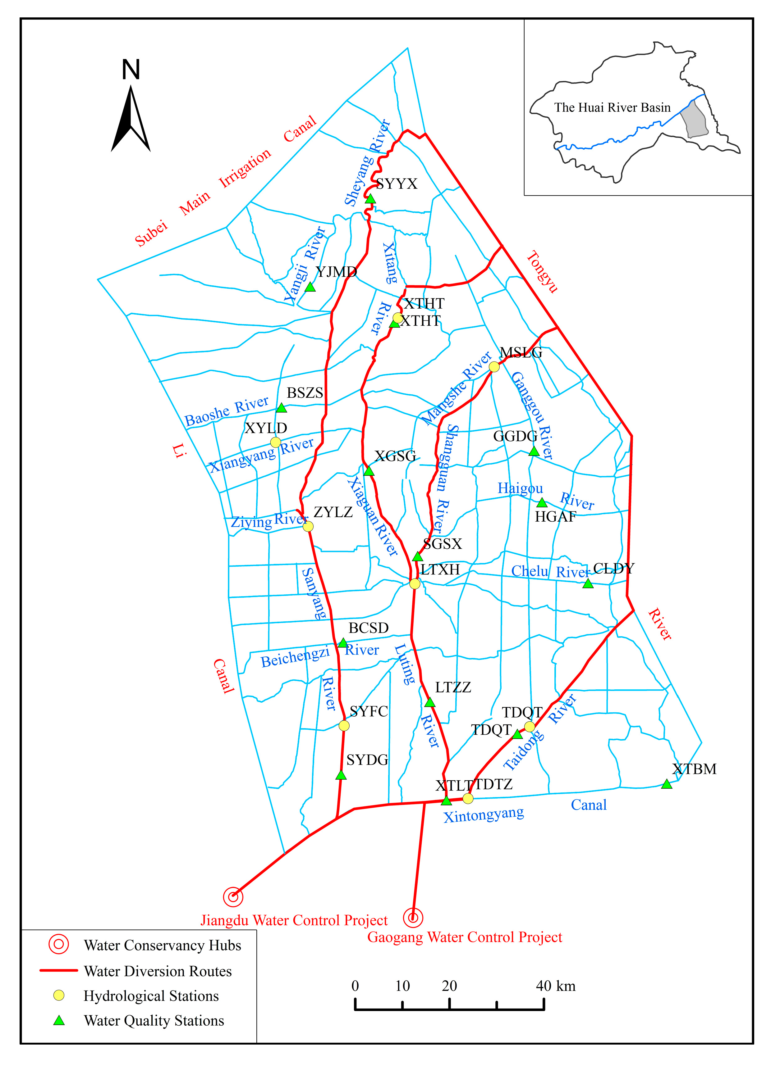
2.1. Study Area Description

The Lixiahe abdominal area is a relatively closed plain river network in the lower reaches of the Huai River in Northern Jiangsu Province, China, with an area of 11,722 km², which is located to the east of Li Canal, the south of Subei Main Irrigation Canal, the west of Tongyu River, the north of 328 National Highway from Yangzhou to Nantong, and the Rutai canal (Figure 1). There are many rivers, polder networks, lakes, marshes, and wetlands in the area. The terrain is high around, low in the middle, with an altitude ranging from 0 to 10 m above the old-yellow river datum plane. The area belongs to a subtropical monsoon climate and it is affected by a marine climate. The annual average precipitation is 1025 mm, and the precipitation in flood season accounts for about 70% of the annual rainfall.

Since it is located in the lower reaches of the Huai River, the water quality of the water from the upper reaches is generally poor. The water used in the area is mainly from the Jiangdu water conservancy project and the Gaogang water conservancy project, by which the high-quality Yangtze River water enters the area through the Xintongyang canal and the Taizhouyingjiang River to meet the demand for water for life, industry, and agriculture (Figure 1). Point source pollutant is a major pollution source, while the contribution of agricultural non-point source pollution has been growing. The mean annual load of four main water quality indicators (permanganate index: COD_Mn, ammonium nitrogen: NH₃-N, total nitrogen: TN, total phosphorus: TP) was 29,000, 10,000, 23,000, and 7000 tons in 2003–2017.

2.2. Hydrological and Water Quality Monitoring

In this study, the monthly water quality data of 15 monitoring stations and the daily water level data of 8 hydrological stations were collected from 2003 to 2017. The monitoring stations cover Taizhou, Yancheng, and Yangzhou, which are three important areas in the Lixiahe abdominal area (Figure 1). The data were collected by the Taizhou Branch, Yancheng branch, and Yangzhou Branch of the Jiangsu Bureau of the hydrological and water resources survey. In addition, daily water diversion data of Gaogang and Jiangdu station from 2003 to 2017 were collected from the Taizhou and Yangzhou Branch of the Jiangsu hydrological and Water Resources Survey Bureau.

2.3. Research Methods

Two main water quality indicators, permanganate index (COD_Mn) and ammonia nitrogen (NH₃-N), are selected for analysis, and the comprehensive water quality index (CWQI) determined by these two factors is calculated. The long-term trend of water quality is studied by using methods of continuous wavelet transform, Mann–Kendall trend test, and Sen’s slope estimator. The correlation between water quality and water level as well as water diversion volume are investigated by cross wavelet transform and wavelet coherence analysis.

2.3.1. Comprehensive Water Quality Identification Index (CWQI)

The comprehensive water quality index comprehensively takes into account a variety of pollution indexes, which can fully express the overall comprehensive water quality information of the river. The CWQI is computed using the formula of Xu [33].

$$I_{wq}=X_1·X_2=\frac{1}{m}{\displaystyle \sum }(P_1+P_2+\cdots +P_m)$$

(1)

where X₁ represents the overall water quality grade in the water quality category, X₂ represents the position of the water quality within the same grade, m is the number of water quality indexes participating in the comprehensive water quality evaluation, and P₁, P₂ and P_m represent the single factor water quality identification index (SWQI) of different monitoring items. The calculation of SWQI follows the method of Xu [7],

$$P_i=X_1·X_2$$

(2)

where X₁ equals grade value of water quality, and X₂ reads

$$X_2=\frac{{\rho }_i-{\rho }_{ikl}}{{\rho }_{iku}-{\rho }_{ikl}}$$

(3)

where ${\rho }_i$ is the measured mass concentration, k equals X₁, and ${\rho }_{ikl}$ and ${\rho }_{iku}$ are the lower and upper limit value of grade k for monitoring item i. The advantage of SWQI compared to pollutant concentration is that the measured values of different indicators can be converted into the values corresponding to the water quality category.

The water quality category used in this study is the Standard for surface water environmental quality assessment of China (GB3838-2002) [34]. The detailed range values of water quality indicators and SWQI/CWQI corresponding to different water quality grades as well as its description are presented in

Table 1. The range values of water quality category.

Indicator	Range Values (mg/L)
	Grade I	Grade II	Grade III	Grade IV	Grade V	Inferior to Grade V
CODMn	[0, 2)	[2, 4)	[4, 6)	[6, 10)	[10, 15)	[15, infinity)
NH3-N	[0, 0.15)	[0.15, 0.5)	[0.5, 1)	[1, 1.5)	[1.5, 2)	[2, infinity)
SWQI/CWQI	[1, 2)	[2, 3)	[3, 4)	[4, 5)	[5, 6)	[6, infinity)
Description	Extremely good	Very good	Good	Poor	Very poor	Extremely poor

Note: The range values of COD_Mn and NH₃-N are cited from (GB3838-2002) [34].

, where the range values of single indicators are according to GB3838-2002 [34], the range values of SWQI/CWQI are according to the calculation method introduced by Xu [7,33], and the water quality description is subjectively given according to the regional water quality objective of Grade III.

2.3.2. Continuous Wavelet Transform

Continuous wavelet analysis can clearly reveal a variety of variation periods hidden in the time series by decomposing a time series into time–frequency space. The time series of CWQI is standardized, and the significant period CWQI variation is analyzed by using the continuous wavelet transform (CWT) method. The CWT used in this work followed the method of Torrence and Compo [20,35], and the Morlet wavelet was employed as the mother function for the analysis. The prototype formula of Morlet is

$${\mathsf{\Psi }}_0\left(\eta \right)={\pi }^{-1/4}{e}^{i{\omega }_0\eta }{e}^{-{\eta }^2/2}$$

(4)

where $\eta$ is dimensionless time, and ${\omega }_0$ is a dimensionless frequency, which can be set to 6 to satisfy the admissible condition. The CWT of the discrete time series x_n is defined as

$$W_n^X\left(s\right)={\displaystyle \sum }_{n^{\prime }=0}^{N-1}{x}_{n^{\prime }}{\mathsf{\Psi }}^{*}\left[\left(n^{\prime }-n\right)\frac{\delta t}{s}\right]$$

(5)

where $W_n^X\left(s\right)$ is the wavelet coefficients, N is the length of the time series x_n, * is the complex conjugate, and $\delta t$ is the temporal sampling interval.${\left|W_n\left(s\right)\right|}^2$ represents the wavelet power spectrum. By varying the wavelet scale s and translating along the localized time index n, the wavelet power spectrum reveals the fluctuating energy of different periodicities defined by s versus time.

Red noise is used as background spectrum to test the wavelet spectrum. The first order autoregressive (AR1) process is used in the red noise test. The power spectrum of background red noise is defined as

$$P_k=\left(1-{\alpha }_2\right)/\left(\left|1-{\alpha }_2{e}^{-2i\pi k}\right|\right)$$

(6)

where $\alpha$ is the correlation coefficient of autoregressive equation in red noise power spectrum, and k is the Fourier frequency index. In general, values outside the wavelet influence cone (COI) at various scales are estimated at the significance level of 5%. For detailed information, please refer to references [20,21]. In this study, cross wavelet transform (XWT) and wavelet coherence (WTC) were done in Matlab software.

2.3.3. Trend Analysis Methods

Tests for the detection of significant trends in a hydro-meteorological time series can be classified as parametric and non-parametric methods. Parametric trend tests require data to be independent and normally distributed, while non-parametric trend tests require only that the data be independent [36]. In this study, two non-parametric methods (Mann–Kendall trend test and Sen’s slope estimator) were used to detect the trends of water quality indicators. The Mann–Kendall statistical test is able to quantify the significance of trends in time series, and the Sen’s slope estimator is used for estimating the slope of trend, both of which are widely used in hydro-meteorological time series [37,38].

In the Mann–Kendall statistical test, the standard normal test statistic Z_S is computed according to reference [36]. Positive values of Z_S indicate increasing trends, while negative Z_S values show decreasing trends. Testing trends is done at the significance level $\alpha =0.05$.

When $\left|{\mathrm{Z}}_{\mathrm{s}}\right|>{\mathrm{Z}}_{1-\alpha }$, α significant trend exists in the time series, where ${\mathrm{Z}}_{1-\alpha }=1.96$. In the Sen’s slope estimator, Q_med is computed, the sign of which reflects data trend reflection, while the value of which indicates the steepness of the trend. For detailed information on the Mann–Kendall and Sen’s slope estimator, please refer to references [36,39].

2.3.4. Cross Wavelet Transform and Wavelet Coherence

Cross wavelet transform (XWT) and wavelet coherence (WTC) can reveal the multi-scale relationship between two time series in the time-frequency domain, and they can analyze the resonance period and phase relationship in high-energy and low-energy regions, respectively [21]. In this study, XWT and WTC methods are used to analyze the relationship between water quality variation and water level and water diversion volume, and the methods follow Grinsted et al. [21].

The result of the XWT of two series X_n and Y_n is defined as

$$W_n^{XY}=W_n^X{W}_n^{Y^{*}}$$

(7)

where $\left|W^{XY}\right|$ is the cross wavelet power, and * is the complex conjugate.

The WTC is defined as

$$R_n^2\left(s\right)=\frac{{\left|S\left(s^{-1}{W}_n^{XY}\left(s\right)\right)\right|}^2}{S\left(s^{-1}{\left|W_n^X\left(s\right)\right|}^2\right)·S\left(s^{-1}{\left|W_n^Y\left(s\right)\right|}^2\right)}$$

(8)

where s is a smoothing operator. The level of statistical significance of WTC was estimated using the Monte Carlo method. For detailed information, please refer to references [20,21]. In this study, XWT and WTC were done in Matlab software.

3. Characteristics of Water Quality Variation

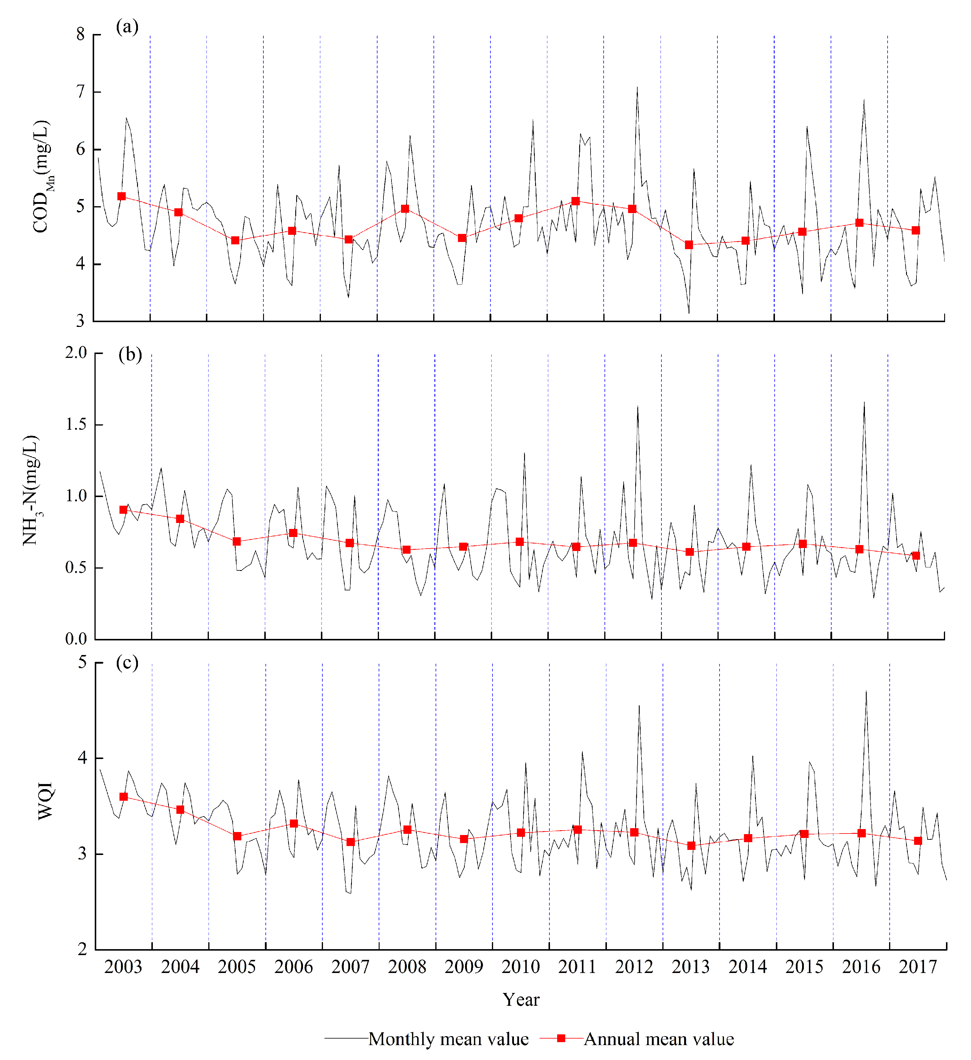
3.1. General Description of Water Quality

During 2003–2017, the annual mean COD_Mn and NH₃-N in the Lixiahe abdominal area are 4.69 mg/L and 0.68 mg/L, and the CWQI is 3.24, which is Grade III according to GB3838-2002 [34]. According to the results of the Mann–Kendall trend test and Sen’s slope estimator on water quality indicators, NH₃-N and CWQI show a significant decreasing trend (

Table 2. Trend analysis of regional annual mean COD_Mn, NH₃-N, and CWQI.

Indicator	Zs Value	Trend Slope	Tendency	Significance
CODMn	−0.693	−0.015	Decrease	Not significant
NH3-N	−3.068	−0.01	Decrease	Significant
CWQI	−1.98	−0.013	Decrease	Significant

). Hence, the water quality improves (Figure 2).

The regional water quality shows significant seasonal changes (Figure 2). From January to March, COD_Mn and NH₃-N are both high; from April to June, COD_Mn and NH₃-N are gradually decreasing, and the water quality is gradually improving; in July, COD_Mn and NH₃-N are both soaring, and the water quality is the worst in the year; from August to October, COD_Mn and NH₃-N are gradually decreasing, and the water quality is gradually improving; from November to December, the NH₃-N increases, and the water quality is slightly worse (

Table 3. Intra-annual variation of water quality.

Month	January	February	March	April	May	June	July	August	September	October	November	December	Mean	Standard Deviation
CODMn (mg/L)	4.9	4.8	4.8	4.5	4.0	4.1	5.6	5.2	5.0	4.6	4.5	4.4	4.7	0.68
NH3-N (mg/L)	0.80	0.85	0.77	0.69	0.59	0.54	1.04	0.64	0.52	0.55	0.62	0.61	0.68	0.24
CWQI	3.35	3.42	3.36	3.19	3.00	2.96	3.80	3.34	3.15	3.09	3.16	3.10	3.24	0.35

). The seasonal variation of water quality is mainly affected by the rainfall and the amount of water diversion. From January to May, the water quality gradually improves with the increase of water diversion volume; from June to September, the water diversion volume gradually decreases, and the precipitation rises to the maximum value in the year, which brings a large amount of non-point source pollutants to rivers, resulting in the deterioration of the water body; from October to December, the precipitation is low, but the water diversion volume increases significantly, and the water quality improves [40].

There is significant spatial variation in the water quality. The COD_Mn and NH₃-N of YJMD in the northwest and SYYX, LTZZ, SYDG, TDQT, XTLT in the main river channels of water diversion are relatively low, and the water quality is very good, with CWQI smaller than 3. The NH₃-N of SGSX is high, and the COD_Mn of GGDG, XTHT, CLDY, HGAF, XGSG is high, and the water quality is good, with CWQI in the range of 3–4. At BCSD, BSZS and XTBM, both COD_Mn and NH₃-N are high, with a CWQI larger than 4; therefore, the water quality is poor (Table 3). The regional water quality target is Grade III of GB3838-2002, but the COD_Mn and NH₃-N of each station exceed the standard by a certain proportion, with regional mean overproof rates of 15% and 21%, respectively. Here, the overproof rate means the portion of observed water quality data inferior to Grade III, whose upper limit value of COD_Mn and NH₃-N is 6 mg/L and 1 mg/L, respectively [19]. The overproof rates of COD_Mn at BSZS, XGSG and XTBM are high, with values bigger than 20%. The overproof rates of NH₃-N at XTBM, BCSD, BSZS, SGSX and XTLT are high, with values bigger than 25% (

Table 4. Characteristic values of annual mean water quality of each station.

Region	Monitoring Stations	CODMn (mg/L)				NH3-N (mg/L)				CWQI
		Max.	Min.	Mean	op Rate * (%)	Max.	Min.	Mean	op Rate * (%)	Max.	Min.	Mean
Taizhou	CLDY	6.0	2.5	4.9	16	1.0	0.3	0.5	9	3.7	2.7	3.2
	HGAF	6.1	1.8	5.1	18	1.0	0.2	0.5	7	3.8	1.8	3.2
	LTZZ	4.5	2.0	3.6	6	0.8	0.2	0.5	10	3.3	2.3	2.8
	SGSX	5.8	2.8	4.6	8	1.3	0.5	0.9	32	3.9	3.0	3.5
	TDQT	4.8	1.8	3.4	3	1.1	0.3	0.6	16	3.6	2.1	2.9
	XGSG	8.1	4.8	5.7	28	1.0	0.3	0.6	10	4.1	3.2	3.4
	XTBM	6.7	2.0	5.0	24	2.4	0.3	1.6	73	4.9	2.2	4.2
	XTLT	5.0	3.0	3.5	6	1.1	0.3	0.7	25	3.7	2.5	3.0
Yancheng	GGDG	5.6	4.8	5.3	13	0.7	0.2	0.4	4	3.4	2.9	3.1
	SYYX	5.2	4.4	4.7	4	0.4	0.1	0.3	2	3.0	2.5	2.8
	XTHT	9.3	4.5	5.2	17	0.7	0.3	0.4	2	3.9	2.8	3.1
	YJMD	5.4	3.6	4.4	5	1.4	0.1	0.3	7	3.9	2.1	2.7
Yangzhou	BSZS	8.0	4.4	6.1	42	2.2	0.9	1.1	49	5.0	3.5	4.0
	BCSD	7.4	4.2	5.0	18	1.9	1.0	1.4	62	4.6	3.6	4.0
	SYDG	6.5	2.9	3.9	8	0.7	0.2	0.5	7	3.6	2.3	2.8

* overproof rate: portion of observed water quality data inferior to Grade III.

).

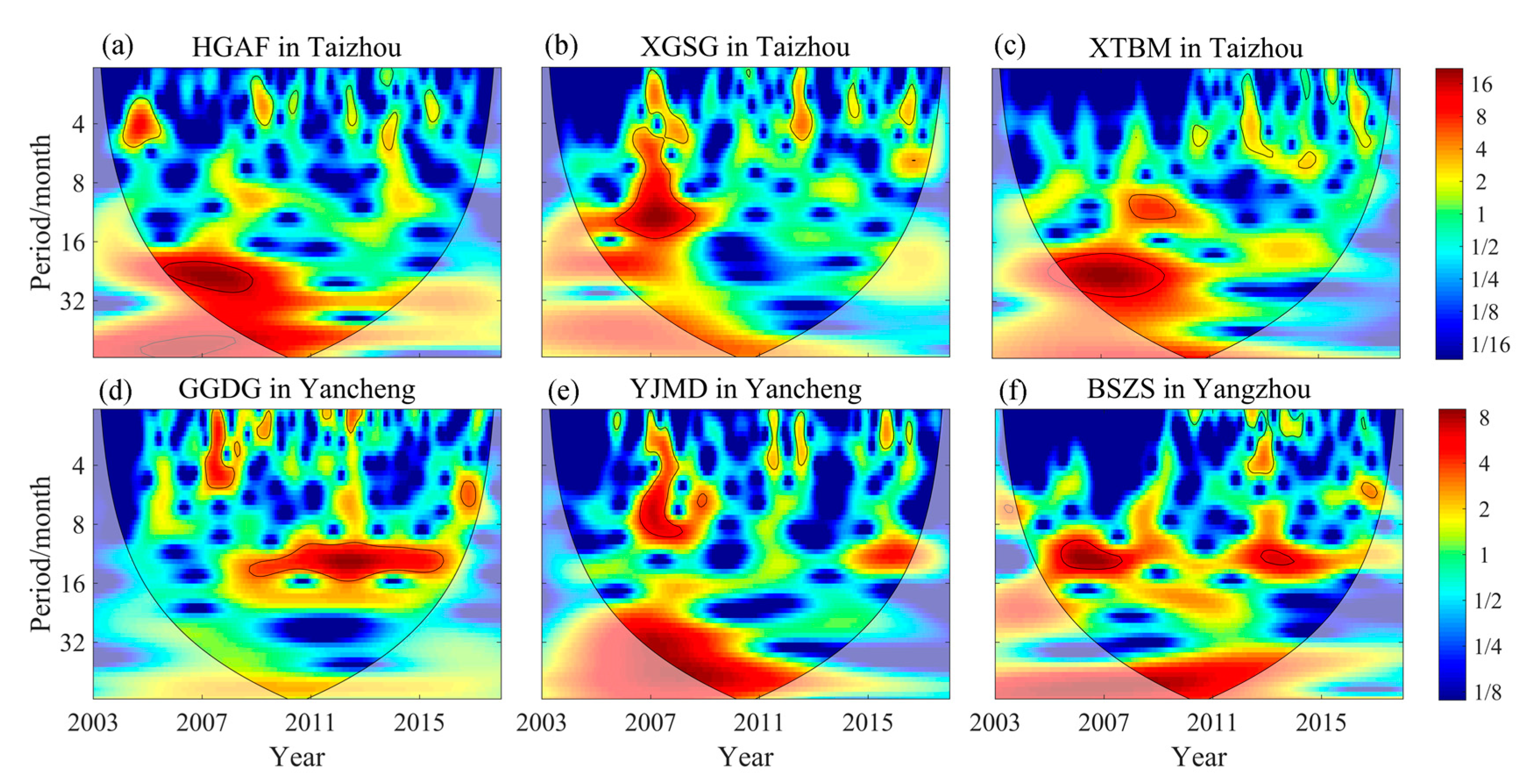
3.2. Periodic Variation of Water Quality

CWT was employed to the CWQI time series of each station to analyze its periodic characteristics. The CWT results of some stations are presented in Figure 3, and the characteristic period of each station is summarized in

Table 5. The characteristic periods of CWQI.

Region	Monitoring Stations	Characteristic Periods
Taizhou	CLDY	Time	2010–2012	2012–2013	2015	-	-
		Period (month)	10–13	2–5	2–4	-	-
	HGAF	Time	2004–2005	2005–2008	2008–2009	2013–2014	2016
		Period (month)	2–6	21–30	2–4	4–6	2–4
	LTZZ	Time	2005–2007	2010–2012	2012	2012–2013	2016–2017
		Period (month)	18–25	10–15	2–5	6–7	2–6
	SGSX	Time	2007–2009	2008–2010	2012–2013	2016–2017	-
		Period (month)	5–7	9–14	6	2–8	-
	TDQT	Time	2005–2008	2007–2008	2010–2011	2015	2016
		Period (month)	21–30	5–7	6–7	4–5	2–7
	XGSG	Time	2005–2008	2006–2008	2012	2014	2016
		Period (month)	4–16	2–5	2–5	2–4	2–4
	XTBM	Time	2005–2009	2007–2009	2012–2013	2014	2015–2016
		Period (month)	18–31	9–13	2–6	5–7	2–5
	XTLT	Time	2005–2007	2013	2016	-	-
		Period (month)	2–8	2–3	2–4	-	-
Yancheng	GGDG	Time	2007–2008	2008–2015	2016–2017	-	-
		Period (month)	2–6	10–16	6–7	-	-
	SYYX	Time	2007	2008–2009	2015–2016	2016	-
		Period (month)	2–5	6–7	9–14	4–6	-
	XTHT	Time	2006–2008	2012	2015–2016	-	-
		Period (month)	30–36	2–4	2–5	-	-
	YJMD	Time	2006–2007	2008	2011	-	-
		Period (month)	2–10	6–7	2–4	-	-
Yangzhou	BSZS	Time	2005–2007	2012–2013	2012–2013	2016	-
		Period (month)	10–15	2–5	11–15	5–6	-
	BCSD	Time	2003–2005	2007	2009–2010	2010–2012	2012–2013
		Period (month)	4–9	13	6–8	46–59	2–5
	SYDG	Time	2003–2004	2005–2006	2007–2008	2011	2016
		Period (month)	6–7	4–7	6–7	7	2–6

. At a 95% confidence level, the CWQI of each station has a significant period in the time-frequency domain.

In northern Taizhou, CLDY, SGSX, and XGSG have a period of 10–12 months, and the periodic occurrence of each station is different; HGAF has a period of 21–30 months (2005–2008). In southern Taizhou, LTZZ, TDQT, and XTBM have a period of 21–25 months (2005–2008), and XTLT has a period of 2–8 months (2005–2007). In the Yancheng area, GGDG, SYYX, and YJMD have a period of 10 months, and the periods of occurrence of each station are different. XTHT has a period of 30–36 months (2006–2008). In the Yangzhou area, BSZS and SYDG have a 13-month cycle (2005–2007); SYDG has a 4–7-month cycle (2005–2006). In general, the CWQI of each station contains multi-scale significant periodic fluctuations of 3–59 months, and the seasonal variation of 12 months is significant at most stations.

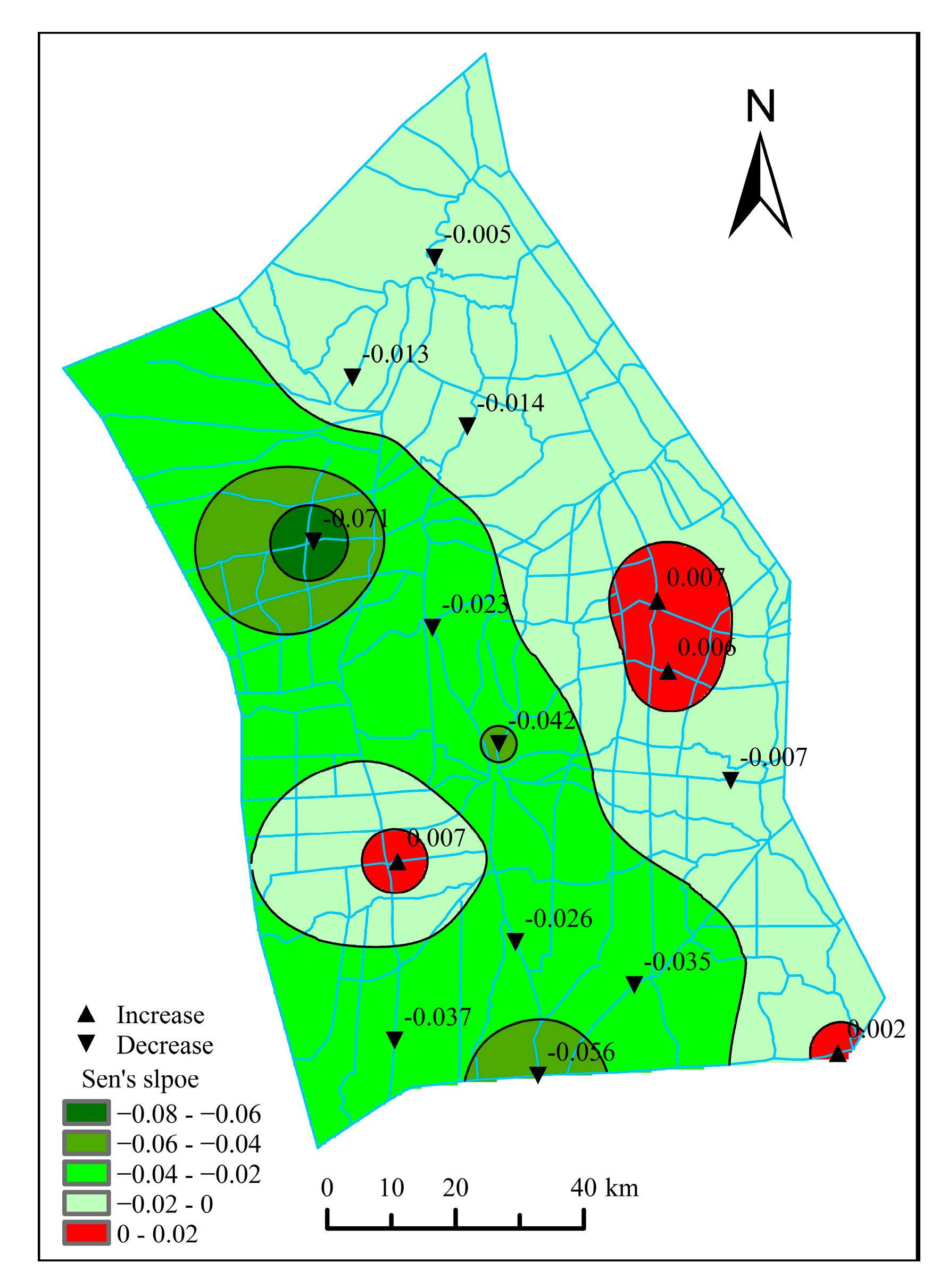
3.3. Long-Term Trends of Water Quality

Long-term trends of water quality were investigated by applying the Mann–Kendall trend test and Sen’s slope estimator on the CWQI. The CWQI of 7 out of 15 monitoring stations has a significant decreasing trend (

Table 6. The trend and trend slope of the CWQI.

Region	Monitoring Stations	Zs Value	Annual Trend Slope	Tendency	Significance
Taizhou	CLDY	−0.897	−0.007	Decrease	Not significant
	HGAF	0.739	0.006	Increase	Not significant
	LTZZ	−2.734	−0.026	Decrease	Significant
	SGSX	−4.267	−0.042	Decrease	Significant
	TDQT	−2.985	−0.035	Decrease	Significant
	XGSG	−3.144	−0.023	Decrease	Significant
	XTBM	0.170	0.002	Increase	Not significant
	XTLT	−4.015	−0.056	Decrease	Significant
Yancheng	GGDG	0.964	0.007	Increase	Not significant
	SYYX	−0.685	−0.005	Decrease	Not significant
	STHT	−1.851	−0.014	Decrease	Not significant
	YJMD	−1.549	−0.013	Decrease	Not significant
Yangzhou	BSZS	−6.245	−0.071	Decrease	Significant
	BCSD	0.510	0.007	Increase	Not significant
	SYDG	−2.854	−0.037	Decrease	Significant

). In the Taizhou area, the trend of the CWQI of XTLT is the most significant, showing a rapid decreasing trend, with a trend slope to be −0.056/yr, and the water quality is greatly improved; at SGSX, TDQT, LTZZ, and XGSG, the CWQI variation shows a very significant decreasing trend, with the trend slope to be between −0.046/yr and −0.023/yr, and the water quality is significantly improved. The CWQI variation of CLDY, HGAF, and XTBM is not significant. In the Yancheng area, the trend of CWQI variation is not significant. In the Yangzhou area, the trend of CWQI of BSZS is the most significant, showing a rapid decreasing trend, with the trend slope to be −0.071/yr, which indicates the water quality improvement by one grade in 15 years, and the water quality is greatly improved. The CWQI of SYDG shows a very significant decreasing trend, with the trend slope to be −0.037/yr, and the water quality is obviously improved. The CWQI variation of BCSD is not significant.

The trend slope of CWQI ranges from −0.071/yr to 0.007/yr, and two-thirds of the monitoring stations have a negative trend slope, indicating that the water quality of rivers in the Lixiahe abdominal area is gradually improving, but the spatial difference is large (Figure 4). The water quality of XTLT, TDQT, SGSX, LTZZ, and XGSG in the Taizhou area and SYDG and BSZS in the Yangzhou area, which are located in the main channels of water diversion, has been significantly improved, while in the Yancheng area, which is located downstream of the water diversion, the improvement on water quality is not significant. The water quality of the XTBM in the southeastern area, HGAF and GGDG in the eastern area, and BCSD in the western area, which cannot be reached by the diversion water, even shows a trend of deterioration.

4. Possible Causes of Water Quality Variation

The temporal and spatial variation of water quality is closely related to the discharge and accumulation of pollutants, the local water resources from precipitation, and the amount of water from external sources. Therefore, the following discussion focuses on the impact of water pollutant input, water level, and the amount of diversion water on water quality.

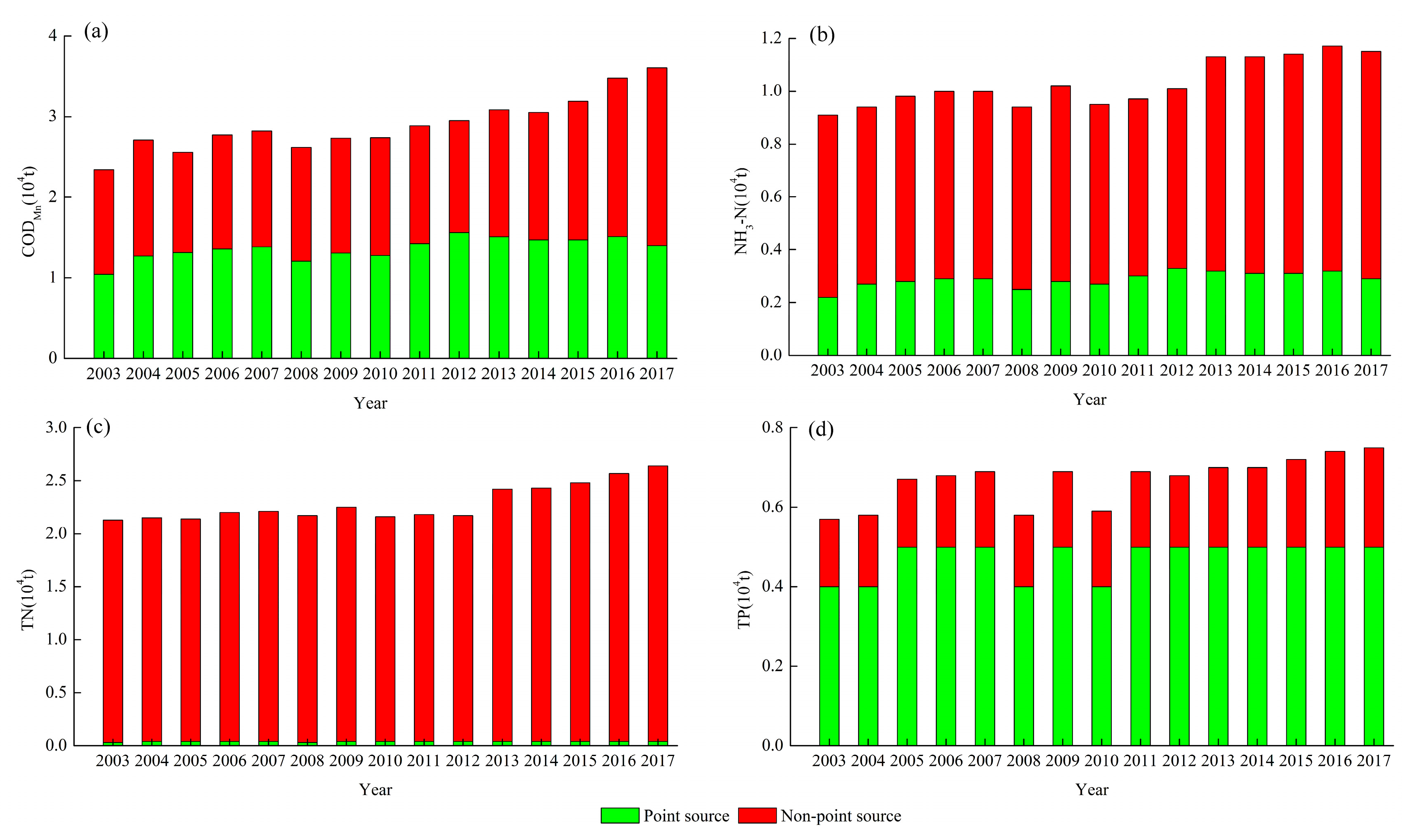
4.1. Input of Regional Water Pollutants

It is not easy to obtain the regional short-term pollutant input; thus, the annual load of four main indicators (COD_Mn, NH₃-N, TN, and TP) of the Lixiahe abdominal area was calculated according to the Jiangsu Statistical Yearbook (Figure 5). During 2003–2017, the discharge of COD_Mn and TP increased by 54% and 39% respectively, while the increase in NH₃-N and TN was slightly smaller, 27% and 24%. The growth rate of point source pollutants from industrial and municipal wastewater emissions is about 35%. The main point source pollutant inputs are COD_Mn and TP, and the amount of NH₃-N and TN is relatively small. Among the non-point source pollutants, the growth rate of COD_Mn and TP is relatively large, 70% and 47% respectively, and the growth rate of NH₃-N and TN is relatively small, about 24%. In general, with the booming of the social economy, the main pollutants discharged to river water have increased significantly, which may induce water environment deterioration.

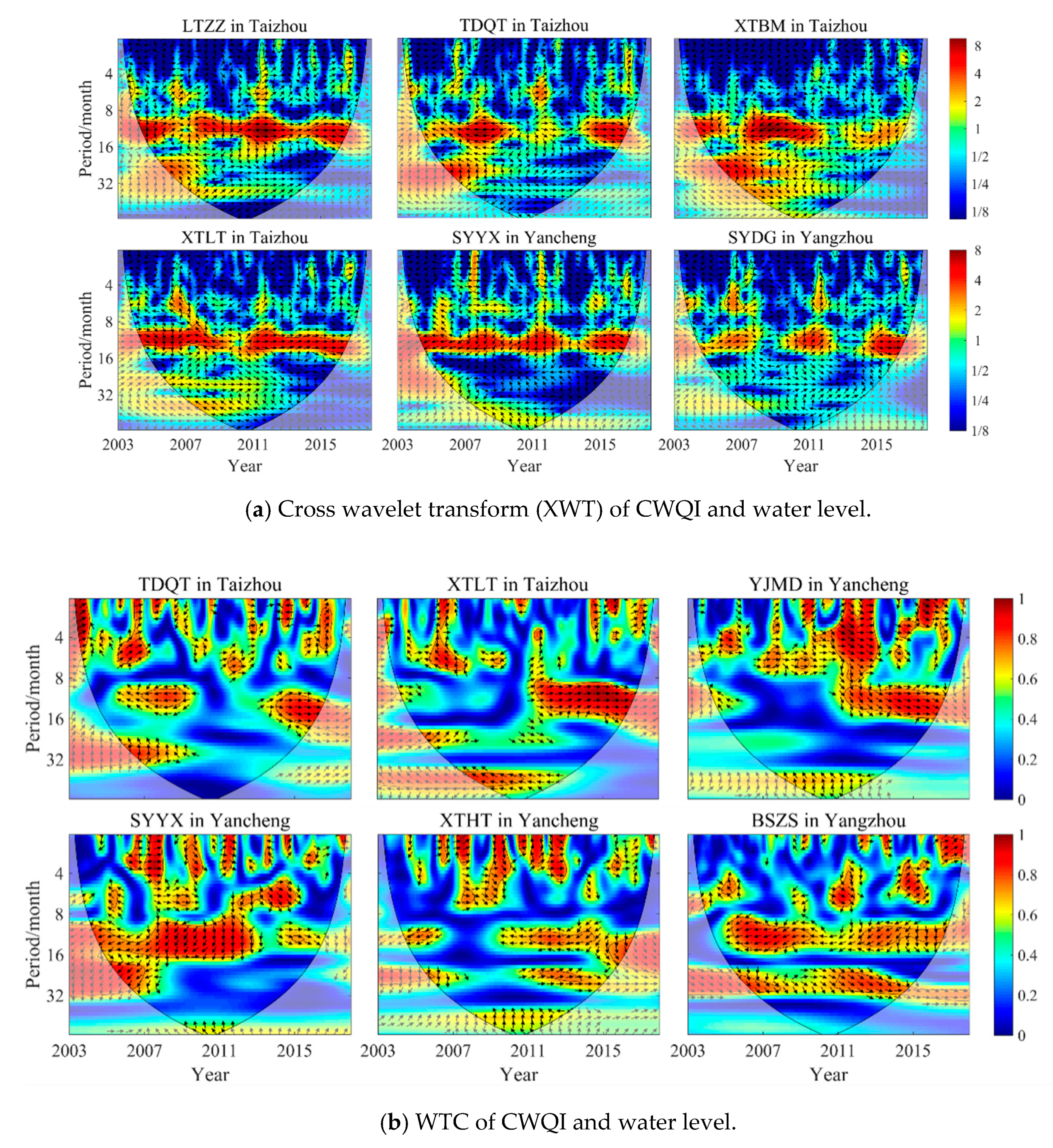
4.2. Correlation Analysis of Water Quality and Water Level

The water level reflects the amount of water in the area, which is influenced by multi-processes of precipitation, water diversion, and drainage, and it has an important impact on the water quality. The correlation of the CWQI and water level of each station are analyzed by XWT and WTC analysis by identifying the resonance period. The XWT and WTC reflect the resonance signal characteristics and the correlation coefficient of the CWQI and water level in the high-energy area and low-energy area, respectively. The results of XWT and WTC analysis at some stations are shown in Figure 6, and the correlation between the CWQI and water level at each station is summarized in

Table 7. Correlation between the CWQI and water level.

Region	Monitoring Stations	High-Energy Area			Low-Energy Area
		Resonance Period (Month)	Time	Phase Relationship	Resonance Period (Month)	Time	Phase Relationship	Correlation Coefficient
Taizhou	CLDY	10–14	2009–2013	→	4–7	2005–2007	↑	0.8
		10–14	2013–2016	→	8–16	2010–2015	→	0.8
	HGAF	11–13	2008	←	1–4	2016–2017	↑	0.9
	LTZZ	10–14	2004–2006	↑	4–7	2006–2007	→	0.8
		9–15	2007–2013	→	39–50	2007–2012	→	0.7
		11–14	2014–2016	→	8–20	2011–2016	→	0.9
	SGSX	10–14	2007–2011	←	2–6	2011	→	0.8
		-	-	-	10–14	2012–2015	→	0.7
	TDQT	10–15	2006–2009	←	10–13	2007–2009	←	0.7
		11–15	2014–2016	→	27–32	2005–2007	↑	0.8
		-	-	-	12–26	2013–2016	→	0.9
	XGSG	9–16	2004–2009	←	10–16	2005–2009	←	0.8
		-	-	-	43–57	2007–2009	←	0.7
	XTBM	10–13	2004–2005	→	8–16	2008–2010	←	0.8
		9–15	2007–2011	→	-	-	-	-
	XTLT	9–14	2004–2008	↓	40–52	2007–2010	←	0.7
		10–15	2010–2016	→	8–16	2011–2016	→	0.9
Yancheng	GGDG	10–15	2009–2013	→	2–8	2004–2006	→	0.9
		12–14	2013–2016	→	8–14	2008–2013	→	0.8
	SYYX	11–15	2004–2009	←	20–30	2005–2006	←	0.8
		10–15	2009–2012	↓	9–18	2004–2012	←	0.9
		11–14	2014–2016	→	-	-	-	-
	XTHT	11–14	2004–2006	←	12–13	2004–2005	←	0.7
		12–14	2008–2010	←	12–14	2011–2014	←	0.7
		-	-	-	12–20	2015–2016	↓	0.8
	YJMD	12–14	2014–2016	→	1–9	2009–2012	→	0.9
		-	-	-	10–16	2011–2016	→	0.8
Yangzhou	BSZS	9–15	2004–2009	←	8–15	2005–2009	←	0.9
		11–14	2011–2015	←	21–31	2011–2014	→	0.8
		-	-	-	11–14	2012–2016	←	0.8
	BCSD	9–15	2004–2010	←	9–16	2004–2012	←	0.9
	SYDG	11–13	2010–2011	→	1–6	2005–2007	↑	0.9
		12–15	2014–2016	→	12–15	2015–2016	→	0.8

.

In the Taizhou area, except for HGAF, the CWQI and water level of the other seven stations have a resonance period of 12–14 months, CLDY, LTZZ, and XTLT have positive correlations, XGSG and XTBM have negative correlations, SGSX has negative and positive correlations in the high-energy area and low-energy area respectively, TDQT has a transition from negative correlation to positive correlation in the high-energy area and positive correlation in the low-energy area. In the Yancheng area, there is a 12–14-month resonance period between the CWQI and water level at four monitoring stations, GGDG and YJMD have positive correlations, XTHT has a negative correlation, SYYX has positive and negative correlations in the high-energy area and low-energy area, respectively. In the Yangzhou area, there are 12–14-month resonance periods between the CWQI and water level of three monitoring stations, BSZS and BCSD have a negative correlation, and SYDG has a positive correlation.

In general, the CWQI has a resonance period of about 12 months with water level, with positive correlation accounting for 62% and negative correlation accounting for 38%. The change of correlation in different periods is mainly related to the water level being affected by multiple factors, such as local water resources, water diversion, and drainage. The increase in local water recourse due to precipitation induces the water level rise and water quality deterioration with an increase in the CWQI, due to large amount of non-point source pollutants entering the river with rainfall runoff. The increase in diversion water leads to water level rise and water quality improvement with an increase in the CWQI. Hence, the CWQI and water level is mainly negatively correlated in the wet season, when the water resource is mainly from rainfall runoff, while the CWQI and water level is mainly positively correlated in the dry season, when the water resource is mainly from water diversion.

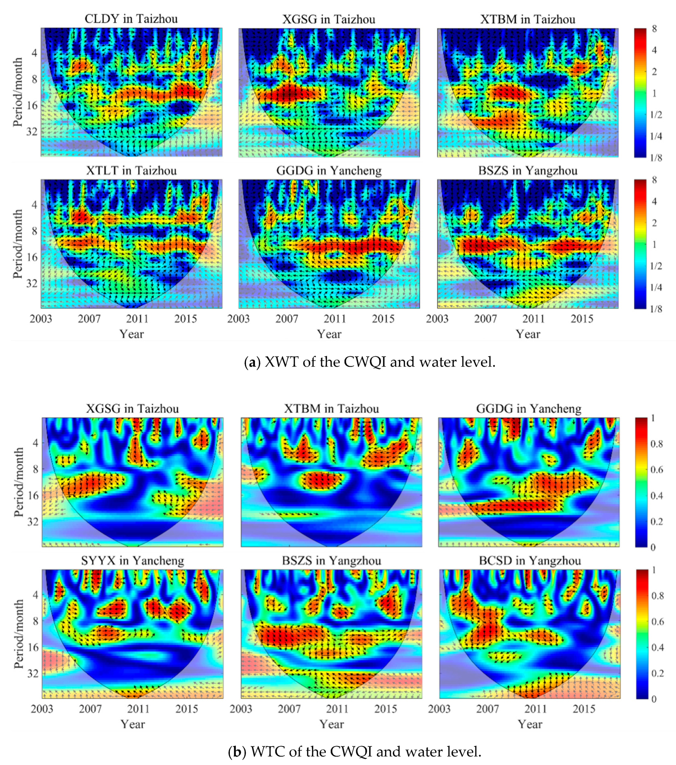
4.3. Correlation Analysis of Water Quality and Amount of Diversion Water

The Lixiahe abdominal area is in the upstream section of south-to-north water diversion from the Yangtze River in Jiangsu Province. Thus, the water quality of the area is improved by introducing the good-quality Yangtze River water. The correlation of the CWQI and water diversion volume of each station is analyzed by XWT and WTC analysis, by identifying the resonance period. The results of XWT and WTC analysis of the CWQI and water diversion volume at some stations are shown in Figure 7. The correlation between the CWQI and diversion water at each station is summarized in

Table 8. Correlation between the CWQI and the amount of diversion water.

Region	Monitoring Stations	High-Energy Region			Low-Energy Region
		Resonance Period (Month)	Time	Phase Relationship	Resonance Period (Month)	Time	Phase Relationship	Correlation Coefficient
Taizhou	CLDY	10–13	2013–2015	←	1–7	2004–2007	←	0.9
		-	-	-	8–16	2011–2015	←	0.8
	HGAF	5–7	2013–2014	↑	8–16	2012–2015	←	0.8
	LTZZ	12–14	2011–2012	←	3–7	2005–2008	←	0.9
		11–15	2015–2016	←	5–8	2009–2013	←	0.9
		-	-	-	11–32	2014–2016	←	0.8
		-	-	-	2–7	2015–2016	←	0.8
	SGSX	11–14	2008–2010	↓	4–7	2007–2011	←	0.9
		-	-	-	11–15	2008–2010	↓	0.7
		-	-	-	11–25	2012–2016	←	0.9
	TDQT	12–13	2007–2008	↓	4-8	2005–2007	←	0.9
		2–7	2014–2016	←	4–31	2007–2016	←	0.9
		12–14	2015–2016	←	-	-	-	-
	XGSG	10–15	2005–2008	↓	10–16	2004–2008	↓	0.8
	XTBM	10–13	2007–2009	→	9–14	2008–2011	→	0.9
		-	-	-	4–8	2013–2016	←	0.8
	XTLT	4–7	2005–2007	←	1–8	2004–2013	←	0.9
		11–12	2005–2007	→	10–18	2012–2016	←	0.9
		12–15	2015–2016	←	-	-	-	-
Yancheng	GGDG	11–16	2008–2016	←	10–16	2010–2014	↑	0.8
		-	-	-	18–27	2005–2012	←	0.9
	SYYX	11-14	2014–2016	←	5–8	2007–2009	←	0.9
		-	-	-	10–14	2007–2009	→	0.8
		-	-	-	5–8	2013–2014	←	0.9
	XTHT	12–14	2009–2010	→	11–14	2004–2005	→	0.8
		-	-	-	11–16	2009–2011	→	0.7
		-	-	-	10–13	2013–2014	→	0.7
	YJMD	12–14	2014–2016	←	4–7	2008–2010	←	0.9
		-	-	-	9–15	2012–2016	←	0.8
Yangzhou	BSZS	11–14	2005–2008	→	10–16	2004–2009	→	0.9
		12–14	2012–2014	→	12–16	2012–2013	→	0.7
	BCSD	4–8	2004–2006	←	1–15	2003–2007	←	0.9
		12–14	2005–2008	↓	12–14	2010–2012	→	0.7
	SYDG	4–7	2005–2007	←	1–8	2004–2009	←	0.9
		2–7	2014–2016	←	2–8	2010–2014	←	0.9
		12–15	2015–2016	←	2–15	2014–2016	←	0.8

.

In the Taizhou area, except for the high-energy area of HGAF, there is a resonance period of 11–12 months for the CWQI and water diversion volume of each station; CLDY, HGAF, LTZZ, SGSX and TDQT have inverse correlation, the CWQI of XGSG lags behind the water diversion volume by one-quarter of a cycle, while XTBM and XTLT have different correlation in the high-energy area and low-energy area. In the Yancheng area, there is a 12–13-month resonance period between the CWQI and water diversion volume at four monitoring stations. Here, XTHT has positive correlation, GGDG and YJMD have negative correlation, SYYX has different correlations in the high-energy area and low-energy area. In the Yangzhou area, the resonance period of the CWQI and water diversion volume of three monitoring stations is 12–14 months, BSZS has a positive correlation, SYDG has a negative correlation, and the CWQI of BCSD lags behind the water diversion volume by one-quarter of a cycle.

In general, there is a resonance period of about 12 months between the CWQI and water diversion volume at each monitoring station. Two-thirds of the 15 monitoring stations are located in the main channels of water diversion and nearby rivers, and one-third is far away from the main channels of water diversion. The CWQI of the monitoring stations at the water diversion route and its nearby river is inversely related to the water diversion volume. The larger the water diversion volume, the better the water quality. The water diversion from the Yangtze River plays an important role in improving the regional water environment.

Due to the complexity of the water quality variation and the limitation on the methodology, this study was qualitative when assessing the possible causes of water quality variation. Nevertheless, water diversion is proved to be an important contributor to improving the regional water environment. Further work is required to investigate the quantitative relationship between the water quality and intensity and duration of water diversion to provide scientific guidance on the optimization of water diversion operation.

5. Conclusions

From 2003 to 2017, the water quality variation in the Lixiahe abdominal area contains multi-scale periodic fluctuations of 3–59 months, and the seasonal variation of 12 months is significant at most stations. The CWQI of 7 out of 15 monitoring stations has a significant decreasing trend, and the trend slope ranges from −0.071/yr to 0.007/yr. The water quality of the main routes of the water diversion and the nearby rivers has significantly improved, while the water quality of rivers far away from the main routes, which is less affected by the water diversion, has no obvious improvement, or even becomes worse.

The CWQI and water level is mainly positively correlated in the wet season, when the water resource is mainly from rainfall runoff that brings many non-point pollutants, while the CWQI and water level are mainly inversely correlated in the dry season, when the water resource is mainly from water diversion from the Yangtze River. The CWQI and the water diversion volume are inversely related at monitoring stations in the main routes of water diversion and its nearby river. Hence, water diversion plays an important role in improving the regional water environment.

With the booming of the social economy in the Lixiahe abdominal area, the main pollutants discharged to river water have increased, but the water quality has generally improved, especially in the main routes of water diversion and its nearby rivers, due to the water diversion from the Yangtze River. Hence, the key to regional water environment improvement lies in the systematic control of point and non-point source pollutants and the optimization of water diversion operation.

References

1. Zhai, X.Y.; Xia, J.; Zhang, Y.Y. Integrated approach of hydrological and water quality dynamic simulation for anthropogenic disturbance assessment in the Huai River Basin, China. Sci. Total Environ. 2017, 598, 749–764. [Google Scholar] [CrossRef] [PubMed]
2. Hussein, H. The Guarani Aquifer System, highly present but not high profile: A hydropolitical analysis of transboundary groundwater governance. Environ. Sci. Policy. 2018, 83, 54–62. [Google Scholar] [CrossRef] [Green Version]
3. Odeh, T.; Mohammad, A.H.; Hussein, H.; Ismail, M.; Almomani, T. Over-pumping of groundwater in Irbid governorate, northern Jordan: A conceptual model to analyze the effects of urbanization and agricultural activities on groundwater levels and salinity. Environ. Earth Sci. 2019, 78, 40. [Google Scholar] [CrossRef] [Green Version]
4. Mohammad, A.H.; Jung, H.C.; Odeh, T.; Bhuiyan, C.; Hussein, H. Understanding the impact of droughts in the Yarmouk Basin, Jordan: Monitoring droughts through meteorological and hydrological drought indices. Arab. J. Geosci. 2018, 11, 103. [Google Scholar] [CrossRef] [Green Version]
5. Cullaj, A.; Hasko, A.; Miho, A.; Schanz, F.; Brandl, H.; Bachofen, R. The quality of Albanian natural waters and the human impact. Environ. Int. 2005, 31, 133–146. [Google Scholar] [CrossRef]
6. Bordalo, A.A.; Teixeira, R.; Wiebe, W.J. A water quality index applied to an international shared river basin: The case of the Douro River. Environ. Manag. 2006, 38, 910–920. [Google Scholar] [CrossRef]
7. Xu, Z.-X. Single factor water quality indentification index for environmental quality assessment of surface water. J. Tongji Univ. (Nat. Sci.) 2005, 33, 321–325, (In Chinese with English abstract). [Google Scholar]
8. Lermontov, A.; Yokoyama, L.; Lermontov, M.; Machado, M.A.S. River quality analysis using fuzzy water quality index: Ribeira do Iguape river watershed, Brazil. Ecol. Indic. 2009, 9, 1188–1197. [Google Scholar] [CrossRef]
9. Zhang, Y.; Guo, F.; Meng, W.; Wang, X.-Q. Water quality assessment and source identification of Daliao river basin using multivariate statistical methods. Environ. Monit. Assess. 2009, 152, 105–121. [Google Scholar] [CrossRef]
10. Hurley, T.; Sadiq, R.; Mazumder, A. Adaptation and evaluation of the Canadian Council of Ministers of the Environment Water Quality Index (CCME WQI) for use as an effective tool to characterize drinking source water quality. Water Res. 2012, 46, 3544–3552. [Google Scholar] [CrossRef]
11. Ahmed, S.; Khurshid, S.; Madan, R.; Amarah, B.A.A.; Naushad, M. Water quality assessment of shallow aquifer based on Canadian Council of Ministers of the environment index and its impact on irrigation of Mathura District, Uttar Pradesh. J. King Saud Univ. Sci. 2020, 32, 1218–1225. [Google Scholar] [CrossRef]
12. Ajorlo, M.; Abdullah, R.B.; Yusoff, M.K.; Halim, R.A.; Hanif, A.H.M.; Willms, W.D.; Ebrahimian, M. Multivariate statistical techniques for the assessment of seasonal variations in surface water quality of pasture ecosystems. Environ. Monit. Assess. 2013, 185, 8649–8658. [Google Scholar] [CrossRef] [PubMed]
13. Sojka, M.; Siepak, M.; Ziola, A.; Frankowski, M.; Murat-Blazejewska, S.; Siepak, J. Application of multivariate statistical techniques to evaluation of water quality in the Mala Welna River (Western Poland). Environ. Monit. Assess. 2008, 147, 159–170. [Google Scholar] [CrossRef] [PubMed]
14. Zhou, L.; Xu, S. Application of grey clustering method in eutrophication assessment of wetland. J. Am. Sci. 2006, 2, 53–58. [Google Scholar]
15. Wątor, K.; Kmiecik, E.; Lipiec, I. The use of principal component analysis for the assessment of the spatial variability of curative waters from the Busko-Zdrój and Solec-Zdrój region (Poland)–preliminary results. Water Supply 2018, 19, 1137–1143. [Google Scholar] [CrossRef]
16. Xia, R.; Chen, Z. Integrated water-quality assessment of the Huai River Basin in China. J. Hydrol. Eng. 2014, 20, 05014018. [Google Scholar] [CrossRef]
17. Sarkar, A.; Pandey, P. River water quality modelling using artificial neural network technique. Aquat. Procedia 2015, 4, 1070–1077. [Google Scholar] [CrossRef]
18. Hind, J.A.; Marwan, A. Assessing groundwater vulnerability in Azraq Basin area by a modified drastic Index. J. Water Resour. Prot. 2010, 2, 944–951. [Google Scholar]
19. Merchant, J.M. GIS-Based groundwater pollution hazard assessment: A critical review of the DRASTIC Model. Photograomm. Eng. Rem. Sens. 1994, 60, 1117–1127. [Google Scholar]
20. Torrence, C.; Comopo, G.P. A practical guide to wavelet analysis. Bull. Am. Meteorol. Soc. 1998, 79, 61–78. [Google Scholar] [CrossRef] [Green Version]
21. Grinsted, A.; Moore, J.C.; Jevrejeva, S. Application of the cross wavelet transform and wavelet coherence to geophysical time serial. Nonlinear Proc. Geoph. 2004, 11, 505–514. [Google Scholar] [CrossRef]
22. Smith, L.C.; Turcotte, D.L.; Isacke, B. Stream flow characterization and feature detection using a discrete wavelet transform. Hydrol. Processes. 1998, 12, 233–249. [Google Scholar] [CrossRef]
23. Labat, D. Recent advances in wavelet analyses: Part 1. A review of concepts. J. Hydrol. 2005, 314, 275–288. [Google Scholar] [CrossRef]
24. Kang, S.-J.; Lin, H. Wavelet analysis of hydrological and water quality signals in an agricultural watershed. J. Hydrol. 2007, 338, 1–14. [Google Scholar] [CrossRef]
25. Hatvani, I.G.; Clement, A.; Korponai, J.; Kern, Z.; Kovács, Z. Periodic signals of climatic variables and water quality in a river-eutrophic pond-wetland cascade ecosystem tracked by wavelet coherence analysis. Ecol. Indic. 2017, 83, 21–31. [Google Scholar] [CrossRef] [Green Version]
26. Barzegar, R.; Adamowski, J.; Moghaddam, A.A. Application of wavelet-artificial intelligence hybrid models for water quality prediction a case study in Aji-Chay River. Stoch. Environ. Res. Risk Assess. 2016, 30, 1797–1819. [Google Scholar] [CrossRef]
27. Barzegar, R.; Moghaddam, A.A.; Adamowski, J.; Ozga-Zielinski, B. Multi-step water quality forecasting using a boosting ensemble multi-wavelet extreme learning machine model. Stoch. Environ. Res. Risk Assess. 2018, 32, 799–813. [Google Scholar] [CrossRef]
28. Parmar, K.S.; Makkhan, S.J.S.; Kaushal, S. Neuro-fuzzy-wavelet hybrid approach to estimate the future trends of river water quality. Neural Comput. Appl. 2019, 31, 8463–8473. [Google Scholar] [CrossRef]
29. Najah, A.A.; EI-Shafie, A.; Karim, O.A. Water quality prediction model utilizing integrated wavelet-ANFIS model with cross-validation. Neural Comput. Appl. 2012, 21, 833–841. [Google Scholar] [CrossRef]
30. Ghassemi, F.; White, I. Inter-basin Water Transfer: Case Studies from Australia, United States, Canada, China, and India; Cambridge University Press: New York, NY, USA, 2007. [Google Scholar]
31. Zeng, Q.H.; Qin, L.H.; Li, X.Y. The potential impact of an inter-basin water transfer project on nutrients (nitrogen and phosphorous) and chlorophyll a of the receiving water system. Sci. Total Environ. 2015, 536, 675–686. [Google Scholar] [CrossRef]
32. Hoekstra, A.Y.; Mekonnen, M.M. Imported water risk: The case of the UK. Environ. Res. Lett. 2016, 11. [Google Scholar] [CrossRef]
33. Xu, Z.-X. Comprehensive water quality identification index for environmental quality assessment of surface water. J. Tongji Univ. (Nat. Sci.) 2005, 33, 482–488, (In Chinese with English abstract). [Google Scholar]
34. GB3838-2002. The State Standards of the People’s Republic of China: Standard for Surface Water Environmental Quality Assessment; China Environmental Science Press: Beijing, China, 2002. (In Chinese) [Google Scholar]
35. Liu, F.; Chen, H.; Cai, H.-Y.; Luo, X.-X.; Ou, S.-Y.; Yang, Q.-S. Impacts of ENSO on multi-scale variations in sediment discharge from the Pearl River to the south China sea. Geomorphology 2017, 293, 24–36. [Google Scholar] [CrossRef]
36. Gocic, M.; Trajkovic, S. Analysis of changes in meteorological variables using Mann-Kendall and Sen’s slope estimator statistical tests in Serbia. Glob. Planet. Chang. 2013, 100, 172–182. [Google Scholar] [CrossRef]
37. Douglas, E.M.; Vogel, R.M.; Kroll, C.N. Trends in floods and low flows in the United States: Impact of spatial correlation. J. Hydrol. 2000, 240, 90–105. [Google Scholar] [CrossRef]
38. Tabari, H.; Talaee, P.H. Analysis of trends in temperature data in arid and semi-arid regions of Iran. Glob. Planet. Chang. 2011, 79, 1–10. [Google Scholar] [CrossRef]
39. Rahman, A.; Dawood, M. Spatio-statistical analysis of temperature fluctuation using Mann-Kendall and Sen’s slope approach. Clim. Dyn. 2017, 48, 783–797. [Google Scholar] [CrossRef]
40. Zhou, J.-N.; Fu, G.S.; An, H.; Jiang, C.J. Analysis of Temporal and spatial variation characteristics of water quality in Lixiahe Abdominal Area. China Rural Water Hydropower 2020, 4, 22–29, (In Chinese with English Abstract). [Google Scholar]
Figure 1. Sketch of river networks and monitoring stations in the Lixiahe abdominal area.
Water 12 01694 g001
Figure 2. Temporal variations of regional mean CODMn (a), NH3-N (b), and comprehensive water quality index (CWQI) (c).
Water 12 01694 g002
Figure 3. Results of continuous wavelet transform (CWT) of CWQI at six representative stations, (a) HGAF, (b) XGSG, (c) XTBM, (d) GGDG, (e) YJMD, (f) BSZS. Red and blue represent the peak and valley values of energy density respectively, and the color shade represents the relative strength of energy density. The closed area of the black thick solid line has passed the red noise test of the 95% confidence level. The cone area under the black thin solid line is the wavelet influence cone (COI), which indicates the area with great influence of data edge.
Water 12 01694 g003
Figure 4. Spatial variation of trend slope of the CWQI.
Water 12 01694 g004
Figure 5. Temporal variation of annual load of four main pollutants, (a) CODMn, (b) NH3-N, (c) TN, and (d) TP, discharged to the river water of the Lixiahe abdominal area.
Water 12 01694 g005
Figure 6. Results of XWT (a) and WTC (b) of CWQI and water level at six representative stations. The color scale on the right side of the figure represents the density of the cross wavelet power spectrum, and the arrow direction reflects the phase relationship between the CWQI and water level: ‘→ ’ represents the same phase, ‘← ‘ represents the opposite phase, ‘↓ ‘ represents that the CWQI lags behind the water level by one-quarter of a cycle, and ‘↑ ‘ represents that the CWQI advances the water level by one-quarter of a cycle.
Water 12 01694 g006
Figure 7. Results of XWT (a) and WTC (b) of the CWQI and the amount of diversion water at six representative stations. The color scale on the right side of the figure represents the density of the cross wavelet power spectrum, and the arrow direction reflects the phase relationship between the CWQI and water level: ‘→ ’ represents the same phase, ‘← ‘ represents the opposite phase, ‘↓ ‘ represents that the CWQI lags behind the water level by one-quarter of a cycle, and ‘↑ ‘ represents that the CWQI advances the water level by one-quarter of a cycle.
Water 12 01694 g007