Dissolved Radiotracers and Numerical Modeling in North European Continental Shelf Dispersion Studies (1982–2016): Databases, Methods and Applications

 ,
,
Abstract
1. Introduction
2. Background
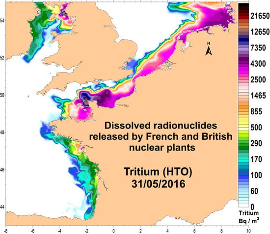
2.1. Dissolved Radionuclides as Oceanographic Tracers
- It must originate from one or a small number of clearly identified release points;
- The release conditions must be precisely known (time, fluxes);
- Labeling in seawater must be significant, in particular in relation to the pre-existing background level. Labeling concerns seawaters where a significant concentration of radionuclide could be measured.
- The tracer must be soluble and not fix onto living organisms or sediments over time (i.e., the stable element is conservative in seawater);
- It must be possible to measure the tracer after dilution in the sea over hours, weeks, months or years after its release.
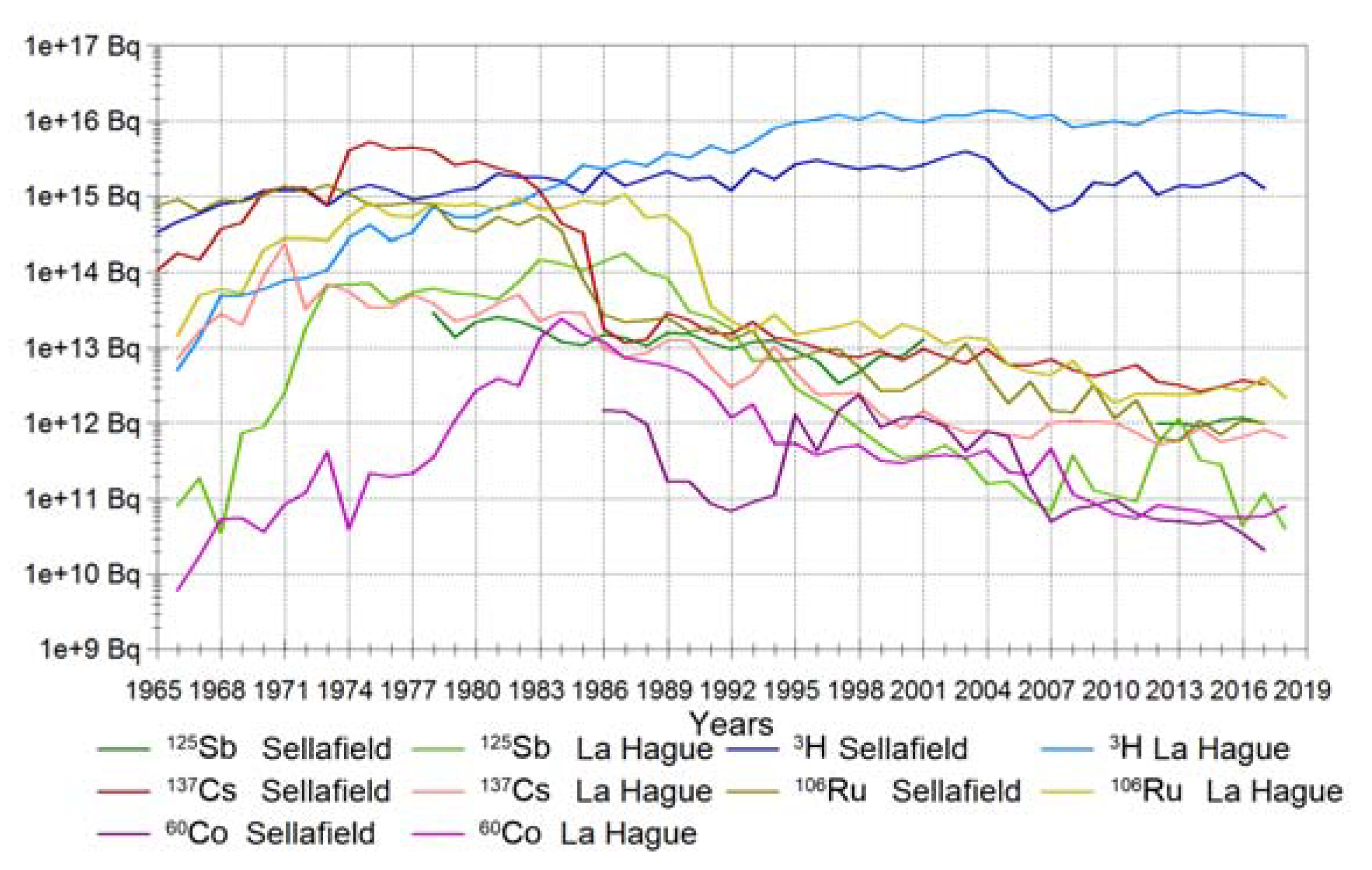
2.1.1. Gamma Emitters
2.1.2. Tritium
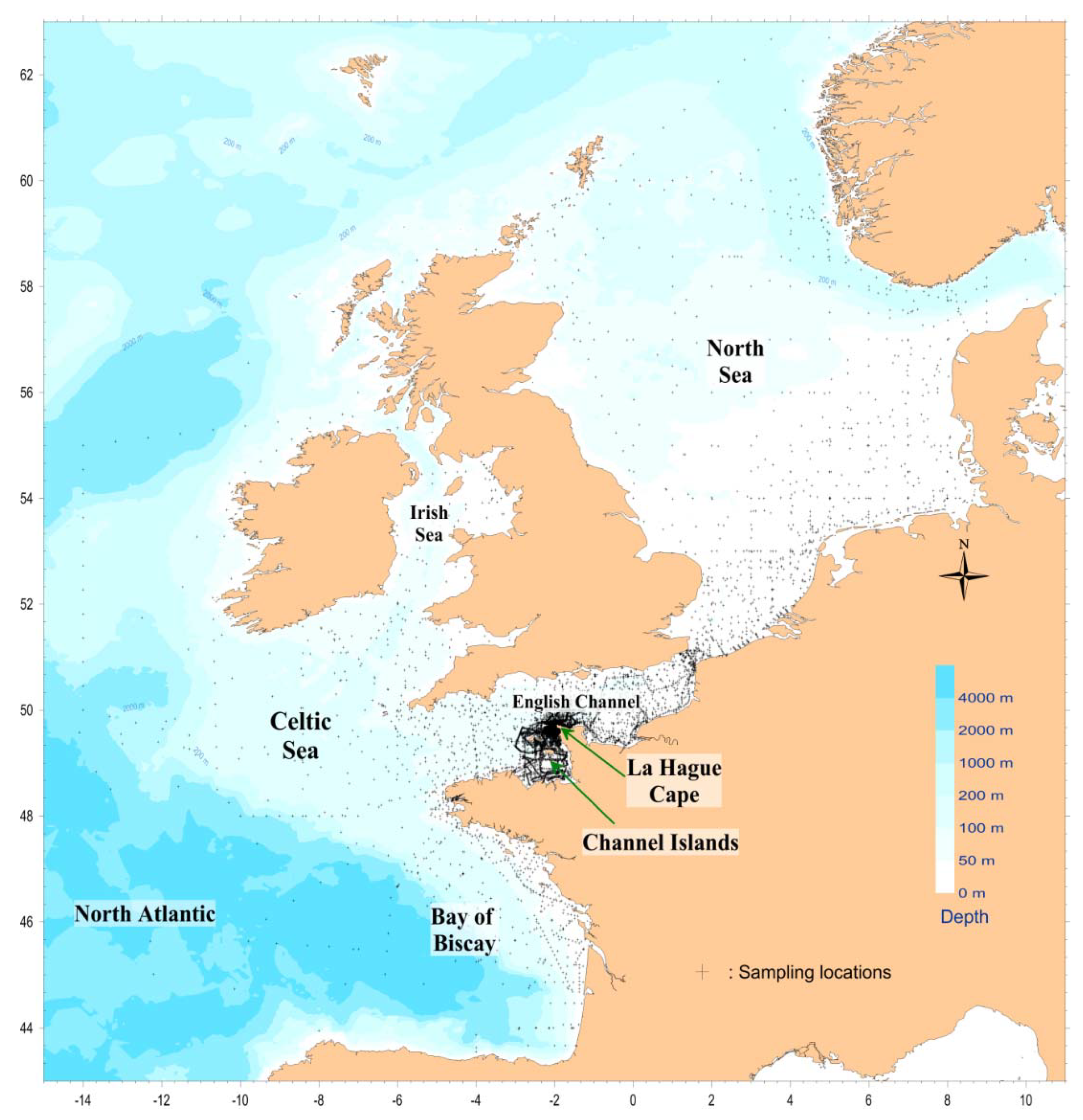
2.2. Database
2.2.1. Radionuclide Measurements in Seawater
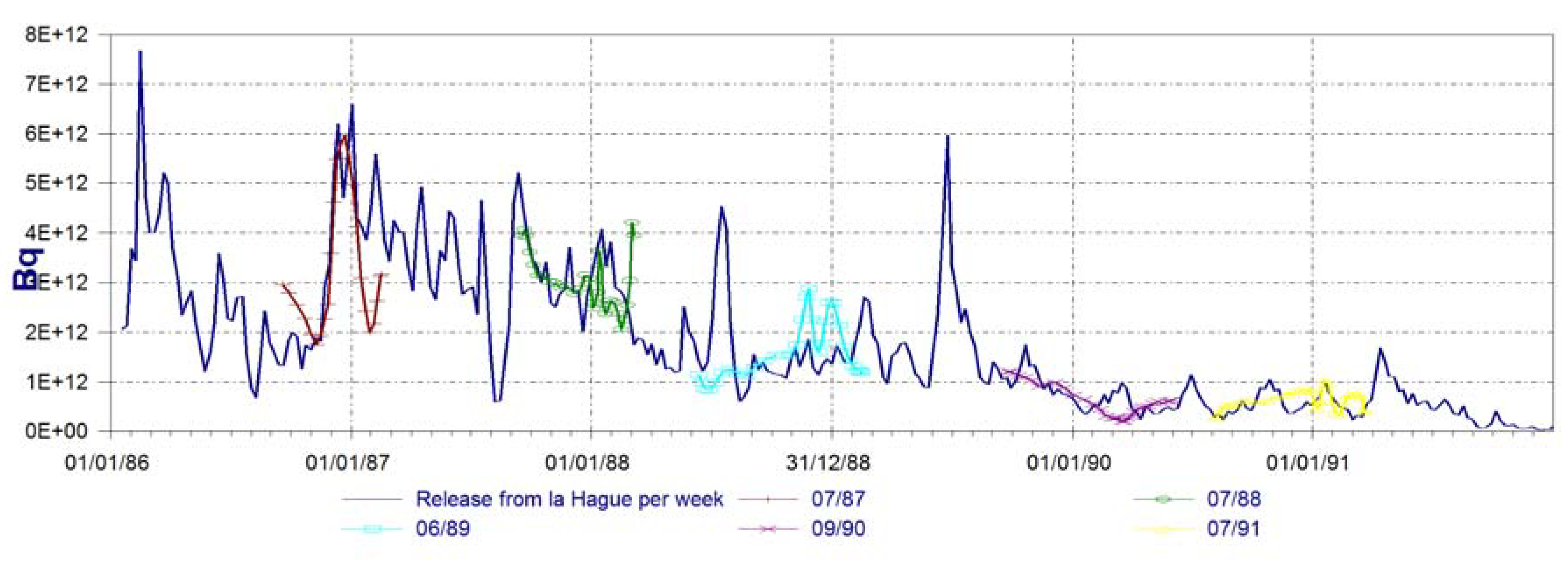
2.2.2. Radioactive Releases
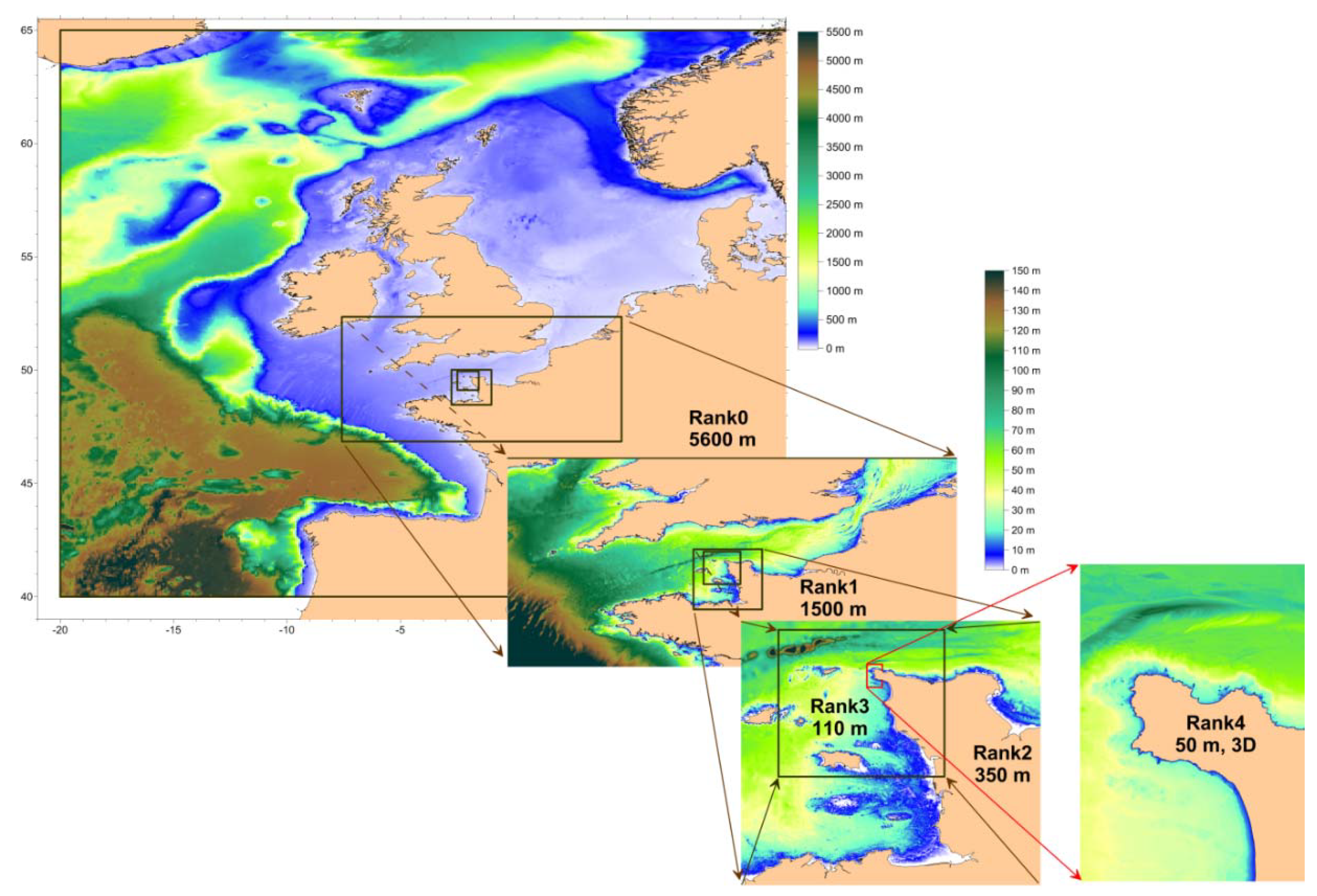
2.3. Hydrodynamic Models
2.3.1. 2D Modeling
2.3.2. 3D Modeling
2.3.3. 2D “Lagrangian Barycentric” Method
2.4. Sampling Close to An Outfall
2.4.1. Model Assisted Sampling
2.4.2. High Frequency In-Depth Sampling
- A sampling line designed to sample 10 depths simultaneously down to 65 m;
- A deep towed depressor (known as Dynalest), which maintains the line at depth close to the seabed;
- An automatic high-frequency sampler with volume, flux and depth control to get 1800 samples per hour.
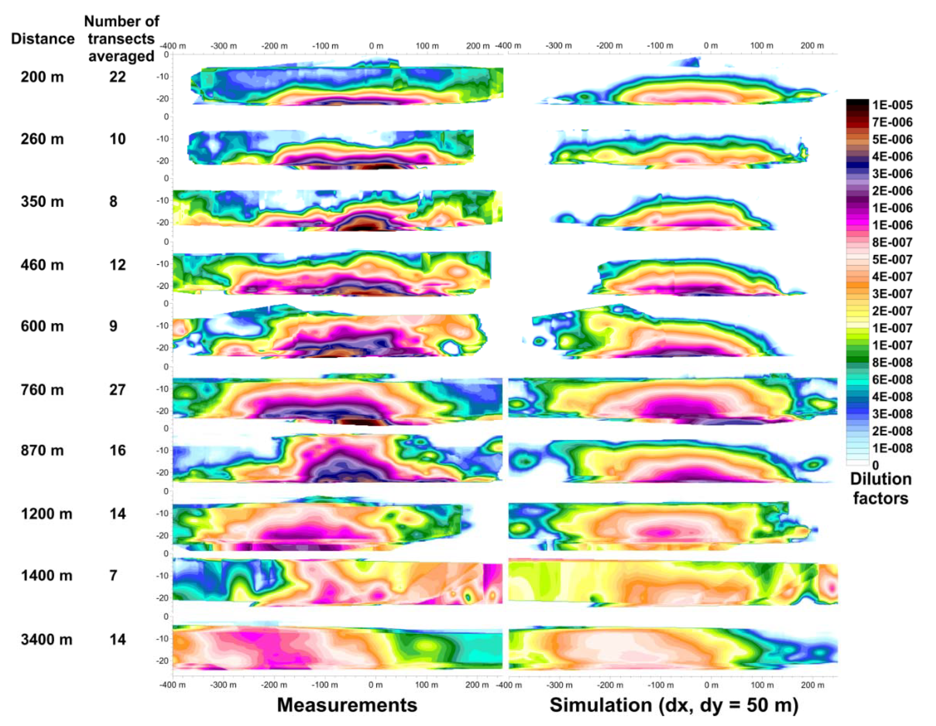
2.5. Methods for Model/Measurement Comparisons
2.5.1. Comparison with Individual Measurements
- : Measured tritium concentration of the n sample (Bq·m−3);
- : Mean measured tritium concentration (Bq·m−3);
- : Simulated tritium concentration of the n sample (Bq·m−3);
- : Mean simulated tritium concentration (Bq·m−3);
- Number of samples.
- Maximum concentration in the plume;
- Mean concentration in the plume;
- Width of plume intersected;
- Distance between maximal measured and simulated plume positions;
- Plume width discrepancy;
- Average and maximum concentration discrepancies;
- Dilution rate discrepancy.
- Bq·L−1M: measured concentrations
- Bq·L−1R: released flux
2.5.2. Radionuclides Inventories
2.6. Scales for Model/Measurement Comparisons
3. Applications
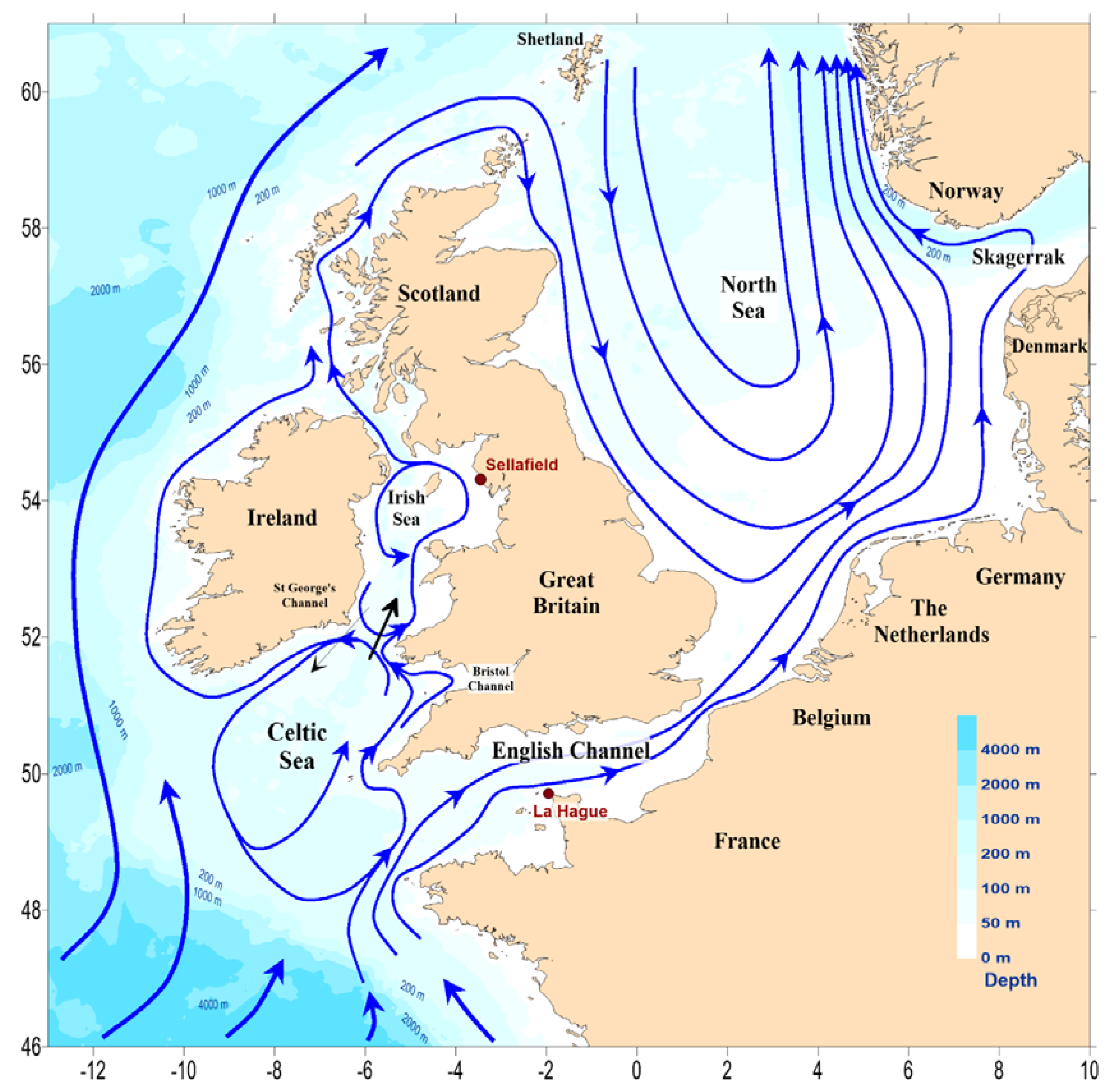
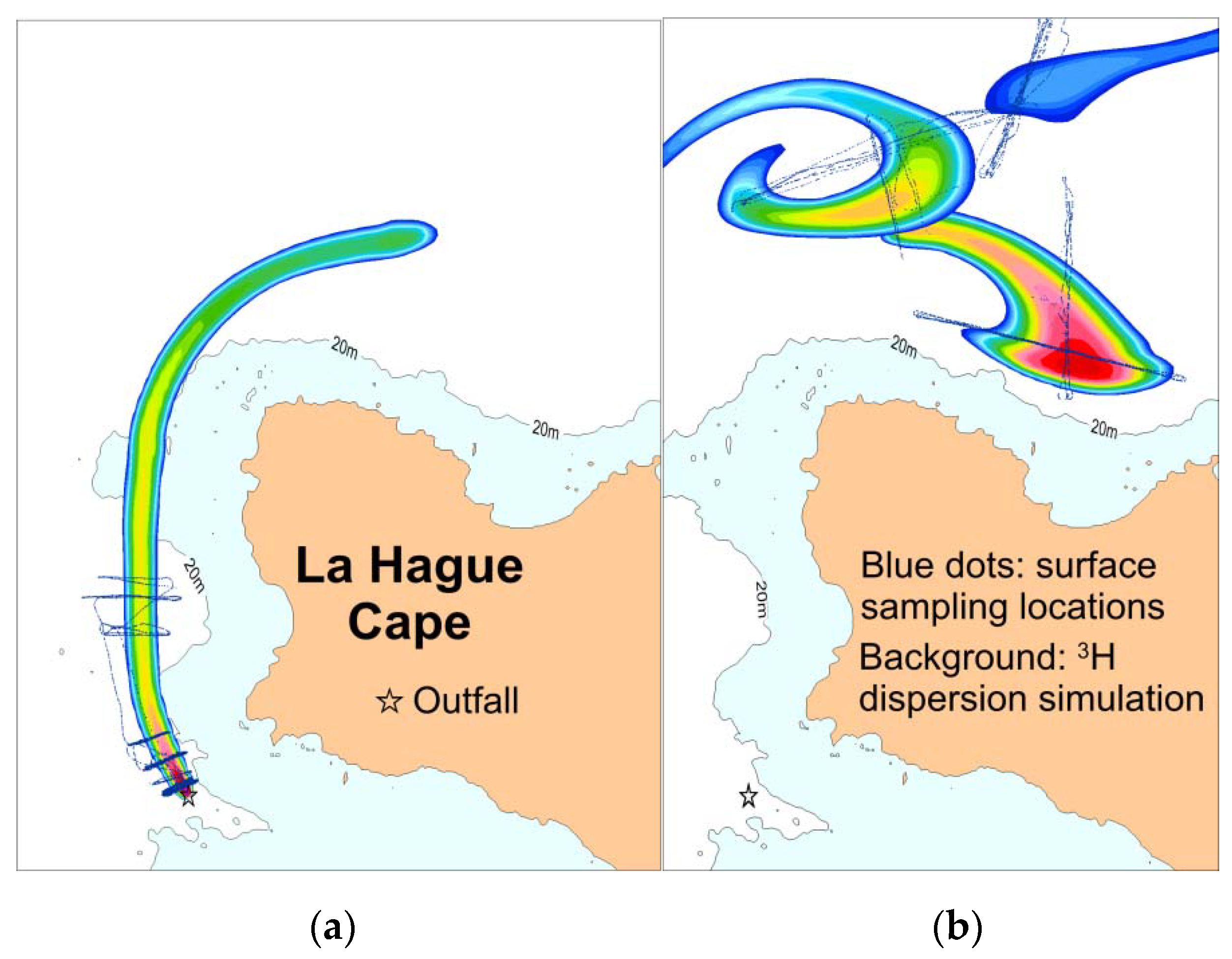
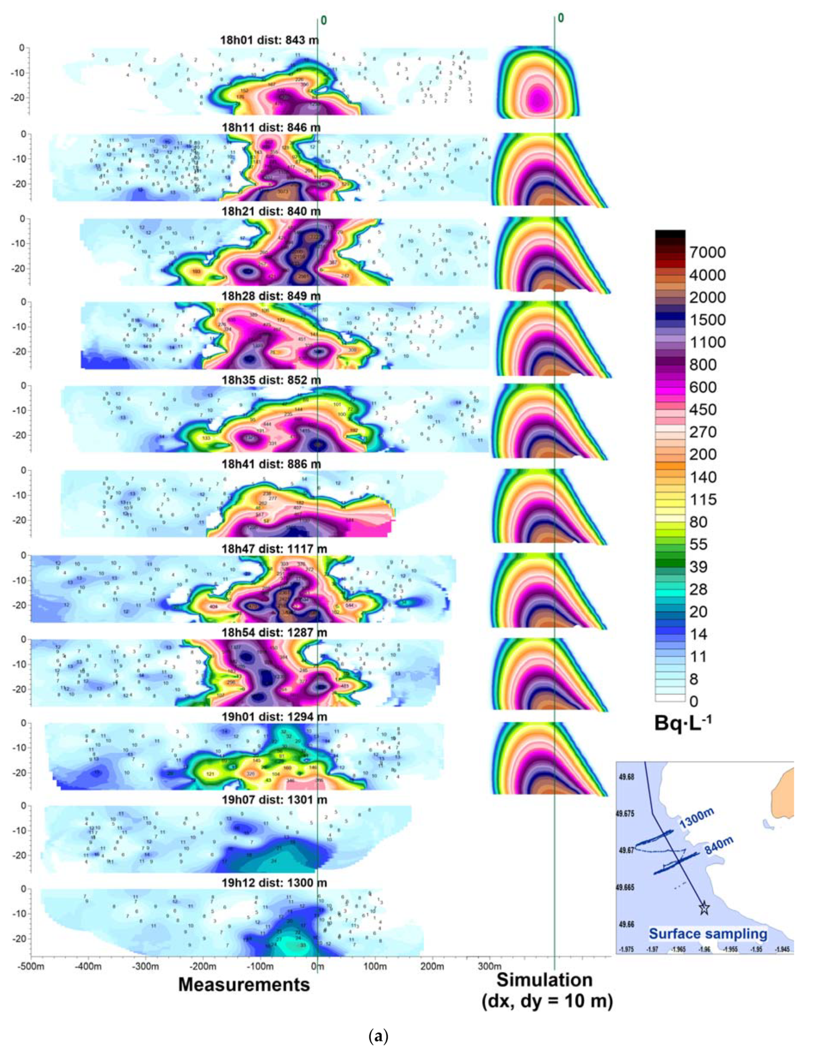
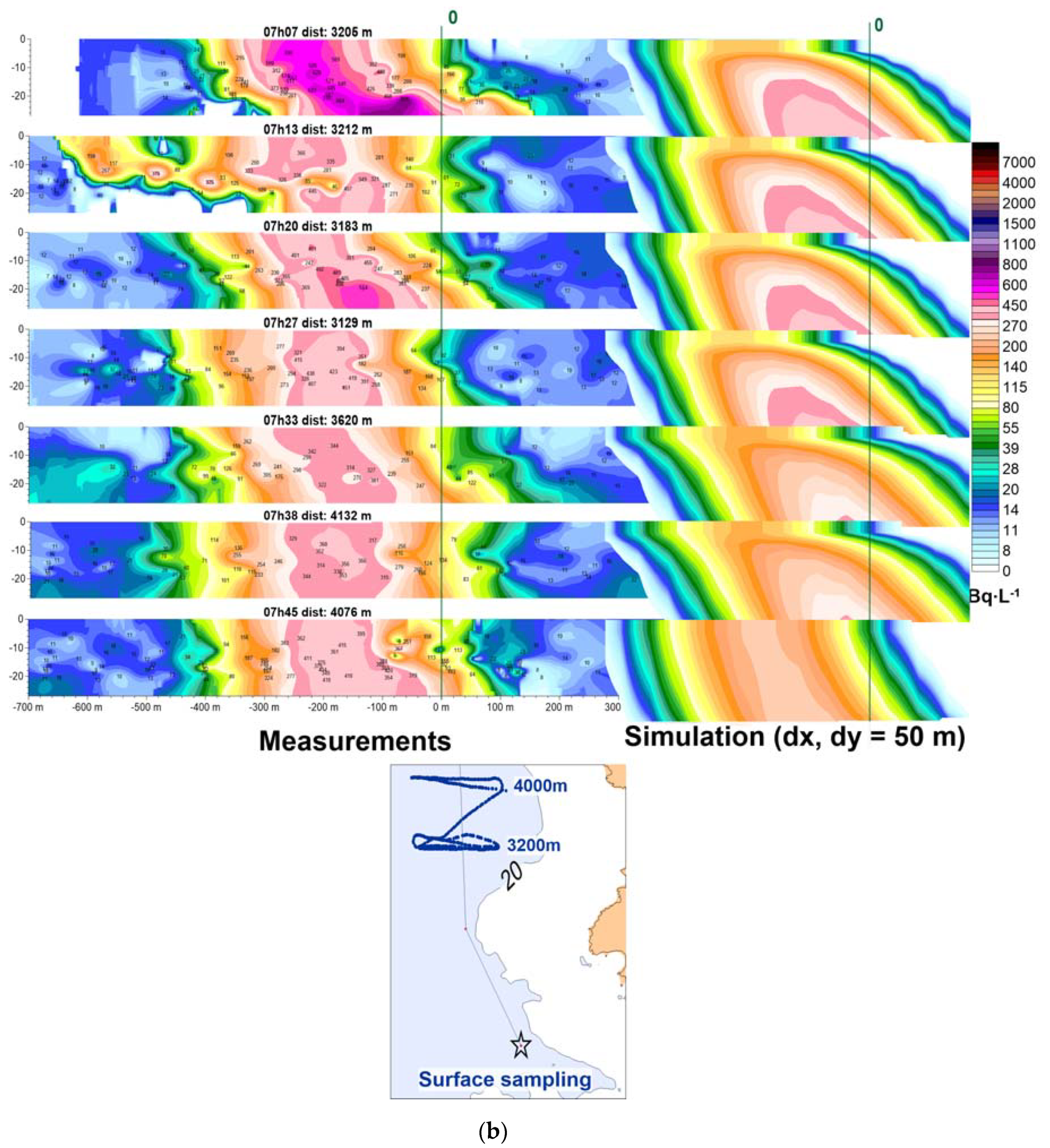
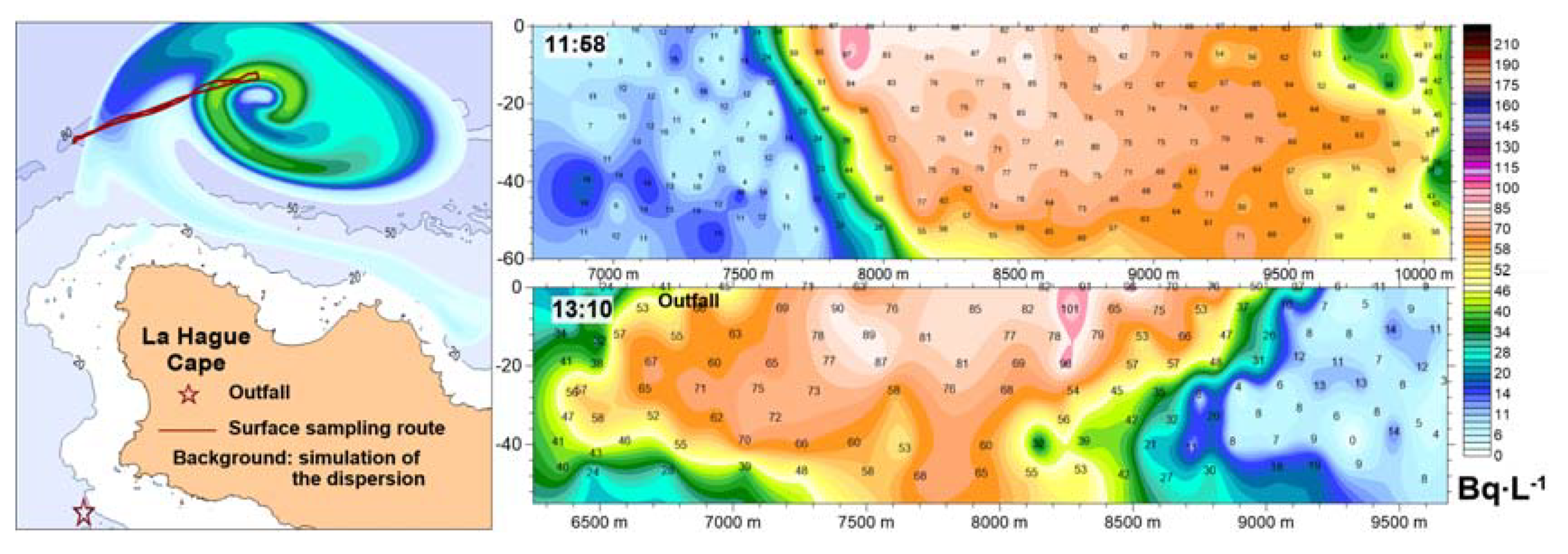
3.1. La Hague Cape, Short Scale/High Resolution Studies
3.1.1. The La Hague Cape Main Characteristics for Dissolved Radionuclide Dispersion
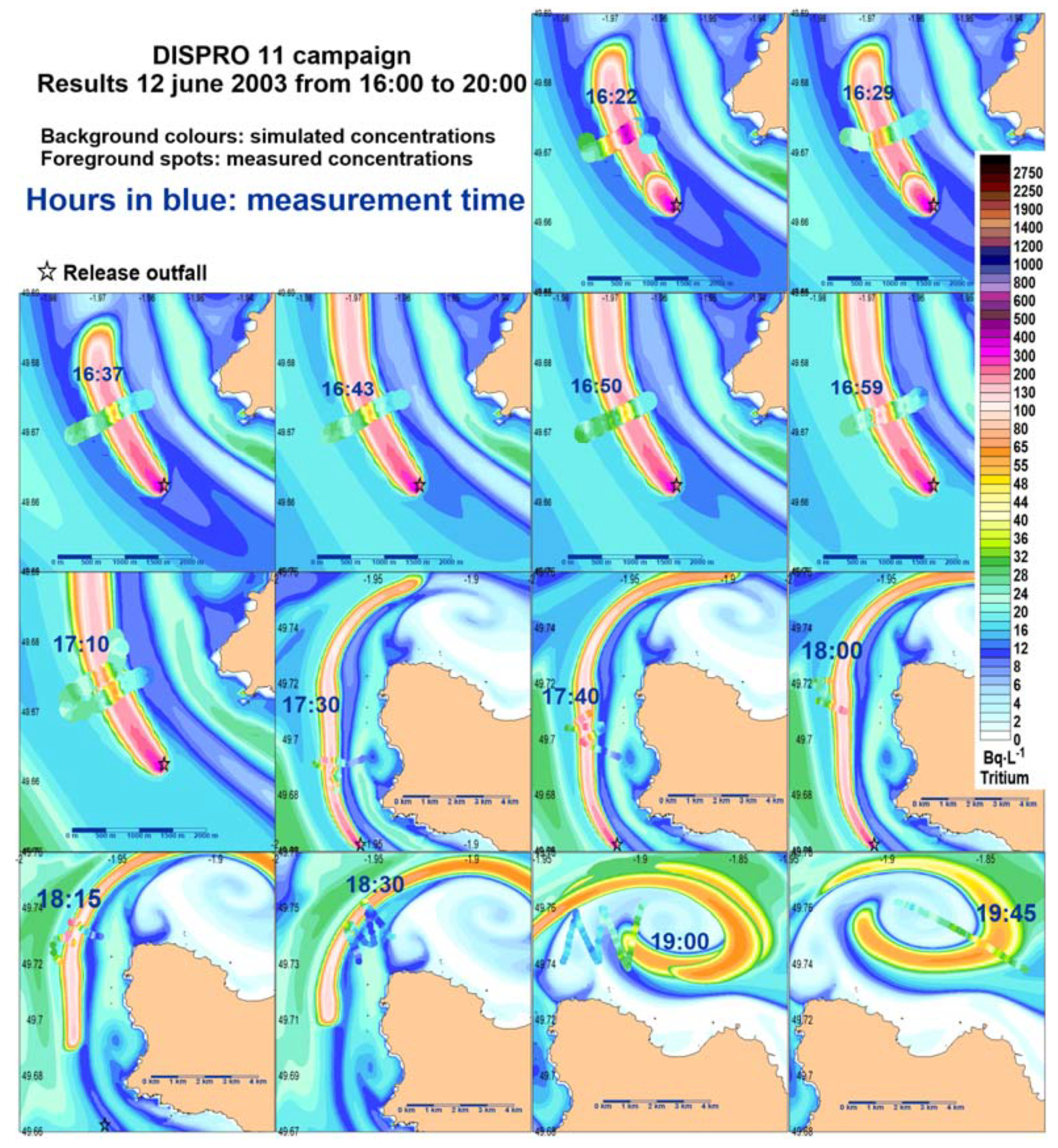
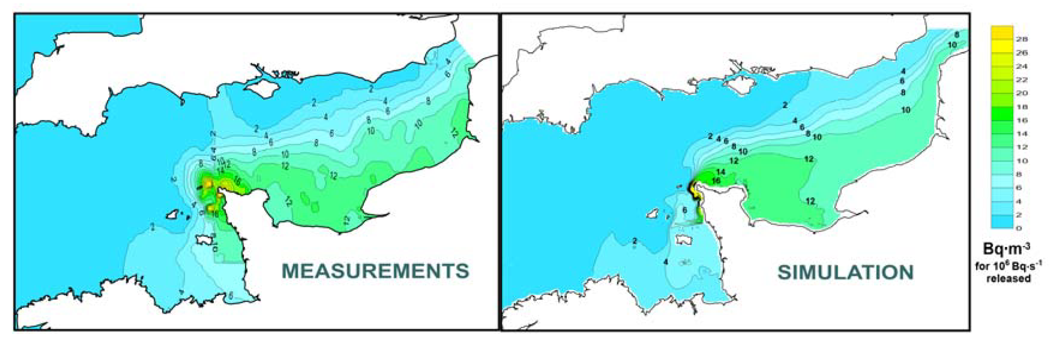
3.1.2. 3D Dispersion: Super Tidal Time Scale
3.1.3. 2D Dispersion: Tidal Time Scale
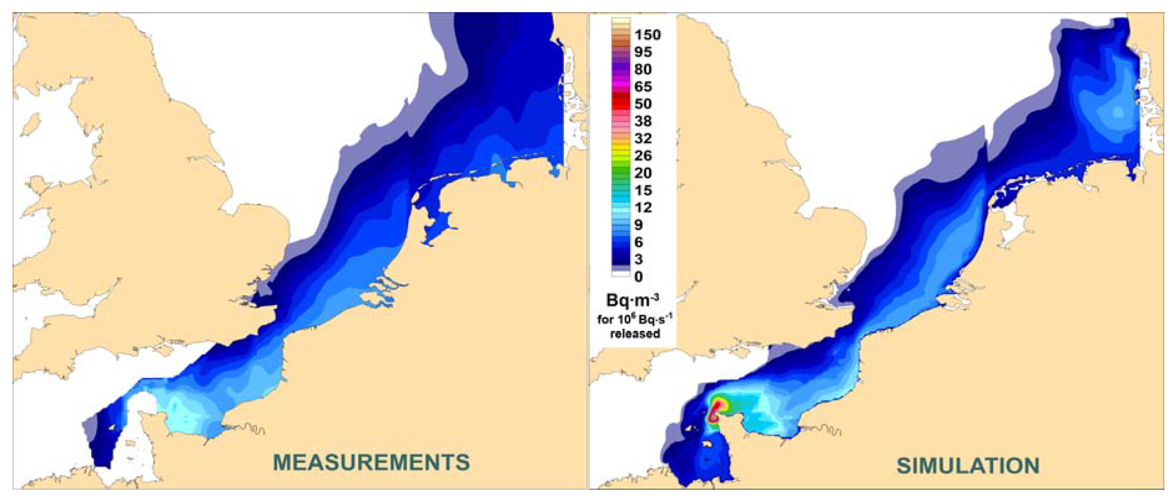
3.2. Large Scale Model/Measurement Comparisons: Multi Tidal Time Scales
3.2.1. Individual Measurements
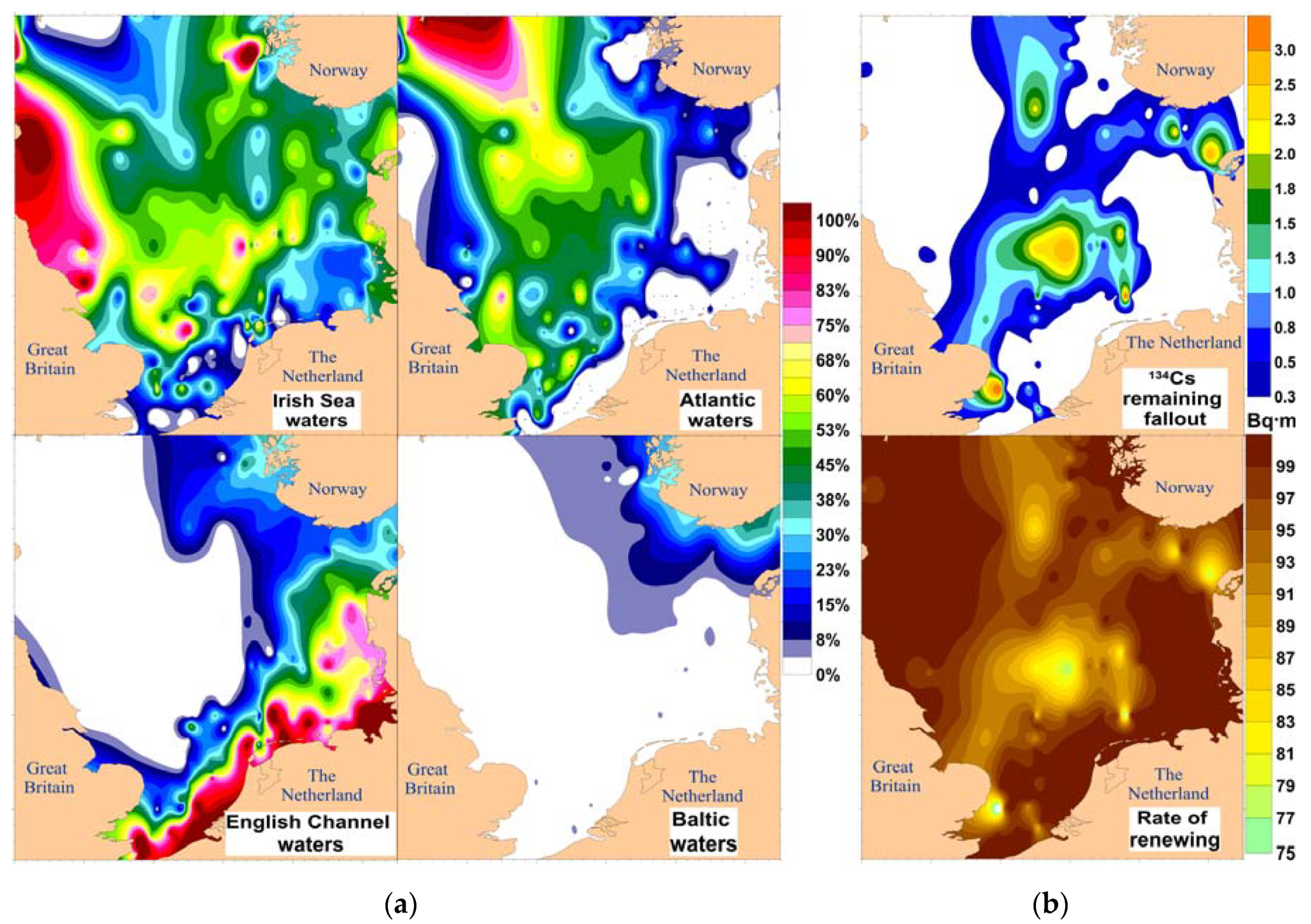
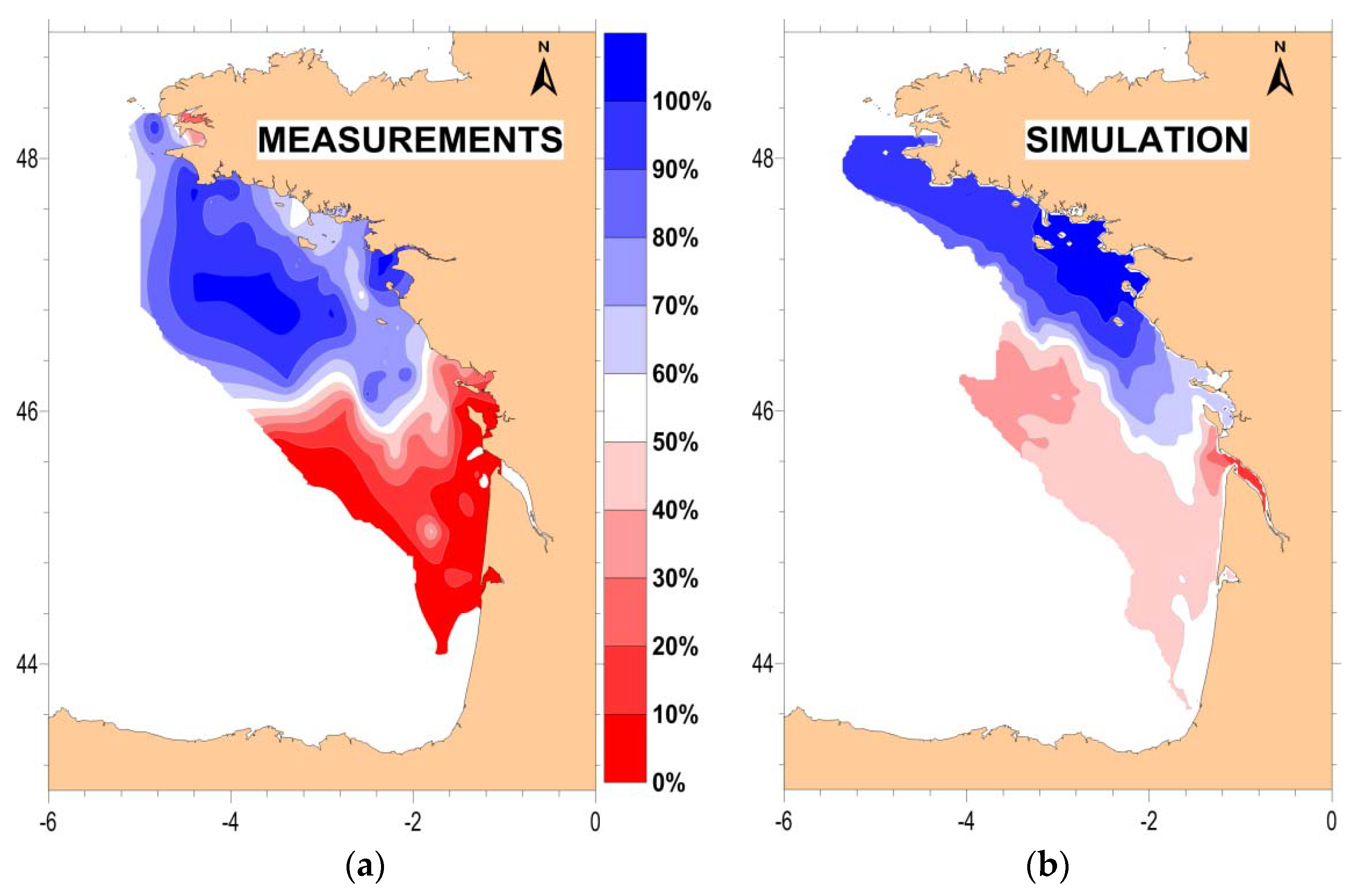
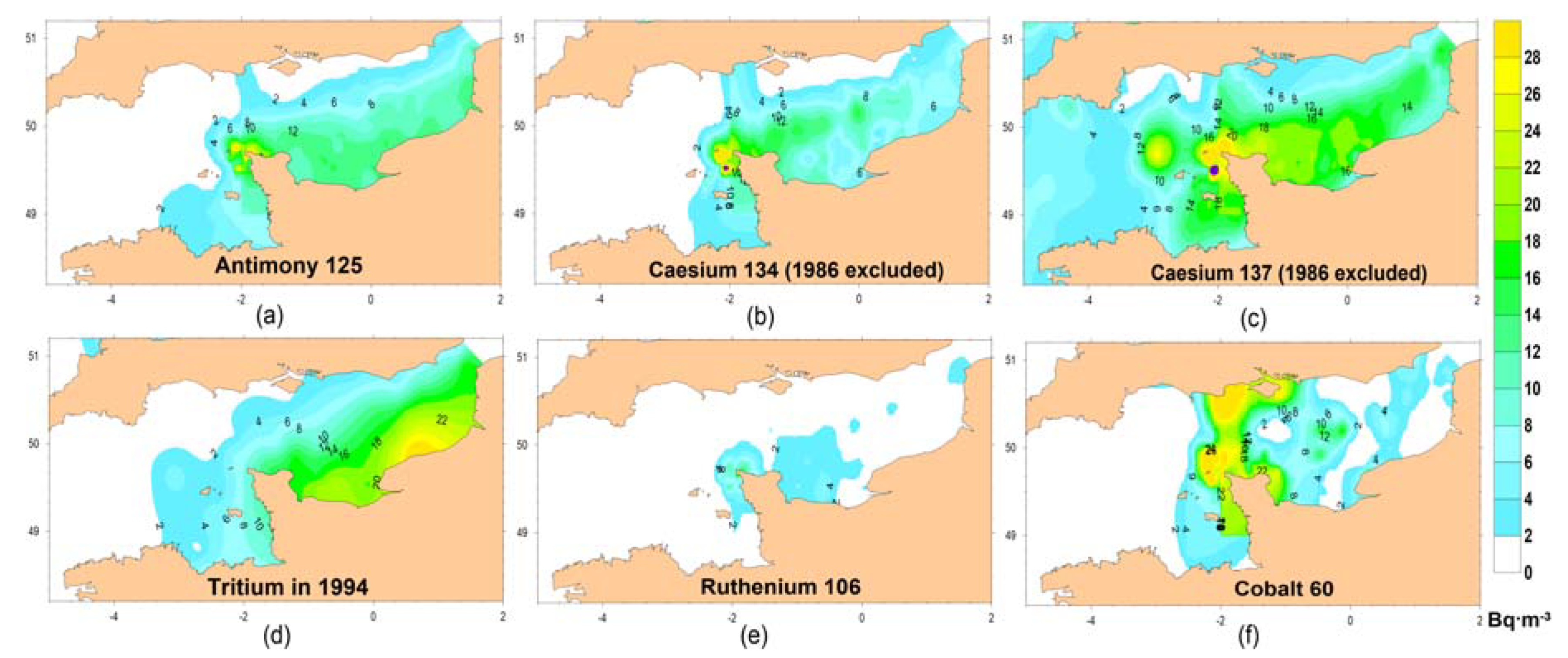
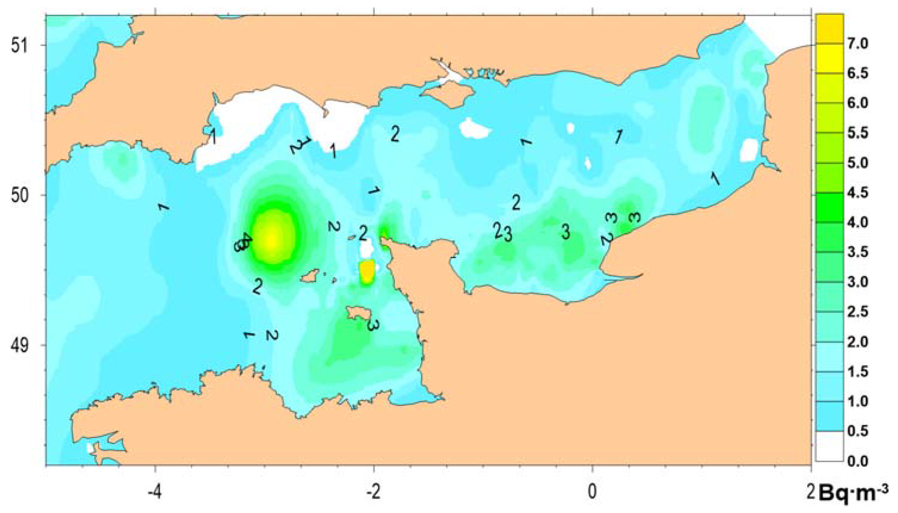
3.2.2. Water Masses Labeling
3.2.3. Integration of Normalized Contributions
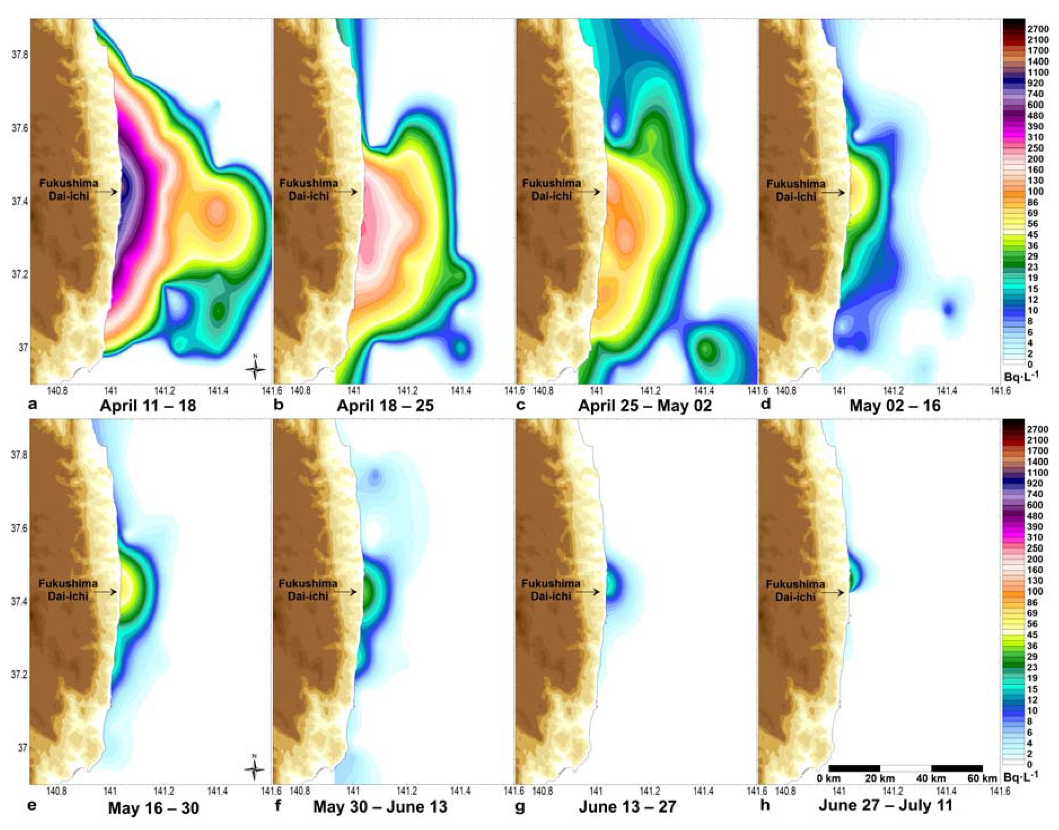
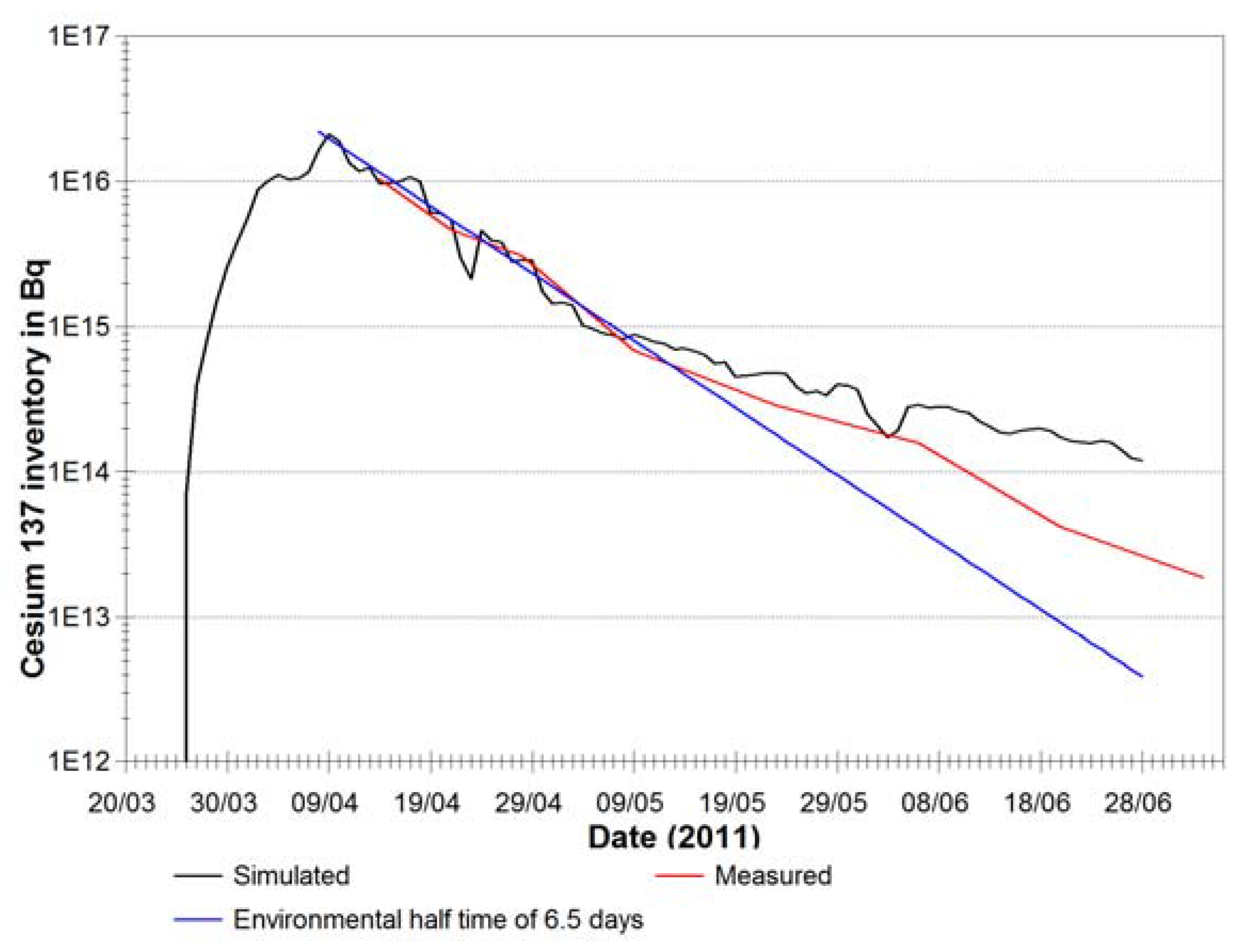
3.2.4. Inventories
4. Discussion
4.1. Radiotracers
4.2. Hydrodynamic Models
4.3. Scales for Model/Measurement Comparisons
4.4. Sampling Tools
4.5. Radionuclides Inventories
4.6. Normalization
4.7. Perspectives
Supplementary Materials
Author Contributions
Funding
Acknowledgments
Conflicts of Interest
Appendix A

| Campaign Name | Year | Area abr. | Stat. nb. | Lon. Min. | Lon. Max. | Lat. min. | Lat. max. | H3 | Cs137 | Cs134 | Sb125 | Ru106 | Co60 | ||||||
|---|---|---|---|---|---|---|---|---|---|---|---|---|---|---|---|---|---|---|---|
| Nb. | Max. meas. | Nb. | Max. meas. | Nb. | Max. meas. | Nb. | Max. meas. | Nb. | Max. meas. | Nb. | Max. meas. | ||||||||
| Cirolana0582 | 1982 | EC, CS, NS | 42 | −7.0 | 2.0 | 49.5 | 58.7 | 39 | 642 | ||||||||||
| Cirolana0583 | 1983 | EC, CS, IS | 54 | −7.5 | −1.9 | 49.3 | 54.7 | 44 | 13,283 | 22 | 688 | 14 | 459 | 36 | 7511 | 1 | 21.8 | ||
| Clione0983 | 1983 | EC, CS | 36 | −8.5 | 1.3 | 48.6 | 51.6 | 35 | 37.0 | ||||||||||
| GEA0983 | 1983 | EC, CI | 12 | −2.5 | −2.2 | 49.3 | 49.6 | 12 | 19.2 | 6 | 3.0 | 9 | 23.8 | 9 | 69 | ||||
| Thalassa1283 | 1983 | EC, BB | 56 | −4.8 | 0.3 | 47.4 | 50.0 | 55 | 59.2 | 31 | 10.0 | 45 | 149 | 44 | 207 | 8 | 44.4 | ||
| Pluteus0583 | 1983 | EC, CI, NS | 119 | −2.7 | 2.9 | 48.9 | 51.3 | 115 | 69.2 | 21 | 15.5 | 105 | 1668 | 79 | 3256 | ||||
| Pluteus0686 | 1986 | EC, CI | 185 | −4.8 | 2.0 | 48.3 | 51.3 | 184 | 34.5 | 141 | 6.7 | 163 | 211 | 134 | 686 | 29 | 13.0 | ||
| Ferry1986 | 1986 | EC, CS | 31 | −8.3 | −4.0 | 48.8 | 51.8 | 31 | 15.4 | 7 | 5.3 | ||||||||
| Pluteus1286 | 1986 | EC | 47 | −1.8 | −1.4 | 49.7 | 50.3 | 47 | 18.6 | 27 | 5.2 | 44 | 89.7 | 38 | 180 | 27 | 8.8 | ||
| GEA1986 | 1986 | EC, CS | 97 | −6.0 | 1.9 | 48.7 | 51.2 | 97 | 53.3 | 80 | 21.8 | 45 | 46.3 | 34 | 315 | 13 | 8.9 | ||
| Nies0187 | 1987 | NS | 29 | 1.5 | 9.2 | 51.0 | 55.0 | 29 | 84.0 | 23 | 13.0 | ||||||||
| Aurélia0387 | 1987 | NS | 31 | 3.0 | 4.7 | 51.7 | 53.0 | 31 | 15.5 | 31 | 5.7 | 30 | 57.1 | 29 | 213 | ||||
| Sépia1987 | 1987 | EC, NS | 14 | 1.3 | 2.3 | 50.3 | 51.2 | 14 | 11.2 | 4 | 1.8 | 14 | 48.5 | 14 | 121 | 1 | 0.4 | ||
| Manche0687 | 1987 | EC | 50 | −1.9 | 0.3 | 49.6 | 50.8 | 50 | 10.0 | 10 | 3.0 | 50 | 84.1 | 40 | 495 | 7 | 10.4 | ||
| Luctor0687 | 1987 | NS | 63 | 2.0 | 3.9 | 51.1 | 51.9 | 63 | 31.2 | 19 | 4.0 | 61 | 62.2 | 19 | 120 | ||||
| Pluteus0887 | 1987 | EC, CI, NS | 165 | −4.0 | 7.9 | 48.7 | 54.2 | 164 | 90.5 | 84 | 39.6 | 152 | 70.1 | 139 | 180 | 14 | 2.5 | ||
| Aurélia1187 | 1987 | NS | 6 | 3.5 | 4.6 | 52.1 | 52.7 | 6 | 12.8 | 4 | 1.6 | 4 | 57.4 | 6 | 104 | ||||
| GEA 1987 | 1987 | EC | 16 | −2.0 | 2.5 | 49.5 | 51.2 | 16 | 11.8 | 11 | 2.6 | 16 | 44.8 | 13 | 143 | 5 | 2.2 | ||
| Aurélia0488 | 1988 | NS | 9 | 3.5 | 4.6 | 52.1 | 52.9 | 9 | 12.6 | 6 | 58.0 | ||||||||
| Pluteus0488 | 1988 | EC | 44 | −1.7 | 1.6 | 49.5 | 51.1 | 44 | 11.1 | 1 | 1.1 | 43 | 43.6 | 28 | 116 | ||||
| Pluteus0688 | 1988 | EC | 105 | −5.1 | 1.6 | 49.4 | 51.1 | 104 | 12.2 | 81 | 112 | 63 | 222 | ||||||
| Pluteus0788 | 1988 | EC, CI | 103 | −4.0 | −1.1 | 48.6 | 49.8 | 103 | 12.5 | 4 | 1.4 | 94 | 464 | 42 | 324 | 6 | 2.7 | ||
| GEA0788 | 1988 | EC | 105 | −5.0 | 1.6 | 49.4 | 51.1 | 104 | 12.2 | 21 | 1.9 | 81 | 180 | 64 | 222 | 5 | 2.6 | ||
| Tramanor1 | 1988 | EC, NS | 256 | −2.0 | 9.0 | 49.7 | 60.2 | 242 | 70.7 | 192 | 13.3 | 186 | 48.9 | 107 | 189 | 2 | 2.0 | ||
| Gedynor | 1989 | EC, NS | 127 | −4.0 | 8.5 | 49.2 | 58.9 | 119 | 38.8 | 37 | 4.3 | 89 | 57.1 | 33 | 151 | 1 | 1.6 | ||
| RadeBrest0689 | 1989 | CI | 23 | −4.6 | −4.3 | 48.3 | 48.4 | 23 | 5.9 | ||||||||||
| RadeBrest0789 | 1989 | CI | 23 | −4.6 | −4.3 | 48.3 | 48.4 | 23 | 6.3 | ||||||||||
| GEA0989 | 1989 | EC, CI | 88 | −2.6 | −0.9 | 49.4 | 50.2 | 87 | 31.5 | 57 | 7.8 | 88 | 107.4 | 80 | 355 | 23 | 15.9 | ||
| Pluteus0989 | 1989 | EC, CI | 124 | −2.8 | −1.0 | 49.2 | 50.3 | 124 | 37.0 | 71 | 4.8 | 123 | 203.0 | 100 | 985 | 53 | 13.9 | ||
| RadeBrest0390 | 1990 | CI | 46 | −4.6 | −4.2 | 48.3 | 48.4 | 46 | 4.1 | ||||||||||
| Tramanor2 | 1990 | EC, CI, NS | 205 | −6.0 | 8.5 | 48.3 | 60.1 | 171 | 23.7 | 59 | 2.6 | 137 | 14.5 | 116 | 90 | 39 | 15.2 | ||
| FluxManche0990 | 1990 | EC | 32 | 1.2 | 1.6 | 50.7 | 51.1 | 24 | 14.8 | 9 | 57.0 | 26 | 23.1 | 17 | 56 | ||||
| Cirolana1 | 1991 | EC, NS | 55 | −1.7 | 4.5 | 49.8 | 55.2 | 44 | 21.9 | 11 | 1.1 | 35 | 13.8 | 33 | 67 | 24 | 2.7 | ||
| Tramanor3 | 1991 | EC, NS | 162 | −1.8 | 9.1 | 49.4 | 63.3 | 144 | 28.0 | 65 | 1.7 | 116 | 18.9 | 73 | 37 | 41 | 1.4 | ||
| Cirolana2 | 1992 | EC, NS | 42 | −1.1 | 5.6 | 49.7 | 55.2 | 38 | 18.5 | 3 | 0.5 | 29 | 11.4 | 18 | 8 | 11 | 3.3 | ||
| GolfeNormandBreton0492 | 1992 | EC, CI | 39 | −3.0 | −1.7 | 48.7 | 49.8 | 37 | 7.5 | 24 | 0.5 | 37 | 21.0 | 7 | 14 | 15 | 2.4 | ||
| Valdivia1993 | 1993 | EC, CS, IS, NS | 63 | −6.0 | 11.0 | 49.8 | 58.5 | 62 | 259 | 60 | 2.1 | 60 | 13.8 | 58 | 10 | 56 | 3.9 | ||
| Arrho1994 | 1994 | MS | 9 | 4.7 | 4.9 | 43.3 | 43.4 | 9 | 5.1 | 5 | 1.1 | 5 | 3.6 | 7 | 68 | 5 | 0.4 | ||
| Gedymac1994 | 1994 | EC, CI, CS, IS | 222 | −8.4 | 1.5 | 48.0 | 54.5 | 95 | 8870 | 211 | 222 | 55 | 1.4 | 95 | 30.8 | 33 | 9 | 43 | 2.5 |
| Dymanche1994 | 1994 | EC | 81 | −1.9 | 1.5 | 49.3 | 51.1 | 81 | 27.7 | 45 | 2.4 | 47 | 5.8 | 6 | 13 | 18 | 1.3 | ||
| RadialeCh-Wh0295 | 1995 | EC | 8 | −1.7 | −1.0 | 49.7 | 50.7 | 4 | 5860 | 8 | 5.6 | 1 | 2.4 | 2 | 5 | 5 | 0.9 | ||
| RadialeCh-Wh0395 | 1995 | EC | 7 | −1.7 | −1.0 | 49.7 | 50.7 | 6 | 4.4 | 1 | 1.5 | 2 | 0.5 | ||||||
| RadialeCh-Wh0595 | 1995 | EC | 8 | −1.7 | −1.0 | 49.7 | 50.7 | 8 | 4.7 | 1 | 0.3 | 3 | 1.3 | 1 | 4 | 3 | 0.5 | ||
| Omex 0695 | 1995 | CI, NA | 7 | −13.7 | −6.6 | 47.4 | 56.6 | 7 | 1.7 | ||||||||||
| Omex 0895 | 1995 | CI, NA | 8 | −14.1 | −7.4 | 47.7 | 50.6 | 8 | 3.3 | ||||||||||
| RadialeCh-Wh0795 | 1995 | EC, CI | 31 | −2.7 | −1.0 | 49.3 | 50.6 | 31 | 9.0 | 25 | 0.7 | 28 | 1.6 | 21 | 2 | 25 | 0.9 | ||
| RadialeCh-Wh0995 | 1995 | EC | 8 | −1.9 | −1.1 | 49.7 | 50.6 | 8 | 7.2 | 4 | 0.3 | 5 | 3.6 | 4 | 10 | 8 | 0.6 | ||
| RadialeCh-Wh1195 | 1995 | EC, CI | 37 | −2.6 | −1.6 | 49.0 | 49.9 | 37 | 5.8 | 21 | 0.2 | 35 | 2.0 | 33 | 34 | 28 | 0.7 | ||
| Ferry0396 | 1996 | EC, CS | 23 | −8.3 | −4.0 | 48.7 | 51.8 | 4 | 719 | 23 | 2.7 | 3 | 0.7 | ||||||
| FondDeBaie0496 | 1996 | EC | 15 | −2.3 | −1.6 | 48.6 | 48.8 | 5 | 3710 | 14 | 3.4 | 1 | 0.1 | 13 | 0.7 | 3 | 1 | 9 | 0.6 |
| Ferry0696 | 1996 | EC | 8 | −1.9 | −1.7 | 49.7 | 50.7 | 8 | 5.1 | 2 | 0.5 | 5 | 2.8 | 4 | 3 | 6 | 0.5 | ||
| FondDeBaie0796 | 1996 | EC | 10 | −2.4 | −2.0 | 48.6 | 48.7 | 10 | 3200 | 10 | 3.3 | 7 | 0.7 | 4 | 0.4 | ||||
| Irma1996 | 1996 | EC | 83 | −6.0 | −1.3 | 48.1 | 50.5 | 60 | 21,000 | 71 | 6.1 | 1 | 0.3 | 9 | 2.1 | 10 | 11 | 19 | 6.1 |
| Arcane1997 | 1997 | CS, NA | 52 | −12.8 | −3.3 | 39.1 | 45.6 | 22 | 268 | 43 | 2.5 | ||||||||
| Ferry1997 | 1997 | EC | 19 | −4.2 | −1.6 | 48.8 | 50.7 | 11 | 484 | 19 | 4.2 | 1 | 0.9 | ||||||
| FluxSed1998 | 1998 | EC, CI | 66 | −6.3 | 0.1 | 48.6 | 50.2 | 66 | 5.9 | 5 | 1.9 | 9 | 13 | 8 | 1.0 | ||||
| Atmara1998 | 1998 | EC, CS, NA | 196 | −14.0 | −3.6 | 45.5 | 55.7 | 130 | 1930 | 191 | 16.1 | ||||||||
| Cirolana2000 | 2000 | CS, BB | 35 | −11.5 | 1.5 | 47.3 | 52.3 | 35 | 1323 | ||||||||||
| Ovide2002 | 2002 | NA | 60 | −42.6 | −6.2 | 35.8 | 59.8 | 45 | 377 | 15 | 2.7 | ||||||||
| Dispro08 | 2002 | LH, EC, CI | 1029 | −2.4 | 0.9 | 49.4 | 50.0 | 845 | 45,103 | ||||||||||
| Dispro09 | 2002 | LH, EC, CI | 1058 | −2.4 | −1.6 | 49.5 | 49.8 | 1046 | 2,355,208 | ||||||||||
| Dispro10 | 2002 | LH, EC, CI | 1899 | −2.2 | −1.6 | 49.6 | 49.8 | 1890 | 3,604,897 | ||||||||||
| Dispro11 | 2003 | LH, EC, CI | 2398 | −2.1 | −1.7 | 49.5 | 49.8 | 2397 | 15,32,137 | ||||||||||
| Dispro12 | 2003 | LH, EC, CI | 640 | −2.9 | −1.7 | 48.7 | 49.9 | 587 | 12,111 | ||||||||||
| Ovide2004 | 2004 | NA | 31 | −42.9 | −9.8 | 40.3 | 59.9 | 17 | 236 | 14 | 2.4 | ||||||||
| Dispro2004 | 2004 | LH, EC, CI | 3539 | −2.9 | −1.2 | 48.6 | 50.0 | 3537 | 392,028 | ||||||||||
| Dispro2005 | 2005 | LH, EC, CI | 4143 | −2.4 | 1.5 | 49.3 | 50.7 | 4103 | 268,816 | ||||||||||
| Disver2008 | 2008 | LH, EC, CI | 796 | −2.0 | −2.0 | 49.7 | 49.7 | 784 | 190,660 | ||||||||||
| Aspex2009 | 2009 | BB | 36 | −6.0 | −1.5 | 44.0 | 47.8 | 34 | 336 | ||||||||||
| Ovide2010 | 2010 | NA | 1 | −19.1 | −19.1 | 45.8 | 45.8 | 1 | 76 | ||||||||||
| Aspex2010 | 2010 | BB | 62 | −6.4 | −1.6 | 44.0 | 48.3 | 62 | 266 | ||||||||||
| Disver2010 | 2010 | LH | 5556 | −2.0 | −2.0 | 49.7 | 49.7 | 5314 | 7,029,776 | ||||||||||
| Disver2011 | 2011 | LH | 12498 | −2.0 | −1.9 | 49.7 | 49.8 | 12498 | 8,739,130 | ||||||||||
| Aspex2011 | 2011 | BB | 74 | −6.0 | −1.5 | 44.0 | 47.8 | 62 | 211 | ||||||||||
| Trimadu2013 | 2013 | NA | 18 | −13.2 | 55.5 | −32.4 | 34.9 | 17 | 80 | 12 | 1.1 | ||||||||
| Traces2014 | 2014 | EC, CI | 1205 | −3.0 | −1.6 | 48.6 | 49.8 | 1170 | 125,159 | ||||||||||
| Traces2015 | 2015 | EC, CI | 547 | −3.0 | −1.7 | 48.8 | 49.8 | 546 | 38,320 | ||||||||||
| Dynsedim2016 | 2016 | BB | 31 | −5.3 | −2.6 | 45.6 | 47.9 | 30 | 640 | ||||||||||
| Pelgas2016 | 2016 | BB | 130 | −5.8 | −1.3 | 43.7 | 47.9 | 125 | 583 | ||||||||||
| Plume2016 | 2016 | BB | 254 | −5.2 | −1.1 | 44.7 | 48.6 | 177 | 19,072 | 12 | 1.3 | ||||||||
| Goury (time series) | 1984–2018 | LH, EC | 744 | −1.9 | −1.9 | 49.7 | 49.7 | 266 | 41,999 | 615 | 79.9 | 260 | 62.3 | 498 | 223.1 | 484 | 1745 | 398 | 50.7 |
| Nb. total (campaigns): | 39,642 | 35,663 | 3492 | 1295 | 2242 | 1606 | 568 | ||||||||||||
| Nb. Total (all): | 80 | 40,386 | 35,929 | 4107 | 1555 | 2740 | 2090 | 966 | |||||||||||
References
- Guary, J.C.; Guéguéniat, P.; Pentreath, J. Radionucléides: A Tool for Oceanography; Elsevier Applied Science: Amsterdam, The Netherlands, 1988; p. 461. [Google Scholar]
- Kershaw, J.P.; Woodhead, D.S. Radionuclides in the Study of Marine Processes; Elsevier Applied Science: Amsterdam, The Netherlands, 1991; p. 393. [Google Scholar]
- Germain, P.; Guary, J.C.; Guéguéniat, P.; Métivier, H.E. Radionuclides in the Oceans. In Proceedings of the RADOC 96–97, Part 1, Inventories, Behaviour and Processes, Cherbourg-Octeville, France, 7–11 October 1996; Radioprotection Numéro Spécial, Colloques Volume 32, C2. Les Editions de Physique: Les Ulis, France, 1997; p. 422. [Google Scholar]
- Herrmann, J.; Kershaw, P.; Bailly du Bois, P.; Guéguéniat, P. The distribution of artificial radionuclides in the English Channel, southern North Sea, Skagerrak and Kattegat, 1990–1993. J. Mar. Syst. 1995, 6, 427–456. [Google Scholar] [CrossRef]
- Povinec, P.P.; Bailly du Bois, P.; Kershaw, P.; Nies, H.; Scotto, P. Temporal and spatial trends in the distribution of 137Cs in surface waters of Northern European Seas—A record of 40 years of investigations. Deep. Sea Res. Part II Top. Stud. Oceanogr. 2003, 50, 2785–2801. [Google Scholar] [CrossRef]
- Kershaw, P.; McCubbin, D.; Leonard, K. Continuing contamination of north Atlantic and Arctic waters by sellafield radionuclides. Sci. Total Environ. 1999, 237, 1119–1132. [Google Scholar]
- Kautsky, H. Investigations on the distribution of137Cs,134Cs and90Sr and the water mass transport times in the Northern North Atlantic and the North Sea. Ocean Dyn. 1987, 40, 49–69. [Google Scholar]
- Dahlgaard, H. Transfer of European coastal pollution to the arctic: Radioactive tracers. Mar. Pollut. Bull. 1995, 31, 33–37. [Google Scholar]
- Mitchell, P.I.; Holm, E.; Dahlgaard, H.; Boust, D.; Leonard, K.S.; Papucci, C.; Salbu, B.; Christensen, G.; Strand, P.; Sánchez-Cabeza, J.A.; et al. Radioecological Assessment of the Consequences of Contamination of Arctic Waters: Modelling the Key Processes Controlling Radionuclide Behaviour under Extreme Conditions (ARMARA); EC Nuclear Fission Safety Programme 1995-99 Contract No. F14P-CT95-0035 Final Report; Department of Experimental Physics University College Dublin: Dublin, Ireland, 1999; p. 151. [Google Scholar]
- Nies, H.; Albrecht, H.; Herrmann, J. Radionuclides in Water and Suspended Particulate Matter from the North Sea, Proceedings of the Radionuclides in the Study of Marine Processes, Norwich, UK, 10–13 September 1991; Kershaw, J.P., Woodhead, D.S., Eds.; Elsevier Applied Science: Amsterdam, The Netherlands, 1991; pp. 24–36. [Google Scholar]
- Bailly du Bois, P.; Germain, P.; Rozet, M.; Solier, L. Water Masses Circulation and Residence Time in the Celtic Sea and English Channel Approaches, Characterisation Based on Radionuclides Labelling from Industrial Releases, Proceedings of the International Conference on Radioactivity in Environment, Monaco, Principality of Monaco, 1–5 September 2002; Borretzen, P., Jolle, T., Strand, P., Eds.; Norwegian Radiation Protection Authority: Østerås, Norway, 2002; pp. 395–399. [Google Scholar]
- Guéguéniat, P.; Salomon, J.; Wartel, M.; Cabioch, L.; Fraizier, A. Transfer pathways and transit time of dissolved matter in the eastern English channel indicated by Space-Time radiotracers measurement and hydrodynamic modelling. Estuarine Coast. Shelf Sci. 1993, 36, 477–494. [Google Scholar] [CrossRef]
- Guéguéniat, P.; Bailly du Bois, P.; Gandon, R.; Salomon, J.; Baron, Y.; Leon, R. Spatial and temporal distribution (1987–1991) of 125Sb used to trace pathways and transit times of waters entering the north sea from the English channel. Estuarine Coast. Shelf Sci. 1994, 39, 59–74. [Google Scholar] [CrossRef]
- Guéguéniat, P.; Herrmann, J.; Kershaw, P.; Bailly du Bois, P.; Baron, Y. Artificial radioactivity in the English Channel and the North Sea. In Radionuclides in the Oceans, Inputs and Inventories, RADOC 96–97; Guéguéniat, P., Germain, P., Métivier, H., Eds.; Les Editions de Physique: Les Ulis, France, 1997; pp. 121–154. [Google Scholar]
- Guéguéniat, P.; Kershaw, P.; Hermann, J.; Bailly du Bois, P. New estimation of La Hague contribution to the artificial radioactivity of Norwegian waters (1992–1995) and Barents Sea (1992–1997). Sci. Total Environ. 1997, 202, 249–266. [Google Scholar] [CrossRef]
- Bailly du Bois, P.; Guéguéniat, P.; Gandon, R.; Leon, R.; Baron, Y. Percentage contribution of inputs from the Atlantic, Irish sea, English channel and baltic into the north sea during 1988: A Tracer-Based evaluation using artificial radionuclides. Neth. J. Sea Res. 1993, 31, 1–17. [Google Scholar] [CrossRef]
- Bailly du Bois, P.; Salomon, J.; Gandon, R.; Guéguéniat, P. A quantitative estimate of English channel water fluxes into the north sea from 1987 to 1992 based on radiotracer distribution. J. Mar. Syst. 1995, 6, 457–481. [Google Scholar] [CrossRef]
- Bailly du Bois, P.; Rozet, M.; Thoral, K.; Salomon, J.C. Improving Knowledge of Water-Mass Circulation in the English Channel Using Radioactive Tracers, Proceedings of the Radioprotection-Colloques, April 1997, Numéro spécial “Radionuclides in the Oceans”, RADOC 96–97, Proceedings Part 1 “Inventories, Behaviour and Processes”, Cherbourg-Octeville, France, 7–11 October 1996; Germain, P., Guary, J.C., Guéguéniat, P., Métivier, H., Eds.; Les Editions de Physique: Les Ulis, France, 1997; Volume 32, pp. 63–69. [Google Scholar]
- Bailly du Bois, P.; Guéguéniat, P. Quantitative assessment of dissolved radiotracers in the English channel: Sources, average impact of la Hague reprocessing plant and conservative behaviour (1983, 1986, 1988, 1994). Cont. Shelf Res. 1999, 19, 1977–2002. [Google Scholar] [CrossRef][Green Version]
- Guéguéniat, P.; Bailly du Bois, P.; Salomon, J.; Masson, M.; Cabioch, L. Fluxmanche radiotracers measurements: A contribution to the dynamics of the English channel and north sea. J. Mar. Syst. 1995, 6, 483–494. [Google Scholar] [CrossRef]
- Salomon, J.C.; Guegueniat, P.; Breton, M. Mathematical Model of 125Sb Transport and Dispersion in the Channel, Proceedings of the Radionuclides in the Study of Marine Processes, Norwich, UK, 10–13 September 1991; Kershaw, J.P., Woodhead, D.S., Eds.; Elsevier Applied Science: London, UK, 1991; pp. 74–83. [Google Scholar]
- Salomon, J.C.; Breton, M.; Fraizier, A.; Bailly du Bois, P.; Guéguéniat, P. A Semi-Analytic Mathematical Model for Dissolved Radionuclides Dispersion in the Channel Isles Region. Radioprotect. Colloq. 1997, 32, 375–380. [Google Scholar]
- Bailly du Bois, P.; Dumas, F. Fast hydrodynamic model for medium-and Long-Term dispersion in seawater in the English channel and southern north sea, qualitative and quantitative validation by radionuclide tracers. Ocean Model. 2005, 9, 169–210. [Google Scholar] [CrossRef]
- Bailly du Bois, P.; Dumas, F.; Solier, L.; Voiseux, C. In-Situ database toolbox for Short-Term dispersion model validation in Macro-Tidal seas, application for 2D-Model. Cont. Shelf Res. 2012, 36, 63–82. [Google Scholar] [CrossRef]
- Oms, P.-E. Transferts Multi-Échelles des Apports Continentaux dans le Golfe de Gascogne. Ph.D. Thesis, Université de Bretagne Occidentale, Brest, France, June 2019. [Google Scholar]
- Bailly du Bois, P.; Garreau, P.; Laguionie, P.; Korsakissok, I. Comparison between modelling and measurement of marine dispersion, environmental Half-Time and 137Cs inventories after the Fukushima Daiichi accident. Ocean Dyn. 2014, 64, 361–383. [Google Scholar] [CrossRef]
- Garreau, P.; Bailly du Bois, P. Transportation of radionuclides in celtic sea a possible mechanisms. Radioprotect. Colloq. 1997, 32, 381–385. [Google Scholar]
- Perianez, R. Modelling the tidal dispersion of 137Cs and 239240Pu in the English channel. J. Environ. Radioact. 2000, 49, 259–277. [Google Scholar]
- IAEA. MARIS. Available online: https://maris.iaea.org/Home.aspx (accessed on 23 September 2019).
- Boyer, T.P.; Antonov, J.I.; Baranova, O.K.; Garcia, H.; Grodsky, A.; Johnson, D.; Locarnini, R.A.; Mishonov, A.; O’Brien, T.; Paver, C.; et al. World Ocean Database 2013; NOAA: Silver Spring, MD, USA, 2013; p. 15.
- NOAA. World Ocean Database. Available online: https://www.nodc.noaa.gov/OC5/WOD/pr_wod.html (accessed on 23 September 2019).
- Ifremer. SISMER. Available online: https://data.ifremer.fr/SISMER (accessed on 23 September 2019).
- British Oceanographic Data Centre (BODC). Available online: https://www.bodc.ac.uk/ (accessed on 23 September 2019).
- Gandon, R.; Bailly du Bois, P.; Baron, E.Y. Caractère conservatif de l’antimoine 125 dans les eaux marines soumises à l’influence des rejets de l’usine de retraitement des combustibles irradiés de La Hague. Radioprotection 1998, 33, 457–482. [Google Scholar] [CrossRef]
- Kautsky, H. Artificial Radioactivity in the North Sea and the Northern North ATLANTIC during the Years 1977 to 1986; INIS-MF—11049; International Atomic Energy Agency (IAEA): Hamburg, Germany, 1988. [Google Scholar]
- Gandon, R.; Guéguéniat, P. Preconcentration 125Sb of onto MnO2 from Seawater Samples for Gamma-Ray Spectrometric Analysis. Radiochim. Acta 1992, 57, 159–164. [Google Scholar] [CrossRef]
- Gandon, R.; Boust, D.; Bedue, O. Ruthenium complexes originating from the purex process: Coprecipitation with copper ferrocyanides via ruthenocyanide formation. Radiochim. Acta 1993, 61, 41–45. [Google Scholar]
- Bailly du Bois, P.; Pouderoux, B.; Dumas, F. System for High-Frequency simultaneous water sampling at several depths during sailing. Ocean Eng. 2014, 91, 281–289. [Google Scholar] [CrossRef]
- McCubbin, D.; Leonard, K.S.; Bailey, T.A.; Williams, J.; Tossell, P. Incorporation of organic tritium (3H) by marine organisms and sediment in the severn estuary/Bristol channel (UK). Mar. Pollut. Bull. 2001, 42, 2852–2863. [Google Scholar]
- Ostlund, H.G.; Dorsey, H.G. Rapid Electrolytic Enrichment and Hydrogen Gas Proportional Counting of Tritium; Slovenske Pedagogicke Nakladatelstvo: Bratislava, Czechoslovakia, 1977. [Google Scholar]
- Clarke, W.; Jenkins, W.; Top, Z. Determination of tritium by mass spectrometric measurement of 3He. Int. J. Appl. Radiat. Isot. 1976, 27, 515–522. [Google Scholar] [CrossRef]
- Bailly du Bois, P. IRSN Measurements of Dissolved Radioactivity in Seawater, 1982–2016, 39642 Stations; PANGAEA Data Publisher: Bremerhaven, Germany, 2011; Available online: https://doi.pangaea.de/10.1594/PANGAEA.906541 (accessed on 2 October 2019).
- Bailly du Bois, P.; Dumas, F.; Solier, L.; Voiseux, C. Tritium Sampled and Measured in Surface Water Along Cruise Tracks; PANGAEA Data Publisher: Bremerhaven, Germany, 2011; Available online: https://doi.pangaea.de/10.1594/PANGAEA.762261 (accessed on 2 October 2019).
- Bailly du Bois, P.; Dumas, F.; Solier, L.; Voiseux, C. Controlled Tritium Liquid Releases from Areva-NC Reprocessing Plant; PANGAEA Data Publisher: Bremerhaven, Germany, 2011; Available online: https://doi.pangaea.de/10.1594/PANGAEA.762428 (accessed on 2 October 2019).
- Gray, J.; Jones, S.R.; Smith, A.D. Discharges to the environment from the Sellafield site, 1951–1992. J. Radiol. Prot. 1995, 15, 99–131. [Google Scholar] [CrossRef]
- RIFE. RIFE-23 Radioactivity in Food and the Environment, 2017; Environment Agency; Food Standards Agency; Food Standards Scotland; Natural Resources Wales; Northern Ireland Environment Agency; Scottish Environment Protection Agency Preston: Lancashire, UK, 2018; p. 260.
- Sellafield, L. Monitoring Our Environment, Discharges and Environmental Monitoring Annual Report 2017; Sellafield Ltd.: Sellafield, UK, 2018; p. 260. [Google Scholar]
- Bailly du Bois, P. IRSN Measurements of Dissolved Radioactivity in Seawater, 1982–2016, Including Liquid Releases Database Issued from British and French Nuclear Plants; PANGAEA Data Publisher: Bremerhaven, Germany, 2011; Available online: https://doi.pangaea.de/10.1594/PANGAEA.906749 (accessed on 2 October 2019).
- Lazure, P.; Dumas, F. An External–Internal mode coupling for a 3D hydrodynamical model for applications at regional scale (MARS). Adv. Water Resour. 2008, 31, 233–250. [Google Scholar] [CrossRef]
- Bailly du Bois, P. Automatic calculation of bathymetry for coastal hydrodynamic models. Comput. Geosci. 2011, 37, 1303–1310. [Google Scholar] [CrossRef]
- Salomon, J.C.; Breton, M. An atlas of Long-Term currents in the Channel. Oceanol. Acta 1993, 16, 439–448. [Google Scholar]
- Salomon, J.; Breton, M.; Guéguéniat, P. A 2D long term Advection—Dispersion model for the Channel and southern North Sea Part B: Transit time and transfer function from Cap de La Hague. J. Mar. Syst. 1995, 6, 515–527. [Google Scholar] [CrossRef]
- Orbi, A.; Salomon, J.C. Dynamique de marée dans le Golfe Normand-Breton. Oceanol. Acta 1988, 11, 55–64. [Google Scholar]
- Bailly du Bois, P.; Morillon, M.; Solier, L. Mesure et Modélisation de la Dispersion Verticale dans le raz Blanchard (Projet DISVER); IRSN/Prp-Env/SERIS2014-21; IRSN: Cadarache, France, 2014; p. 56. [Google Scholar]
- Fiévet, B.; Bailly du Bois, P.; Laguionie, P.; Morillon, M.; Arnaud, M.; Cunin, P. A dual pathways transfer model to account for changes in the radioactive caesium level in demersal and pelagic fish after the Fukushima Daï-ichi nuclear power plant accident. PLoS ONE 2017, 12, e0172442. [Google Scholar] [CrossRef]
- Matheron, G. Les Concepts de base et L’Evolution de la geostatistique miniere. Adv. Geostat. Min. Ind. 1976, 3–10. [Google Scholar] [CrossRef]
- Bailly du Bois, P.; Laguionie, P.; Boust, D.; Korsakissok, I.; Didier, D.; Fiévet, B. Estimation of marine Source-Term following Fukushima Dai-Ichi accident. J. Environ. Radioact. 2012, 114, 2–9. [Google Scholar] [CrossRef]
- Bailly du Bois, P.; Dumas, F.; Morillon, M.; Furgerot, L.; Voiseux, C.; Poizot, E.; Méar, Y.; Bennis, A.C. The Alderney Race: General hydrodynamic and particular features. Philosophical Transactions of the Royal Society of London A, accepted March 2020. (in press)
- Bailly du Bois, P.; Dumas, F. Dissolved radionuclide Measurements Used for Qualitative and Quantitative Calibration of Hydrodynamic Models in the English Channel and the North Sea; Validation of “TRANSMER” Model. In Proceedings of the 34th International Liege Colloquium on Ocean Hydrodynamics, Tracer Methods in Geophysical Fluid Dynamics, Liege, Belgium, 6–10 May 2002; p. 7. [Google Scholar]
- Bailly du Bois, P. Dispersion des Radionucléides dans les mers du Nord-Ouest de l’Europe: Observations et Modélisation, Collection HDR ed.; IRSN: BP 17-92262; IRSN: Fontenay-aux-Roses, France, 2014; p. 329. [Google Scholar]
- Oms, P.E.; Bailly du Bois, P.; Dumas, F.; Lazure, P.; Morillon, M.; Voiseux, C.; Le Corre, C.; Solier, L.; Maire, D.; Caillaud, M. Tritium as an original continental runoffs tracer in the bay of biscay: Measurements and modelling. In Proceedings of the ISOBAY, Anglet, France, 7 June 2018. [Google Scholar]
- Hunt, J.; Leonard, K.; Hughes, L. Artificial radionuclides in the Irish Sea from sellafield: Remobilisation revisited. J. Radiol. Prot. 2013, 33, 261–279. [Google Scholar] [CrossRef]
- Oms, P.-E.; Bailly du Bois, P.; Dumas, F.; Lazure, P.; Morillon, M.; Voiseux, C.; Le Corre, C.; Cossonnet, C.; Solier, L.; Morin, P. Inventory and distribution of tritium in the oceans in 2016. Sci. Total Environ. 2019, 656, 1289–1303. [Google Scholar] [CrossRef]
- Charette, M.A.; Breier, C.F.; Henderson, P.B.; Pike, S.M.; Rypina, I.I.; Jayne, S.R.; Buesseler, K.O. Radium-Based estimates of cesium isotope transport and total direct ocean discharges from the fukushima nuclear power plant accident. Biogeosciences 2013, 10, 2159–2167. [Google Scholar] [CrossRef]
- Buesseler, K. Fukushima and Ocean Radioactivity. Oceanography 2014, 27, 92–105. [Google Scholar]
- Aoyama, M.; Hamajima, Y.; Inomata, Y.; Kumamoto, Y.; Oka, E.; Tsubono, T.; Tsumune, D. Radiocaesium derived from the TEPCO Fukushima accident in the North Pacific Ocean: Surface transport processes until 2017. J. Environ. Radioact. 2018, 189, 93–102. [Google Scholar] [CrossRef]
- Salomon, J.C.; Guéguéniat, P.; Orbi, A.; Baron, Y. A Lagrangian Model for Long Term Tidally Induced Transport and Mixing, Verification by Artificial Radionuclide Concentrations, Proceedings of the Radionucléides: A Tool for Oceanography, Cherbourg, France, 1–5 June 1987; Guary, J.C., Guéguéniat, P., Pentreath, R.J., Eds.; Elsevier Applied Science: London, UK, 1988; pp. 384–394. [Google Scholar]
- Simonsen, M.; Saetra, Ø.; Isachsen, P.E.; Lind, O.C.; Skjerdal, H.K.; Salbu, B.; Heldal, H.E.; Gwynn, J.P. The impact of tidal and mesoscale eddy advection on the long term dispersion of 99 Tc from Sellafield. J. Environ. Radioact. 2017, 177, 100–112. [Google Scholar] [CrossRef]
- Alfimov, V.; Aldahan, A.; Possnert, G. Water masses and 129I distribution in the Nordic Seas. Nucl. Instru. Methods Phys. Res. Sect. Beam Interact. Mater. Atoms 2013, 294, 542–546. [Google Scholar] [CrossRef]
- Daraoui, A.; Tosch, L.; Michel, R.; Goroncy, I.; Nies, H.; Synal, H.-A.; Alfimov, V.; Walther, C.; Gorny, M.; Herrmann, J. Iodine-129, Iodine-127 and Cesium-137 in seawater from the North Sea and the Baltic Sea. J. Environ. Radioact. 2016, 162, 289–299. [Google Scholar] [CrossRef]
- Christl, M.; Casacuberta, N.; Lachner, J.; Herrmann, J.; Synal, H.-A. Anthropogenic 236U in the North Sea–A Closer Look into a Source Region. Environ. Sci. Technol. 2017, 51, 12146–12153. [Google Scholar] [CrossRef]
- Castrillejo, M.; Casacuberta, N.; Christl, M.; Vockenhuber, C.; Synal, H.-A.; García-Ibáñez, M.I.; Lherminier, P.; Sarthou, G.; Garcia-Orellana, J.; El Zrelli, R. Tracing water masses with 129I and 236U in the subpolar North Atlantic along the GEOTRACES GA01 section. Biogeosc. Discuss. 2018, 2018, 1–28. [Google Scholar] [CrossRef]
- Christl, M.; Casacuberta, N.; Vockenhuber, C.; Elsässer, C.; Bailly du Bois, P.; Herrmann, J.; Synal, H.-A. Reconstruction of the 236U input function for the northeast Atlantic Ocean—Implications for 129I/236U and 236U/238U-based tracer ages. J. Geophys. Res. Ocean. 2015. [Google Scholar] [CrossRef]
- Bennis, A.C.; Furgerot, L.; Bailly du Bois, P.; Dumas, F.; Odaka, T.; Lathuilière, C.; Filipot, J.F. Numerical modelling of Three-Dimensional Wave-Current interactions in extreme hydrodynamic conditions: Application to Alderney Race. Appl. Ocean. Res. 2019, 95, 102021. [Google Scholar]
- Debreu, L.; Vouland, C.; Blayo, E. AGRIF: Adaptive grid refinement in Fortran. Comput. Geosci. 2008, 34, 8–13. [Google Scholar] [CrossRef]
- Science-Council-of-Japan. A Review of the Model Comparison of Transportation and Deposition of Radioactive Materials Released to the Environment as a Result of the Tokyo Electric Power Company’s Fukushima Daiichi Nuclear Power Plant Accident; Science Council of Japan: Tokyo, Japan, 2014; p. 111. [Google Scholar]
- Usman, S.M.; Jocher, G.; Dye, S.; McDonough, W.F.; Learned, J. AGM2015: Antineutrino Global Map 2015. Sci. Rep. 2015, 5, 13945. [Google Scholar] [CrossRef]
- Duffa, C.; Bailly du Bois, P.; Caillaud, M.; Charmasson, S.; Couvez, C.; Didier, D.; Dumas, F.; Fiévet, B.; Morillon, M.; Renaud, P.; et al. Development of emergency response tools for accidental radiological contamination of French coastal areas. J. Environ. Radioact. 2016, 151, 487–494. [Google Scholar] [CrossRef]
- Fiévet, B.; Plet, D. Estimating biological Half-Lifes of radionuclides in marine compartments from environmental time-series measurements. J. Environ. Radioact. 2003, 65, 91–107. [Google Scholar] [CrossRef]
- Fiévet, B.; Voiseux, C.; Rozet, M.; Masson, M.; Bailly du Bois, P. Transfer of radiocarbon liquid releases from the AREVA La Hague spent fuel reprocessing plant in the English Channel. J. Environ. Radioact. 2006, 90, 173–196. [Google Scholar] [CrossRef]
- Fiévet, B.; Pommier, J.; Voiseux, C.; Bailly du Bois, P.; Laguionie, P.; Cossonnet, C.; Solier, L. Transfer of tritium released into the marine environment by french nuclear facilities bordering the English channel. Environ. Sci. Technol. 2013, 47, 6696–6703. [Google Scholar] [CrossRef]
- Blanpain, O.; Bailly du Bois, P.; Cugier, P.; Lafite, R.; Lunven, M.; Dupont, J.; Le Gall, E.; Legrand, J.; Pichavant, P. Dynamic sediment profile imaging (DySPI): A new field method for the study of dynamic processes at the sediment-water interface. Limnol. Oceanogr. Methods 2009, 7, 8–20. [Google Scholar] [CrossRef]
- Blanpain, O. Dynamique Sédimentaire Multiclasse: De L’étude des Processus À La Modélisation en Manche. Ph.D. Thesis, Rouen University, Mont-Saint-Aignan, France, October 2009. [Google Scholar]
- Rivier, A.; Le Hir, P.; Bailly du Bois, P.; Laguionie, P.; Morillon, M. Numerical modelling of heterogeneous sediment transport: New insights for particulate radionuclide transport and deposition. In Proceedings of the Coastal Dynamics, Helsingør, Denmark, 12–16 June 2017; pp. 1767–1778. [Google Scholar]
- Bacon, G. Etude du Transfert Entre L’eau et L’atmosphère D’un Rejet Marin de Tritium (HTO) en Zone Côtière. Etude Préliminaire; Rapport 3ème Année Ecole D’ingénieur; CESI: Caen, France, 2011. [Google Scholar]


| Radionuclide | Tritium 3H | Cesium 137 137Cs | Cesium 134 134Cs | Antimony 125 125Sb | Ruthenium 106 106Ru | Cobalt 60 60Co |
|---|---|---|---|---|---|---|
| Radioactive decay (year) | 12.3 | 30.2 | 2.1 | 2.8 | 1 | 5.3 |
| Principal radioactive emission | β | γ | γ | γ | γ | γ |
| Conservative behavior * | 100% | 83%–86% | 83%–86% | 98% | 19%–26% | 8%–14% |
| Dispersion Characteristics 1 h to 48 h after Release | |
|---|---|
| Geographical boundaries of the model | 49°17′ N–49°55′ N; 2°26′ W–1°31′ W |
| Hydrodynamic model | Two-dimensional: Vertically-averaged velocities and concentrations, 110 m mesh size, 20 s time step |
| Average discrepancy between the mean dilution coefficients measured and simulated in the plumes | 9% (−66% → 70%) |
| Average discrepancy per transect between simulated and measured maximum dilution coefficients | 3% (−72% → 73%) |
| Average measured/simulated plume-width discrepancy | −6% (−73% → 65%) |
| Average discrepancy between measured and simulated plume-position, as a function of distance from the outlet point | −1% (−22% → 22%) |
| Volume: Equivalent Release Duration: | Whole English Channel 4702 Km3 32 Weeks–7.3 Months | Eastern English Channel 1576 Km3 25 Weeks–5.7 Months | ||||||||||
|---|---|---|---|---|---|---|---|---|---|---|---|---|
| 137Cs | 134Cs | 106Ru | 125Sb | 60Co | 3H | 137Cs | 134Cs | 106Ru | 125Sb | 60Co | 3H | |
| Number of campaigns | 3 | 2 | 3 | 3 | 3 | 1 | 5 | 3 | 5 | 5 | 2 | 1 |
| Fraction of the La Hague release | 233% | 86% | 26% | 98 % | 14% | 103% | 139% | 83% | 19% | 98% | 8% | 121% |
© 2020 by the authors. Licensee MDPI, Basel, Switzerland. This article is an open access article distributed under the terms and conditions of the Creative Commons Attribution (CC BY) license (http://creativecommons.org/licenses/by/4.0/).
Share and Cite
Bailly du Bois, P.; Dumas, F.; Voiseux, C.; Morillon, M.; Oms, P.-E.; Solier, L. Dissolved Radiotracers and Numerical Modeling in North European Continental Shelf Dispersion Studies (1982–2016): Databases, Methods and Applications. Water 2020, 12, 1667. https://doi.org/10.3390/w12061667
Bailly du Bois P, Dumas F, Voiseux C, Morillon M, Oms P-E, Solier L. Dissolved Radiotracers and Numerical Modeling in North European Continental Shelf Dispersion Studies (1982–2016): Databases, Methods and Applications. Water. 2020; 12(6):1667. https://doi.org/10.3390/w12061667
Chicago/Turabian StyleBailly du Bois, Pascal, Franck Dumas, Claire Voiseux, Mehdi Morillon, Pierre-Emmanuel Oms, and Luc Solier. 2020. "Dissolved Radiotracers and Numerical Modeling in North European Continental Shelf Dispersion Studies (1982–2016): Databases, Methods and Applications" Water 12, no. 6: 1667. https://doi.org/10.3390/w12061667
APA StyleBailly du Bois, P., Dumas, F., Voiseux, C., Morillon, M., Oms, P.-E., & Solier, L. (2020). Dissolved Radiotracers and Numerical Modeling in North European Continental Shelf Dispersion Studies (1982–2016): Databases, Methods and Applications. Water, 12(6), 1667. https://doi.org/10.3390/w12061667