Article

Influence of Structural Elements on the Spatial Sediment Displacement around a Jacket-Type Offshore Foundation

1
Leichtweiß-Institute for Hydraulic Engineering and Water Resources, Technische Universität Braunschweig, 38106 Braunschweig, Germany
2
Ludwig-Franzius-Institute for Hydraulic Estuarine and Coastal Engineering, Leibniz Universität Hannover, 30167 Hannover, Germany
*
Author to whom correspondence should be addressed.
Water 2020, 12(6), 1651; https://doi.org/10.3390/w12061651
Submission received: 5 May 2020 / Revised: 2 June 2020 / Accepted: 5 June 2020 / Published: 9 June 2020
(This article belongs to the Section Water Erosion and Sediment Transport)

Abstract

:
This research advances the understanding of jacket-type platform induced local and global erosion and deposition processes for combined wave–current conditions. To this end, a laboratory study was carried out comparing the equilibrium scour depth for two structural designs that are differentiated in the geometrical distance of the structure’s lowest node to the seabed. Measurements of local scour depths over time have been conducted with echo sounding transducers. An empirical approach is proposed to predict the final scour depths as a function of the node distance to the seabed. Additionally, 3D laser scans have been performed to obtain the digital elevation model of the surrounding sediment bed. Novel methodologies were developed to describe and easily compare the relative volume change of the sediment bed per surface area due to structure–seabed interaction, enabling spatial analyses of highly complex erosion and deposition patterns. The seabed sediment mobility around the structure is found to be highly sensitive to a change in node distance. The decrease of the node distance results in a higher erosion depth of sediment underneath the structure of up to 26%, especially for current-dominated conditions, as well as an increased deposition of sediment downstream of the structure over a distance of up to 6.5 times the footprint length. The results of this study highlight the requirement to consider the interaction of the structure with the surrounding seabed within the design process of offshore structures, to mitigate potential impacts on the marine environment stemming from the extensive sediment displacement and increased sediment mobility.

1. Introduction

Wind energy is one of the most promising solutions for a sustainable renewable energy supply, although not all regions can benefit equally from wind energy [1]. Over the last decade, the offshore wind energy sector has grown significantly. The total capacity worldwide has increased from 1.4 GW in 2008 to 23.1 GW in 2018, with a clear upward trend in the next decade [2,3]. Due to technological improvements such as optimized prediction methods for a more detailed load estimation or expected scour depth, offshore wind farms (OWF) are further expanded, even to greater water depths [4], to meet the rising energy demand and replace phased-out energy sources, such as coal and nuclear fuel. Understanding the influence of foundation structures on the marine environment is important for an economically optimized and sustainable design of foundation structures, as well as for an evaluation of environmental consequences [5] on the previously unaffected marine environment. Although OWFs contribute to a reduction of the carbon footprint in global energy production, they have an impact on the marine environment, possibly leading to either habitat loss or habitat gain [6,7]. In the European Union, OWFs are subject to directives on Environmental Impact Assessments (Directive 2014/52/EU). Surveys and measurements carried out before, during and after construction allow an observation of adverse effects of windfarms. Offshore foundations obstruct the flow of tidal currents and waves, thus causing complex hydrodynamic effects, such as turbulent wakes, and turbulent mixing in the near- and far-field of the structure [8,9]. Potential impacts [10] include mixing of waters that are stratified [11], induced by turbulent mixing of OWF foundations. However, the understanding of ecological implications over the operational life of OWFs on benthic flora and fauna is still limited [7,12]. A reliable prediction of estimated scour depths and the associated influence on the spatial sediment displacement in the near- and far-field of OWFs might thus be a crucial part to quantify the impact of OWF induced sediment mobility on the benthic flora and fauna.
Detailed knowledge pertaining to scouring processes around cylindrical structures exists [13,14,15,16,17,18,19,20,21,22]. Due to knowledge gaps of the prevalent processes, the interaction of local and global scouring, and missing prediction approaches about more complex offshore foundations, knowledge about monopile structures is often taken as a basis for the scour prediction of more complex offshore foundations (e.g., jacket or tripod foundations). This mismatch can lead to uneconomic designs, as well as to an uncertain prediction of scour depths, in general. For example, a field study conducted by Rudolph et al. [23] revealed a global scour in combination with local maximum scour depths around the main piles of a jacket structure that were underestimated by a factor of 3–4 than predicted by empirical equations for single piles. To the author’s knowledge, systematic studies related to scour development around jacket-type offshore foundations are scarce. A literature study reviewing existing works related to scour around jacket structures can be found in Reference [24].
To the authors’ knowledge, most studies on scour around offshore foundations still focus on the erosion process due to a pointwise scour depth analysis. However, spatial measurement techniques such as photogrammetry [25,26,27], laser probe bottom profiler [28,29,30,31], multi-beam echo sounder [30] or terrestrial, as well as underwater, laser scanner [32,33,34] are more commonly used to assess scour around offshore foundations. Although these techniques are partly applied, very few studies concentrate on a systematic assessment of spatial erosion and deposition patterns by means of volume-based analyzing methods. Bouratsis et al. [27] investigated changes of an evolving gravel bed around a cylinder due to clear water flow conditions. A photogrammetric measurement system enabled spatiotemporal measurements to quantify the dynamic change of the slope and displaced gravel volumes of the scour hole. Furthermore, the measurement technique enabled a detailed quantification and description of the different temporal phases of the scour development around the pile. To enable the comparison to different structures and model scales, Margheritini et al. [28] used a structural reference volume, namely a cube with an edge length equal to the diameter of the pile, to normalize the erosion volume of the scour hole. Margheritini et al. [28] applied this normalized scour volume to quantify the shape and the eroded volume of a scour hole in unidirectional and tidal currents. For similar flow velocities, they found differences in the shape and larger eroded volumes for the tidal case. Hartvig et al. [29] complemented the work of Margheritini et al. [28] by introducing an additional “shape factor”. They proposed an equation predicting the normalized erosion volume of the scour around a pile in steady currents and combined waves and currents scenarios together with the rough scour shape (flat or steep slope angle). The idea to analyze spatial erosion processes with the actual information on the normalized relocated sediment volume was pursued and introduced in Welzel et al. [34]. The present study follows two earlier studies of Welzel et al. [24,34], presenting in-depth analyses previously not addressed. While Welzel et al. [24] concentrated on the local scour depth, measured temporally, introducing a prediction approach to calculate scour depths around jacket structures, Welzel et al. [34] proposed a methodology to assess spatial erosion processes around offshore structures, applied on erosion patterns around a complex jacket structure. This novel analyzing method is enhanced in the present study and utilized for erosion, as well as deposition, patterns. The application of this methodology is not limited to offshore foundations, as used in the present study, but can also be adapted, for example, to analyze erosion or deposition patterns in rivers or various other marine structures in different conditions.
However, numerous aspects regarding the local and global scour development, as well as the analysis of spatial erosion and deposition processes, around offshore structures remain disregarded. For a jacket structure, those aspects include the interaction of local and global scour, the influence on the progression of local scour, and the timescale and equilibrium of global scour patterns, depending on different hydrodynamic conditions. Furthermore, the specific influence of structural features, such as the distance, angle and diameter of braces or additional post pile foundations on the surrounding flow, and the local and global scour development, remains uncertain, making the recommendation of practical design approaches difficult. Finally, it is still unclear to what extent the sediment mobilization caused by large-footprint offshore structures affects the marine environment, even over long distances.
To that end, additional hydraulic model tests have been conducted in the 3D wave and current basin of the Ludwig-Franzius-Institute, this time with a focal point on the influence of the distances of the lowest node connecting pile and braces to the scouring seabed where the spatiotemporal bed elevation changes were observed. Volume-based analyses aided by a terrestrial 3D laser scanner have been conducted to investigate those complex erosion patterns neglected in the present literature. Additionally, scour development over time and equilibrium scour depth were analyzed, point-wisely, with an echo sounder system. Due to an adjustable distance of the lowest nodes to the seabed, the influence of the distance of the structure nodes was investigated and compared for the same hydrodynamic conditions as analyzed in Welzel et al. [24,34]. Based on the above identified lack of knowledge, and using the methodological approach presented so far, the specific objectives of this paper include the following:
  • To deepen the insights into the scour process around jacket structures and to reveal contributions of these processes to the temporal development of local and global scouring.
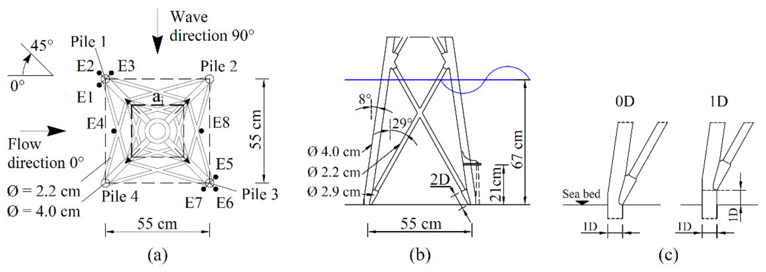
  • To investigate the influence of vertical structural elements (i.e., structural distance of the lowest node to the seabed) on the time-dependent local scour development, local equilibrium scour depth and local spatial differences around the main piles.
  • To propose improved prediction methods and discuss design recommendations for jacket-type offshore foundations.
  • To analyze and quantify differences of displaced sediment volumes, incrementally and cumulatively, to investigate the influence of the distance of the lowest node to the seabed on erosion and deposition patterns around the foundation structure.
  • To quantify the spatial volume change of displaced sediment per surface area, which exhibit an increased erosion or deposition of sediment, potentially affecting benthic flora and fauna.

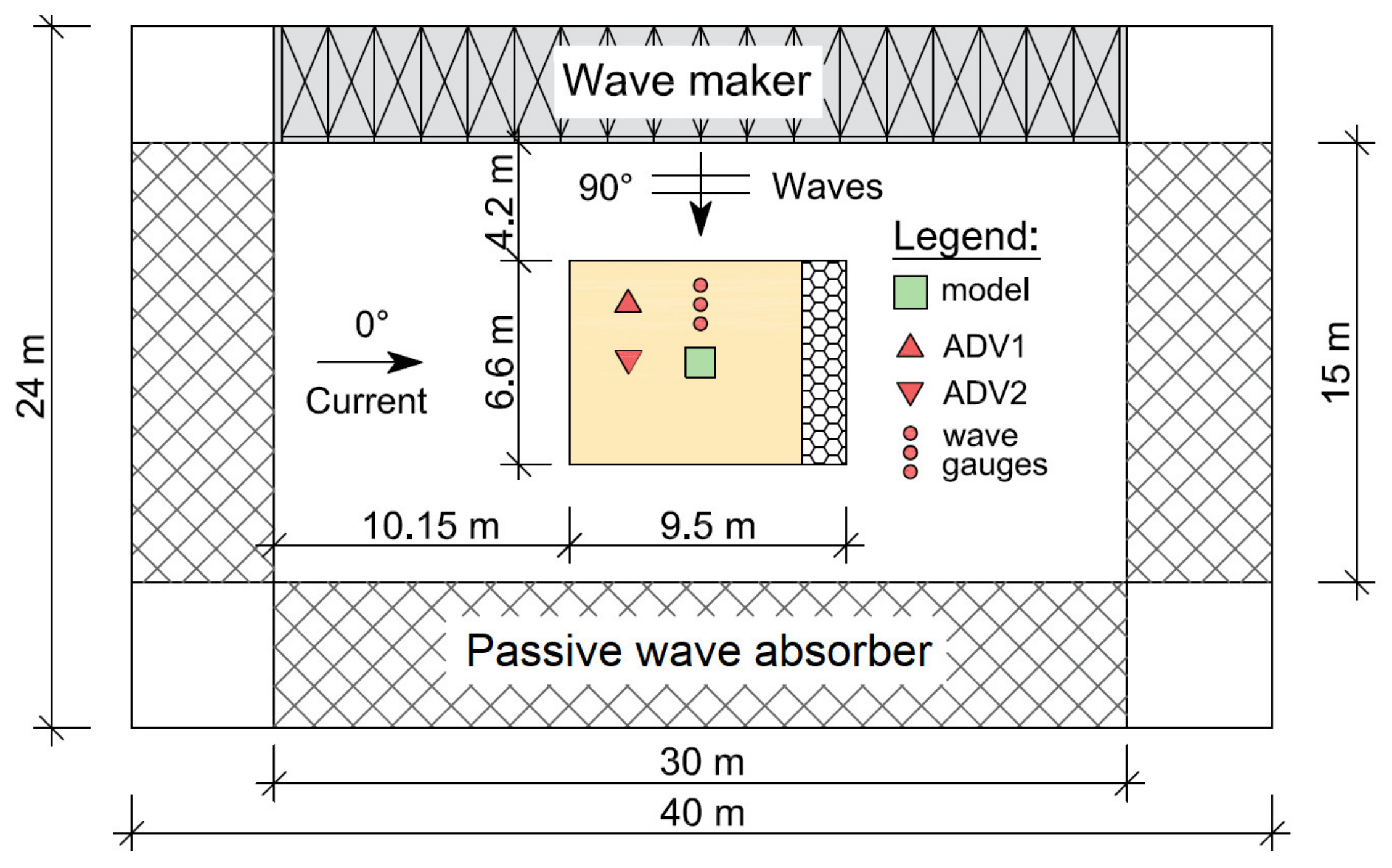
2. Experimental Setup

This study represents an extended analysis of model tests initially described in Welzel et al. [35]. Furthermore, the experimental setup and test procedure of the present study is similar to the one described in References [24,34]. Information on the experimental layout and methodology is summarized in the following paragraph, but more detailed information about the test setup and procedure can be found in [24,34]. The 3D wave basin used for this study has a total length of 40 m and a width of 24 m, as well as a maximum water depth of about 1 m (see Figure 1). An in-depth description of the wave basin features is available through the recent work of Schendel [36]. A sediment pit is placed in the middle of the basin, with a length of 8 m, a width of 6.6 m and an additional depth of 1.2 m, assuring that a sufficient soil layer is available for wave-induced transient pressure waves to freely propagate in half-space. A sediment trap (length of 1.5 m in current direction) is placed at the downstream side of the sediment pit, which was installed to prevent large sediment transport as bed load into the pump sump. Reflections are effectively reduced with a wave maker-integrated active and an additional passive wave-absorption system. The steady current is approaching from left to right, which is corresponding to 0° (see Figure 1). The direction of waves was set at 90° for comparability reasons, as well as to study the impact of perpendicular approaching waves on the scour development. For the physical model tests a jacket-type model was designed, which consists of 3D-printed elements, assembled and joined together by 2-component glue; a surface finish with filler and lacquer in multiple layers was applied to achieve a smooth, high-quality surface.
Assuming a model length scale of 1:30, a constant water level of 0.67 m was maintained during the tests, which corresponds to a water level of about 20 m in prototype dimension (see Figure 2). The jacket model has a quadratic footprint with a spacing between the main piles of 0.55 m, with a diameter of 4 cm and diagonal braces with a diameter of 2.2 cm. Distances along the x-axis and y-axis are given in this study as multiples of a dimensionless parameter “A”, which relates the distances along x and y to the edge length of the structure’s footprint (A = x or y distance/structure footprint distance; e.g., 0.5A = 0.275 m/0.55 m). For the tests, a crystal quartz sand with a median diameter of d50 = 0.19 mm was used. The sand was installed in wet conditions, in order to achieve good compaction. The wave spectra were measured with an array of ultrasonic wave gauges (General Acoustics, ULS HF 58, Kiel, Germany), measuring with a frequency of 200 Hz (see Figure 2). Flow velocities, induced by waves and currents, were measured with two Acoustic Doppler Velocimeter, installed vertically with the x-axis pointing in current direction (ADV, Vectrino + from Nortek, Norway). ADV1 was installed in the axis of the wave gauge array, and ADV2 in the middle of the current generation side in a distance of 2.5 m from the center of the model. The velocities were measured in a distance of 10 cm above the seabed (10 cm = 2.5D). The undisturbed current, Uc, and orbital, Um, velocity, as well as the depth averaged current velocity, U, were measured during preliminary tests. The Ultrasonic Ranging System (URS from Seatek) consists of small echo sounding devices with a diameter of 1 cm per sensor, (configured measuring frequency = 1 Hz). The small size of the sensors allows underwater in situ measurements, which enabled a continuous scour depth measurement over time at eight positions around the complex structure. The devices were installed 21 cm (21 cm ≈ 5D) above the bed, in a distance of 1 cm next to the piles around Pile 1 (E1–E3) and Pile 3 (E5–E7), to measure the local scour development over time on the upstream and downstream side of the structure (with respect to the current direction). Insights about the global scour development, as an effect of the structure, are additionally given with two echo sounders (E4 and E8) placed between the upstream and downstream piles (see Figure 2). The detailed 3D surface elevation was measured with a terrestrial 3D laser scanner (FARO Focus). The laser scanner provides a high resolution of up to 1 mm grid size, resulting in up to 70 million data points per scan. Interrogation areas, ai, starting in the center of the structure or at each individual pile, increasing up to 6.5 times the structure footprint size (6.5A), are used in the present study, to analyze the change of sediment volume in a spatial reference. In order to investigate and assess the influence of the distance of the lowest node to the seabed, the physical model was constructed with an adjustable pile foundation. By means of this feature, the distance of the lowest nodes to the seabed could be adjusted to study its effects. In the present study, the model was installed with the lowest node ending directly on the seabed surface (following defined as 0D; see Figure 2c), to compare measurements of the present study with data measured under the same conditions, in a distance of 1D to the lowest node. The position of the node at 0D was chosen as a comparison case for the tests with a distance of 1D in References [24,34].
We aimed to, on the one hand, preferably investigate a significant difference (assuming that structural elements close to the seabed generally induce an increased erosion of sediment), and on the other hand, reveal and quantify differences of displaced sediment for a small but significant change in the structural design. Based on this comparison, first qualitative recommendations pertaining to the effect of structural member distance to the seafloor can be given.

Experimental Procedure and Test Conditions

Prior to each test series, the sediment bed was smoothed under wet conditions with aluminum bars. Subsequently, water was filled into the wave basin overnight. JONSWAP wave spectra of approximately 650 waves were generated. After 650 waves, a pause of about 10 min was conducted to calm down the disturbances due to the waves in the basin. The spectra were repeated 10 times for each test, until a maximum amount of 6500 waves was reached. As Tests 1–3, Tests 4 and 5 were conducted with different wave spectra, the test durations differ (KC = 6.7~220 min per test, KC = 14.9~390 min per test). In summary, the test procedure was as follows:
  • Smoothing the sand bed under wet conditions.
  • Measuring of pre-scans and filling the wave basin.
  • Running the desired wave spectrum with the smallest velocity, Uc, of the test series.
  • Increasing the current velocity to the next larger velocity value and repeating Step 3.
  • Increasing the current velocity to the highest velocity and repeating Step 3.
  • Slowly emptying the wave basin and carefully draining the sand pit.
  • Measuring of post-scans.
The undisturbed orbital velocity Um is calculated as follows:
U m = 2 U r m s
U r m s 2 = 0 S f d f
where Urms is the root-mean-square (RMS) value of the orbital velocity, U, at the seabed in direction of the waves, and S(f) = power spectrum of U, corresponding to the wave component, with f = frequency. The Keulegan–Carpenter number was defined after Reference [20] as KC = (Um × Tp)/D with KC = 6.7 and 14.9, in which Tp = peak wave period, and D = pile diameter. The parameter Uc represents the undisturbed steady current velocity in a distance of 10 cm close to the bed. The velocity ratio Ucw represents a ratio between Uc and Um, in the range of 0.37 < Ucw < 0.75. The tests of the present study (see Table 1, T1–5, 0D) involve the nodes starting directly on the level of the sediment bed. Tests conducted within Reference [24,34] were conducted with a distance between the lowest node and the seabed of 1D and are listed additionally in Table 1, T1–5, 1D. The mean value of echo sounder E1–E3 was used as scour depth around Pile 1 (located at the upstream side in current direction). Echo sounder probes E5–E7 provide representative mean scour depths for Pile 3 (see Table 1). In the present study, a final scour depth, Send, was used as the mean value of the last 25% of each test. This percentage was chosen in relation to the fluctuation period of the signal, similar as introduced in Reference [24].
For both studied node distances, 3D laser scans of the seabed were conducted for Test 3 and Test 5. Welzel et al. [34] introduced different volume analyzing approaches, which are used and adapted in the present study, to investigate and assess complex erosion and deposition patterns in the near- and far-field of the offshore foundation. These approaches are, hence, only briefly introduced, as a detailed introduction and discussion is given in Reference [34]. The application of those approaches is not limited to offshore foundations, as used in this study, but can also be adapted, for example, to analyze erosion patterns for bridge piers in rivers. Any spatial measurement technique might be used to generate a digital elevation model (DEM), enabling the utilization of the introduced techniques.
The “displaced sediment volume” (Vi), is defined for the present study as the change of sediment volume related to each specific area ai.
V i = Z i a i × A g
where Z i a i is the sum of elevation differences, Z, between the pre- and post-scan calculated for each interpolated grid point (Welzel et al. [34]) and within the area ai and Ag the area related to one datapoint, depending on the grid resolution of the 3D scan.
In the following paragraphs, Section 3.1 and Section 3.3, the parameter Vi denotes a “displaced net volume”, including eroded and deposited sediment volume (Vi = Vdeposition + Verosion). Section 3.4 focuses on deposition patterns; here, Vi represents only the “volume of deposited sediment” (Vi = Vdeposition). Similar to those introduced in Reference [34], two parameters, DA,i and DI,i, are used to calculate an erosion or deposition depth, based on the relation of displaced volume and the related interrogation area, ai. As discussed in Reference [34], a normalization strategy should be chosen in relation to the geometric properties of the foundation directly obstructing the flow at the interface and within the soil. In this study, the diameter (D) of each main pile of the jacket structure is used to normalize DA,i and DI,i, as the local and global erosion process around a jacket structure is found to be mainly controlled by the diameter of the piles. These parameters give information on the relative volume change per surface area, in the following summarized as “erosion or deposition intensity”. Furthermore, the chosen normalization strategy enables a direct comparison between displaced sediment volume related to a specific area and scour depths or bathymetric data.
The “cumulative volume depth” (DA,i)sets a volume (Vi) in relation to the interrogation area (ai) and is further normalized by the main pile’s diameter. This representation reveals the relative volume change per total surface area ai for each value of DA,i.
D A , i = V i a i / D
The “incremental volume depth” (DI,i) represents the relative volume change per surface area of an individual volume ViVi−1 within adjacent areas aiai−1. As displaced sediment volumes for areas aiai−1 are considered in a spatial resolution within and around the foundation structure, the actual complex shape of the considered erosion or deposition pattern can be calculated and described with few parameters.
D I , i = V i V i 1 a i a i 1 / D

3. Results

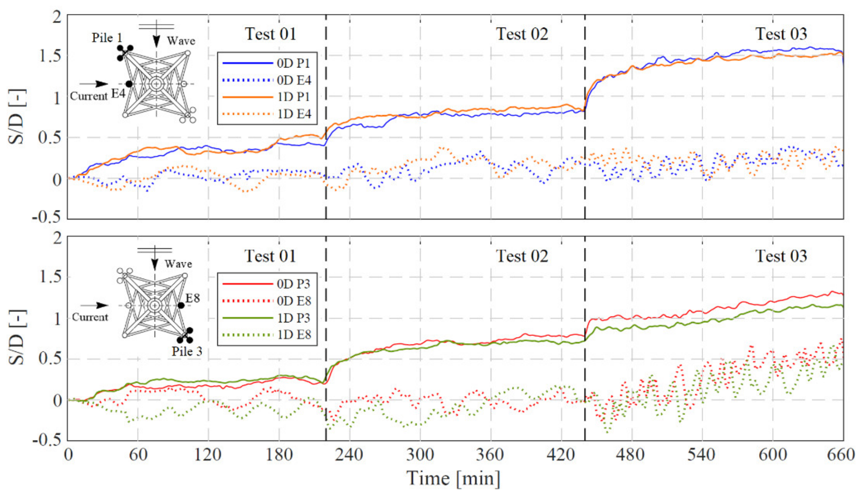
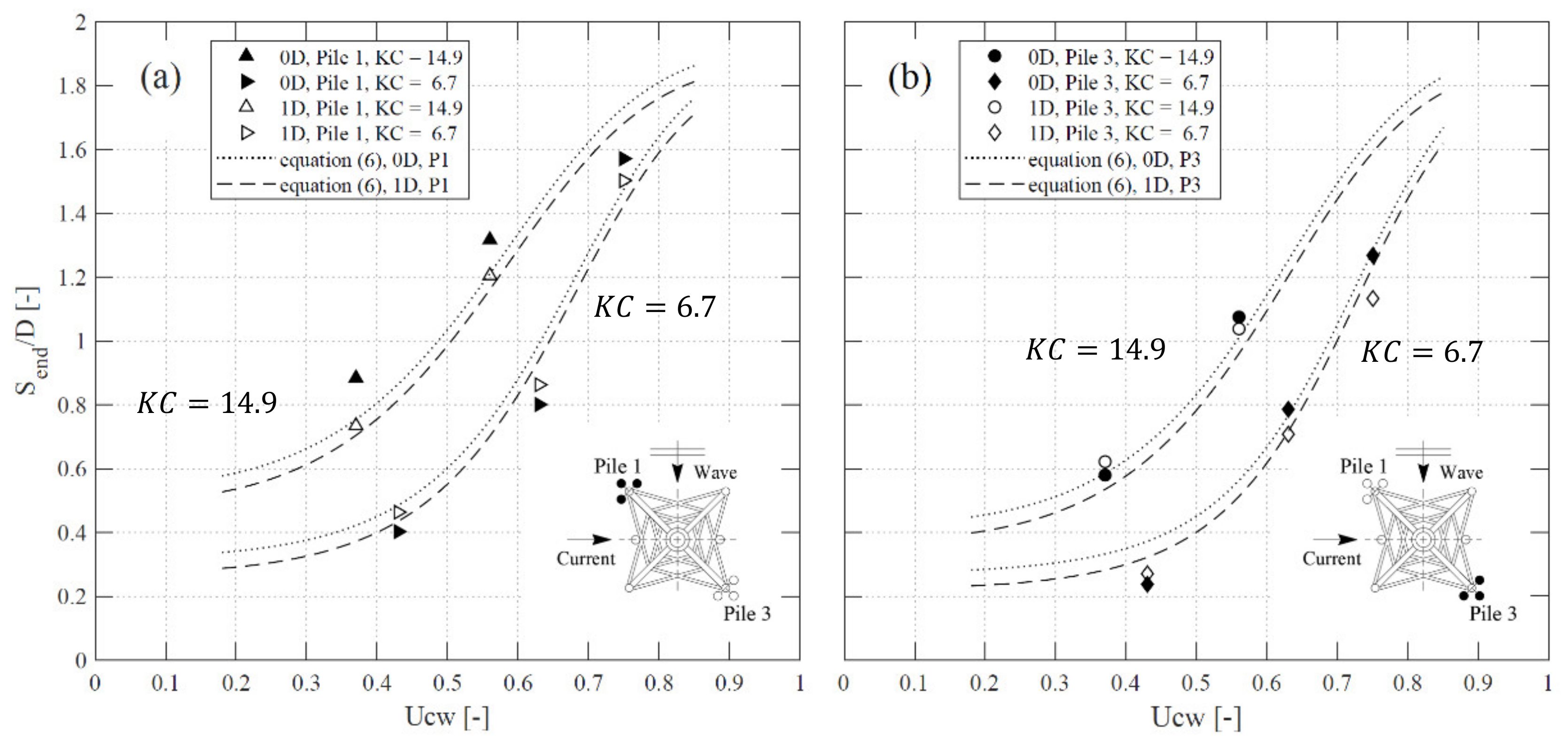
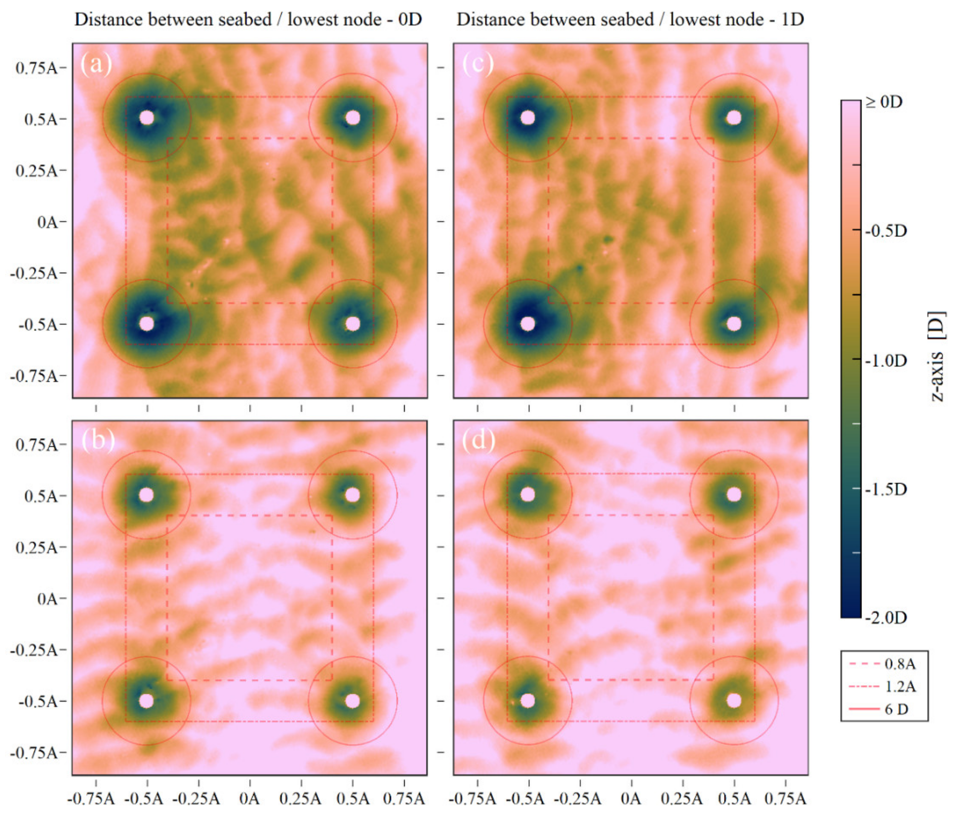
3.1. Development and Final Scour Depth around the Main Piles
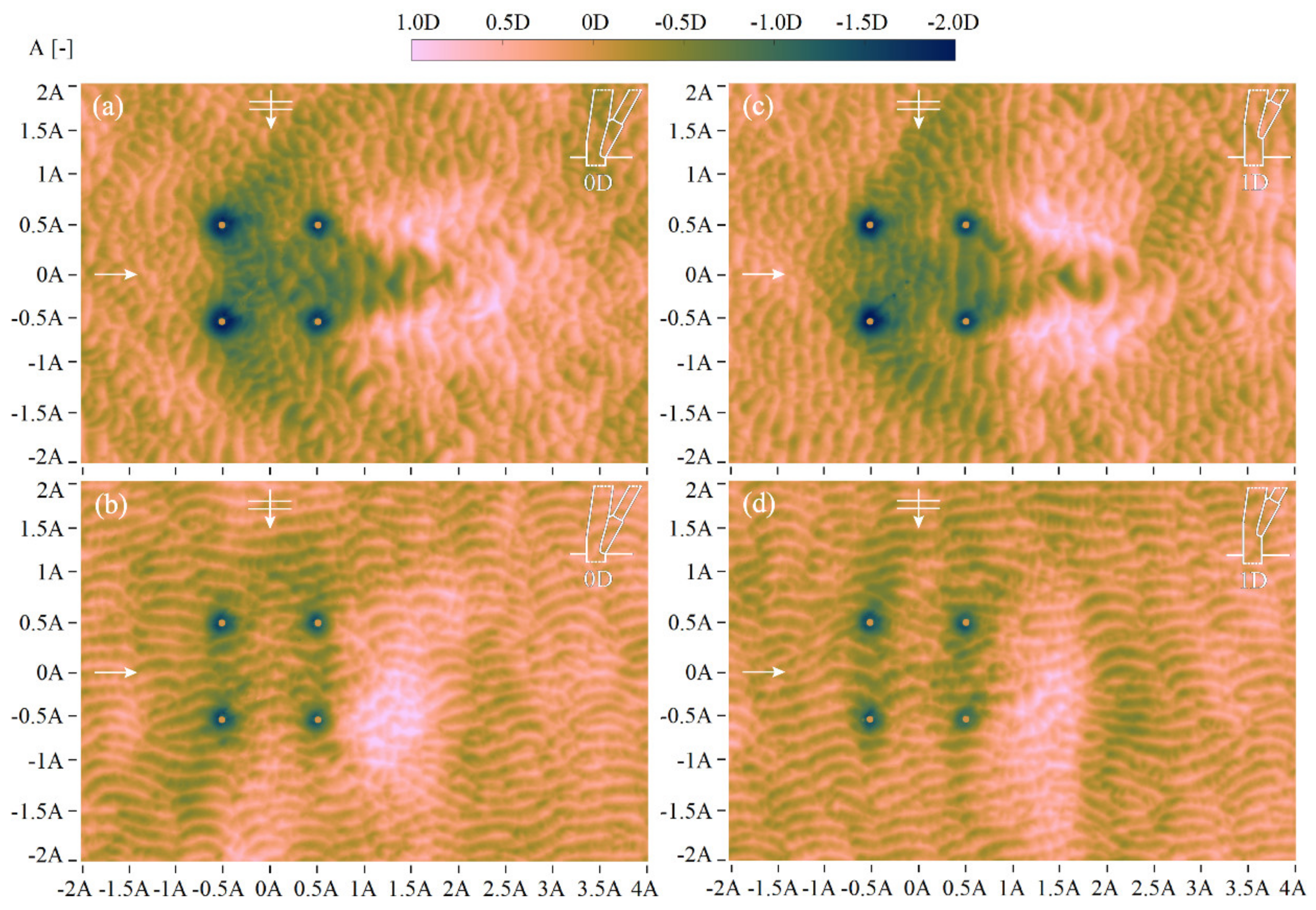
The time-dependent scour development of Tests 1–3, 0D is illustrated in Figure 3 and compared with measurements for a 1D node distance, but with otherwise identical hydraulic conditions. While the echo sounders measured around the piles, but not directly under the braces (see Figure 2), the scour depths at these points were still influenced indirectly from the lowered structure. The flow on the downstream side of the structure (see bottom picture, Figure 3) was affected by structural elements located on the upstream side (top picture, Figure 3) of the structure and thus led to a lower scour depth around Pile 3, combined with a more pronounced global scour depth at position E8 (see transducer E8, Figure 3).
The time-dependent signal of transducer E4 and E8 (for both cases 0D and 1D node distance) is additionally presented in Figure 3. Transducer E4 and E8 measured a more globally affected scour depth in between Piles 1 and 4 (E4, on the upstream side) and between Piles 2 and 3 (E8, downstream side). These locations are characterized by complex hydrodynamic conditions. Streamline contraction, combined with vortices induced by the surrounding structural elements, affects the sediment transport process, leading to global scour. Thus, the measurements at these locations show a less steady scour depth progression than those directly at the main piles, especially for current-dominated flow conditions. Furthermore, at position E8, the depth of the global scour was almost always larger for a node distance of 0D than for a node distance of 1D. In the current-dominated conditions of Test 3, the scour depth increased similarly for both node distances.
At position E8, it is observed that the globally affected scour depth was larger for a node distance of 0D than for a distance of 1D (Tests 1–3), with a similarly increasing scour depth for current-dominated conditions of Test 3. On the contrary, the differences in scour depth between both node distances are less pronounced at position E4. Measurements of the globally affected scour depth at position E4 and E8 seem to generally follow the observations made for the local scour around Piles 1 and 3. An example is a comparison of the development of E4 and the scour development around Pile 1 in Tests 2 and 3. While a slightly larger scour depth can be observed for Test 2, P1, 1D, the development of E4 for 1D is also slightly increased above E4, 0D. In Test 3, which was conducted with an increased current velocity, this development is inverted as E4; 0D starts with a smaller scour depth than E4, 1D and increases gradually above E4, 0D, similarly to the development of Test 3, P1, 0D, which also increased gradually above P1, 1D. The scour development of Test 1, 0D (Piles 1 and 3; see Figure 3) reveals a slightly lower scour depth, combined with a lower fluctuation than Test 1, 1D. Test 2 shows comparable scour depths for Piles 1 and 3, while measurements of Test 3 indicate a clear influence of the lowered structure, resulting in lower scour depths for a 1D node distance compared to a 0D node distance.
Figure 4 illustrates the normalized final scour, depth Send/D, of each test at both piles on the upstream (Figure 4a, Pile 1) and downstream (Figure 4b, Pile 3) side of the structure for 0D and 1D node distance tests. At the upstream pile (E1–E3, Pile 1), a comparison between the final scour depth for 0D and 1D node distances reveals slightly larger scour depths for KC = 6.7 (Tests 1 and 2) for a 1D node distance, which is unexpected. Only for Test 3 (KC = 6.7), the test with the largest current flow velocity, a slightly larger final scour depth was obtained for a node distance of 0D. Echo sounder probes E5–E7 are located on the downstream side at Pile 3. In general, scour depth on the downstream side is found to be smaller than that on the upstream side of the jacket structure. The comparison of final scour depths between 0D and 1D node distances reveals larger scour depths for KC = 6.7 (Tests 2 and 3) for a 0D node distance. Only Test 1 (KC = 6.7), the test with the smallest current velocity, depicted a larger final scour depth for a node distance of 1D, which again is unexpected. While the current flow velocity in Test 1 alone was not strong enough to initiate the scour process, as the flow intensity was U/Ucrit = 0.39 and thus below the critical threshold for erosion of U/Ucrit = 0.5 as defined by Breuers et al. [17], the current velocity of Test 2 should have been high enough to initiate the scouring process (U/Ucrit = 0.87) by its own. Additionally, the wave boundary layer thickness can be assumed to have been comparably thin for the tests with a small KC number, contributing to generally smaller flow velocities and less consistent vortex systems around the structural elements close to the seabed. In consequence, vortex systems and the contracted flow around the near bed structural elements might have a smaller impact on the scour development for Tests 1 and 2.
However, the scour depths for tests with a large KC = 14.9 (Tests 4 and 5) give a different picture. At the upstream pile (E1–E3, Pile 1), the comparison of final scour depths between 0D and 1D node distances reveals a significant increased (ΔSend/D = 0.15, Test 4; ΔSend/D = 0.11, Test 5) scour depth for a 0D node distance. The present results indicate an influence of the node distance on the scouring process, mainly expressed as a different dependence on the KC number. At the downstream pile (E5–E7, Pile 3), differences between 0D and 1D node distances are comparable small (ΔSend/D = 0.04, for Tests 4 and 5). Scour depths for a 0D node distance at Pile 3, for KC = 6.7 and 14.9, were smaller than those for a 1D node distance as long as the current flow component was relatively small (Ucw < 0.5). Thus, measurements of the present study at Pile 3 indicate that differences in scour depth between a 0D and 1D node distance are mainly influenced by the current flow component.
An equation for the prediction of scour depths at a jacket foundation in combined wave and current conditions is proposed that differentiates between the upstream (A = Afront) and downstream (A = Arear) side of the structure and additionally considers the distance of the lowest node from the seabed. To consider the influence of the node distance, the coefficient B is included, with B = 0.17 for a node distance of 1D and B = 0.22 for a node distance of 0D. Compare this to the approach for the prediction of scour depths at a jacket structure that was introduced in Reference [24].
S e n d D = 0.7 + e x p 6.5 U c w 2.5 A 1.5 + B
with
A f r o n t = 1.66 K C 0.34 4.5
A r e a r = 1.30 K C 0.40 4.6
Although Test 1 (Ucw = 0.43, KC = 6.7), 2 (Ucw = 0.63, KC = 6.7) and 4 (Ucw = 0.37, KC = 14.9) partially reveal lower scour depths for a 0D node distance, an acceptable prediction value (improved R² from R² = 0.89 to R² = 0.91 for 0D scour depths) with less underpredicted scour depths is reached in general for Tests 1–5 with the adjusted term in Equation (6). The comparison of final scour depths, therefore, indicates a less pronounced influence of the structural design for lower KC and Ucw values and a slightly more pronounced impact of the distance to the lowest node for higher KC values and current-dominated hydrodynamic conditions.
In the following section, the local scouring process around the main piles is further analyzed with the parameter DI,i (using Equation (5)), applying increasing circular ring areas around each pile (see for an example inner graphical subset of Figure 5a). The shaded area (depicted within Figure 5a) represents an example of one circular incremental area, ai, whose diameter is given as multiples of D. Each calculated erosion depth, DI,i, is related to one particular incremental area, ai.
As sand is removed by an increased velocity and vorticity around the pile, the local slope angle of the scour hole exceeds the internal friction angle of the sediment, and sediment starts to slide from higher to lower locations. Due to this process, the local scour hole is shaped and deepened, depending on the dominant flow and vortex systems around the structure. On the one hand, DI gives information about the relative volume change per surface area (erosion intensity), the mean surface slope and the mean shape of the analyzed scour holes, but also on the erosion depth, enabling a direct comparison to scour depth values. Figure 5a illustrates the mean development of DI,i for Piles 1–4 and compares 0D measurements with 1D node distance scans. A discussion of analyzed scour holes (also for Tests 3 and 5) in 1D node distance is given in [34].
It is not completely clear whether the first measurement point close to the pile (located at 1.5D) might be affected by boundary effects during the drainage of the water or by an interference of the 3D laser scanner with the pile of the structure. Therefore, the first data point is disregarded in the following comparison between present measurements for 0D and 1D node distances. Differences in the erosion depth of DI,i between both node distances are as follows:
Δ D I , i = D I , 0 D D I , 1 D
Figure 5b reveals differences in the mean erosion depth, ΔDI, for Piles 1–4. Positive values of ΔDI indicate a higher local erosion for tests with a node distance of 1D, whereas negative values indicate a higher local erosion for tests with a 0D node distance. Figure 5a shows that the extent of the local scour hole reaches up to a radial distance of about 6D for Test 3 and a distance of about 5D for Test 5. This difference in radial extent of the scour hole between the tests is expected, considering the smaller flow velocity and consequently smaller final scour depth at the pile in Test 5. With respect to the radial extent of the scour hole, no significant difference between a 0D and a 1D node distance was observed for Test 5. However, a comparison between Test 3 for 0D and 1D node distance revealed a flattened scour hole slope with a slightly larger extent for a 0D node distance. Nevertheless, larger erosion depths, DI, were calculated for a node distance of 0D, especially for Test 3. An exception to this is the measurement point closest to the pile where the erosion depth for both node distances is similar (radial distance of 2D) or higher (radial distance of 1.5D) for a node distance of 1D.
Figure 5b clearly shows that additional sediment volume was eroded due to the smaller node distance mainly at a radial distance of 2.5D–7D for Test 3, leading to a flattened scour hole slope for a 0D node distance for Piles 1–4. In contrast, for Test 5, larger scour depths due to a smaller node distance were only measured up to a radial distance of 2D–5D, leading to a steeper scour hole slope for a 0D node distance for Piles 1–4. From these distances on (8D for Test 3 and 6D for Test 5), the influence of the lowered node on the scouring process seems to be reduced notable. Furthermore, it is noted that a direct comparison between the erosion depth, DI, and final scour depth, Send/D, might be misleading and therefore not appropriate, as different measurement and analyzing techniques are utilized (see Section 4.2 for a detailed discussion).

3.2. Bed Topography

Laser scans were conducted after each test series (see previously described test procedure). Based on these scans, Figure 6 presents the bed topography after Tests 3 and 5. Here, Figure 6a,b shows the bed topography for a node distance of 0D, while Figure 6c,d shows the bed topography for a node distance of 1D. The steady current is coming from left to right (0°) in all figures, while incident waves were coming from 90°, perpendicular to the current. Erosion of sediment is illustrated in dark blue and green colors, while a light brown color represents the transition to deposed sediment. Test 3 (Figure 6a) was conducted under current-dominated conditions (Um = 13.3 cm/s, Uc = 38.8 cm/s, Ucw = 0.75), which led to sand ripples with comparable long crests and smaller heights (cp. ripples under steady current conditions [34]) migrating in current direction. The bed topography shown in Figure 6a illustrates global sediment transport processes characterized by erosion underneath and in the near-field of the structure and deposition on the downstream side of the structure. The globally eroded sediment led to scour depths of approximately 0.7D in between the structure footprint (within a distance ≤ 1A). In flow direction laterally to the structure, erosion areas emerged from Piles 1, 3 and 4, potentially indicating amplified vortex shedding from the sides of the jacket structure due its blockage effect. In contrast to Test 3, Test 5 (Figure 6b) reveals a sand ripple migration with long crests in wave direction, as a result of the higher orbital velocity (Um = 17.5 cm/s, KC = 14.9), and a lower current velocity (Uc = 22.5 cm/s), which led to a wave current velocity ratio of Ucw = 0.56. The 3D scan measured after Test 5 (see Figure 6b) shows the eroded and deposed areas as a result of the hydrodynamic conditions after a time period of 390 min (6500 waves).
The scan of Test 5 reveals locally eroded sediment around the piles and a comparable low global erosion in the near-field of the structure, which led to global scour depths in the range of 0.2–0.4D, in between the structure footprint. As a consequence of a lower current velocity and higher orbital velocity, deposition of sediment is allocated on the lee side of the structure, in current direction, in a closer distance as compared to Test 3. For a node distance of 1D (Figure 6c,d), erosion and deposition patterns around the structure look generally similar to that obtained for a node distance of 0D. Besides small differences regarding the deposition patterns, the comparison reveals differences in the laterally eroded areas, which are emerging only from Piles 1 and 4 in Figure 6a,c. As differences in scour depth between a 0D and 1D node distance is visually hard to distinguish, an additional close-up view of the structure’s footprint area is illustrated and discussed in Figure 7.
Figure 7a,b illustrates the bed topography for Tests 3 and 5 for a node distance of 0D, while Figure 7c,d shows the bed topography for a node distance of 1D. In general, the lowered braces (0D node distance) represent an additional obstruction for the flow. The results indicate that the braces led to a change in the near bed flow pattern, in particular for current-dominated flow conditions, resulting in differences in the bed topography. A comparison between the close-up of Figure 7 (a, 0D) and (c, 1D) clearly shows differences in the bed topography after Test 3. Underneath the structure, a deeper areal scour depth extended over a larger area for a node distance of 0D than for 1D. A difference in the scour depth can be observed, in particular, in between the structure footprint (distances < 1A). Additionally, the size of the local scour is increased for Test 3 for a node distance of 0D, compared to 1D (see Figure 7a,c), which was presented and discussed in Figure 5. A circle with a diameter of 6D was added around the piles in Figure 7, to enable a comparison of the spatial extent of each local scour. Test 5 is characterized with increased orbital and decreased current velocities. Contrary to Test 3, a visual difference for the bed topography of Test 5 is not clearly identified in the close-up view. Nevertheless, differences between both tests are clearly revealed by the differential volumes between the 0D and 1D node distance analyzed and discussed in the following paragraph, Section 3.3.

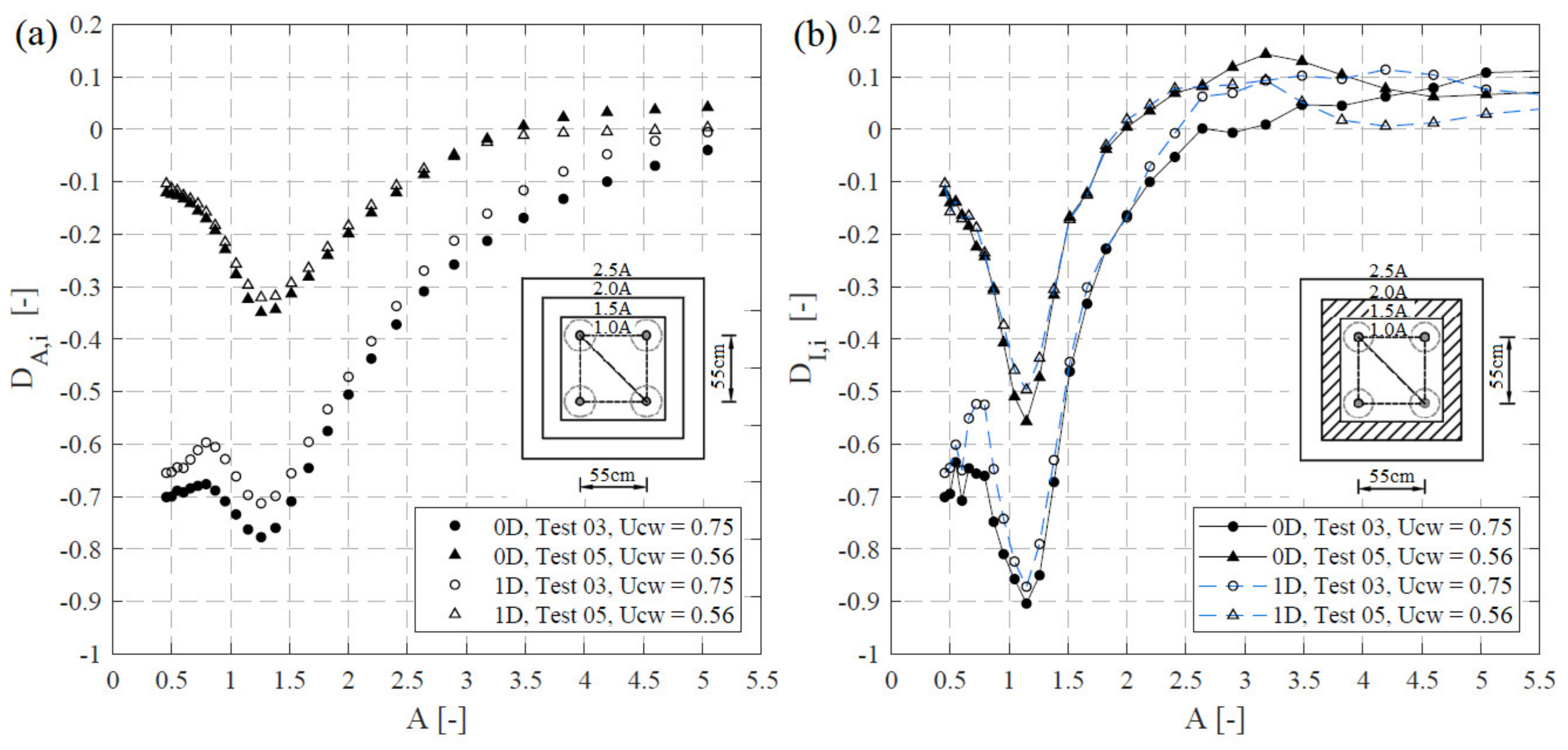
3.3. Influence of the Structural Node Distance on Displaced Net Volume

In Figure 8, the cumulative (DA,i) (Figure 8a) and the incremental (DI,i) (Figure 8b) volume depths (Equations (4) and (5)) are plotted in a spatial reference with the former introduced methodology, to provide a better parameterized description of the effect on the redistribution of sediment around the jacket structure and how it is influenced by a reduction of the node distance. As a consequence of the calculation method, higher erosion intensities and enhanced fluctuations are given by DI,i than by DA,i, since the former represents the erosion depth or deposition value within incremental areas aiai−1, while the latter refers to the entire area, ai. In Figure 8, positive values of DA,i and DI,i refer to a net deposition of sediment volume, whereas negative values show a net erosion of sediment, following the definitions given in Section 2. For both considered tests and node distances, Figure 8 shows a peak of maximum erosion intensity at 1.2–1.25A. Increased erosive gradients, i.e., a steeper development of changes of scour volume per surface area directed from the structure’s center 0.5A to 1.25A, are revealed under the influence of higher orbital velocities (Test 5, Ucw = 0.56), in relation to Test 3 (Ucw = 0.75). This illustrates a more locally pronounced erosion of sediment around the piles (located at about 1–1.25A) for Test 5 than for Test 3, while the sediment displacement in Test 3 was dominated by a more globally pronounced erosion pattern (increased erosion depths for A < 1).
The influence of the node distance increased with increasing current velocity. While only small differences in the amount of eroded sediment in relation to the distance of the structure were measured for Test 5, a clear increase in erosion due to a reduction of the node distance can be seen for Test 3. As expected, the influence of the node was particularly large in the vicinity of the structure (<1.25A), but an influence of the node distance can also be found at greater distances of more than 3A. For further evaluation of the influence of the node distance on the spatial sediment displacement, the differences in cumulative (DA,i) and incremental (DI,i) erosion depth are directly compared in Figure 9. To this end, erosion depths in tests with a 0D node distance are subtracted from those obtained in test with a 1D node distance.
Positive values in Figure 9 refer to higher magnitudes of net erosion for a 1D node distance, while negative values refer to a higher net erosion for a 0D node distance. Generally, Figure 9 confirms the anticipated effect that more sediment gets eroded due to a closer node distance up to a distance from the structure of 2.5A. It is notable that the erosion intensity of Test 5, 0D is increased up to a distance of about 2–2.5 times (Figure 9b) the structure footprint length, which apparently also marks a reverse with an increased net erosion for Test 5, 1D for distances >2.5A (see Figure 9b). In consequence, differences in the redistribution of sediment above ~2.5A are mainly addressed to deposition patterns on the lee side of the structure. A comparison of the deposition patterns of Tests 3 and 5 revealed significant differences between the 0D and 1D tests. The results of the present study show an influence of the foundation structure for deposition patterns of up to 6.5 times the structure footprint length (see Section 3.4). The present study quantifies the spatial volume change and extent of complex erosion and deposition patterns, highlighting areas and distances in relation to the OWF foundation footprint, potentially affecting benthic flora and fauna.
A closer view on distances on up to 2A reveals differences in erosion patterns directly influenced by the structure. The mobile seabed beneath the jacket structure responds very sensitive to velocity alterations due to the closer distance of the structure to the seabed. The results indicate, although direct measurements of the flow field beneath the structure were not carried out, that the lowered node and diagonal braces cause additional flow compression and near bed vortices, which, in turn, induce higher erosive potentials, especially in between the structure footprint area. Since the braces of the structure are lowered to 0D, it is likely that an additional disturbance of the flow induces an increased sediment mobilization. Figure 9a,b reveals a peak of erosion depth difference at a distance of about 0.8A for Test 3 and at 1.2A for Test 5. The development of the spatially averaged erosion depth generally has a maximum around the piles (located at about 1.2–1.25A, see Figure 9), where the global scour superimposes with locally eroded sediment around the piles. Test 3 has a wave current velocity ratio of Ucw = 0.75, and thus, a current-dominated flow condition. In Figure 9, Test 3 therefore shows that a closer distance of the node from the seabed led to a slightly increased erosion of sediment around the main piles (1.2A). However, the majority of increased erosion was located in between the structure footprint at about 0.8A (see Figure 7 and Figure 9). A slightly increased erosion depth (DA or DI) is found due to the more wave induced flow conditions of Test 5 (Ucw = 0.56). The comparison of erosion depth between a 0D and 1D node in Test 5 shows a slightly increased peak of eroded sediment around the main piles (located at about 1.2 times the structure footprint length). This might be explained by a less dominant current velocity, leading to less pronounced vortices and streamline compression induced by the diagonal braces, which are crossing the current in an angle of about 100 degree.
Furthermore, the comparison between both node distances for Test 3 demonstrates that even a reduction of the node distance by one diameter can have a significant impact on the erosion intensity of sediment in the near-field of the foundation structure. In fact, differences of the incremental volume depth reveal an increase of ΔDI of up to 0.14 diameters (increase of 26%) in a distance of 0.8A for tests conducted in 0D node distance. Therefore, findings related to the visualized differences of Test 3 (see Figure 7) can be generally confirmed as a deeper bed topography can be identified in between the structure footprint (in particular in the 0.8A area). In addition, Figure 7 also shows the border of an interrogation area with a size of 1.2 times the structure footprint (1.2A). However, a deeper local scour depth of Test 5 is visually hard to distinguish in Figure 7, but the analyses reveals a growth of the incremental erosion depth, ΔDI, of up to 0.06 diameters (increase of 12%) in a distance of 1.2A.

3.4. Analysis of Deposition Patterns

To analyze and identify structurally induced deposition patterns of sediment on the lee side of the foundation structure, the incremental volume depth (DI,i) is utilized by using only deposited volume Vi = Vdeposition. The redistributed sediment volume related to the blockage of the foundation structure and the associated net deposition is the focus of the following analysis, revealing areas and distances in relation to the OWF foundation footprint, potentially affecting benthic flora and fauna. Due to the unidirectional current approaching constantly from 0° (see Figure 1), deposition patterns are located for Tests 3 and 5 behind the foundation structure on the lee side (looking in current direction). Figure 10 shows the analyzed deposition volume for interrogation areas aiai−1, starting in the center of the structure, with areas increasing in downstream direction (see graphical subset of Figure 10). These areas, ai, have a rectangular shape (length of 1.5 times the length of the width), to correctly capture the extent of the deposition patterns. To consider that DI,i incorporates sediment volume of ripples (as the sediment bed of each pre-scan was smoothed), a related uninfluenced value is calculated and visualized in Figure 10a. An average ripple deposition value of DI = 0.047 was calculated (sediment volume above the pre-scan due to a natural ripple migration) for an area of 0.5 × 1.0 m, uninfluenced by any streamline contraction or vortices induced by the foundation structure for Tests 3 and 5. To allow for a better comparison and assessment of the generalized development of the deposition intensity induced by the foundation structure, D I * is additionally introduced.
D I * = A m i n A m a x D I , i A r i p p l e   d e p o s i t i o n   d A
To account for the deposition, primary induced by the blockage of the foundation structure, a net deposition value is used in Equation (8), subtracting the “uninfluenced ripple deposition” value from DI,i. This additionally enables to identify differences in gradients of the generalized deposition intensity as the different slopes and angles are related to maxima and minima of the course of DI. The decay curve of deposited sediment volume is analyzed by calculating the cumulative integral of DI from A m i n = 0 up to A m a x 6.5. The limitation of A m a x 6.5 can be explained with the border of the test section, the border of the sediment pit of the wave basin. Figure 10b illustrates the cumulative integral of the net deposition, revealing and differentiating areas with a comparable high deposition intensity (steep gradients) closer to the foundation structure with areas related to a lower deposition intensity (flat gradient). The graph shown in Figure 10b also gives indirect information regarding the total amount of deposited sediment, as well as if the deposition intensity is still increased in reference to an uninfluenced area with natural dynamics of the ocean floor (in this study an uninfluenced test section). In this sense, the course of the cumulative integral should converge to a horizontal line if the deposition volume is decreased on a magnitude of the reference level of the unaffected seabed environment.
In Figure 10a, Test 3 reveals a spatial peak of deposited sediment volume at 2A for 1D node distance, as well as a maximum at 2.4A for the 0D node distance. The majority of deposited sediment volume of Test 3 for a 1D node distance was distributed over a distance of 1.7 times the structure footprint distance (1.7A, 1.3A–3A) from the center of the structure. In case of a node in a distance of 0D to the seabed, the main share of deposited sediment was distributed over a larger distance of 2.1A (1.4–3.5A from the center). This can also be observed in Figure 10b; the end of each main share of deposited sediment is marked by a decrease in the angle of the slope of each test (see 3.5A, Test 3, 0D; 3A, Test 3, 1D). However, we can also observe that fluctuations of the course shown in Figure 10a (Test 3, 1D) are leading to a second increase of the gradient of deposited sediment in Figure 10b.
In Test 5, the peak of volume depth emerged at the same distance from the structure, i.e., 1.6A, for both node distances. The main share of deposited sediment volume related to Test 5, 1D extends over a distance of 1A (1A to 2A from the center of the structure), whereas Test 5, 0D resulted in a deposition of sediment of the main share, elongated over a larger distance, of 1.5A (1.5 times structure footprint distance, 0.9A–2.4A from the center).
Figure 10b clearly shows the decrease of deposited sediment for Test 5. While a structure closer to the seabed (Figure 10b, Test 5, 0D) shows a considerable remaining intensity (relative sediment volume per surface area) of deposited sediment (see 2.2A, Test 5, 0D), a larger distance of the node (Figure 10b, Test 5, 1D) from the seabed leads to a clear decrease of deposited sediment, revealed by a flattened gradient of D I * (see 2A for Test 5, 1D). Nevertheless, a second increase of the gradient for Test 5, 1D can also be observed, indicating that deposition of sediment is still increasing above the uninfluenced reference level (see Figure 10b; 4A). As Figure 10b depicts the cumulative integral of Test 5, 0D, it also shows that D I * is capable of revealing smaller deviations, which are not clearly evident from Figure 10a.

4. Discussion

4.1. Remarks Regarding the Influence of Structural Elements on Scour Depth

The present work was conducted for a jacket structure with comparable large diagonal braces (0.55D and 0.73D at the nodes) in relation to previous studies, such as the works [23,37], and with nodes and near bed braces ending directly on the seabed surface. Results were compared with measurements for a 1D node distance, but otherwise identical hydrodynamic conditions. Thus, the foundation structure of the present study represents a jacket that leads to a large streamline contraction of the flow, potentially resulting in an increased flow disturbance and thus increased bed shear stresses. However, while final scour depths around the main piles of the present study are generally larger for a 0D distance, they are still on a comparable level with those obtained for a jacket structure with nodes and diagonal braces at a 1D distance [24]. Final scour depths of the present study are increased above monopile scour depths, but not in order of magnitude as found in Rudolph et al. [23] (3–4 times the predicted monopile scour depth). This underlines that additional erosion might lead to a significant larger scour depth than described in Welzel et al. [24], which could stem from pile groups (post piles/skirt piles combined with structural main piles) and additional near bed elements and braces, but also from a superposition of a global and local scour development.
However, it is pointed out that additional research is required to better understand the influence of different structural elements on the scouring process and to refine and extend prediction approaches and give improved design recommendations. Therefore, future studies should also strive to extend the given variety of parameters, such as different node distances, the angle of diagonal braces, the diameter of braces, main piles and post piles. Furthermore, the superposition and interaction of local and global scour, are possibly also leading to different timescales and equilibrium conditions outlined and discussed in Reference [24], seem to be important research questions which remain unsolved.

4.2. Remarks Regarding Scale Effects

It is remarked that scale effects are present, in particular due to well-known difficulties in geometrical sediment scaling [38]. To evade a cohesive behavior, the sediment was not scaled geometrically according the model scale of 1:30 (see Section 5 in Welzel et al. [34] for further details on the applied scaling). In consequence of the disproportional scaled velocities and sediment, the relatively large-scaled grain sizes (in comparison to the field) presumably led to an overrepresentation of bedload in relation to an underestimated share of suspended load in comparison to field conditions. In addition, the disproportional scaling also led to larger bed forms (e.g., sediment ripples), thus leading to an increased bed roughness and as a result to a boundary layer with an increased thickness affecting the flow conditions, such as, for example, the size of horseshoe vortices. A comparison of ripples uninfluenced by the foundation structure of Tests 3 and 5 with [39,40] shows a similar geometry and indicates a fully developed ripple length and height. According to Sutherland and Whitehouse [41], the sand ripple migration with relatively larger ripples might also lead to an increased sediment transport in comparison to the prototype scale.
Furthermore, the comparison conducted in Reference [34] already showed similar spatial distributions of erosion patterns for prototype conditions measured in different field studies for the same hydrodynamic conditions as the present study. However, to the best of the authors’ knowledge, there are no field studies available, clearly revealing certain deposition patterns in the near- and far-field of jacket-type foundation structures. The overestimated bedload and underestimated suspended load might affect the outcome and comparison of findings regarding deposition patterns for the present study, which has to be investigated in future studies. This seems to be an important research question in the context of potential influences of offshore foundations on the natural environment, which remains unsolved.
In order to compare findings of the present study with field measurements, the temporal stage of the scouring process is important. An extrapolation analysis revealed that Tests 2–5 reached approximately 90% of the extrapolated equilibrium scour depth during the tests. The analysis also led to the conclusion that Test 1 did not fully reached the equilibrium condition. For more detailed information about the applied extrapolation analysis and a discussion on the interaction between global and local scour, we refer to Reference [24].

4.3. Remarks Regarding a Comparison between Echo Sounder and 3D Scan Data

Attention is drawn here to the comparison between the final scour depth Send/D measured with echo sounders and the maximum erosion depth DI (see Figure 5a; radial distance of 2D) generated with 3D scans, which might lead to slightly larger scour depths for the 3D scan measurements. This can be mainly explained with the different measurement techniques. The Ultrasonic Ranging System (URS from Seatek) consists of echo sounding devices with a diameter of about 1 cm per sensor and a half beam angle of 0.9°, leading to a rather small signal footprint of about 2 cm, measured direct close to the pile in the scour hole. In addition, the final scour depth, Send/D, is gained with the last 25% of the signal, as a considerable fluctuation was observed in [24] and the present study. In contrast, the bed topography measured after each test with the terrestrial 3D laser scanner (FARO Focus) provides a high resolution, of up to 1 mm grid size, and is therefore capable of capturing the smallest differences, leading to comparable larger maximum erosion depths analyzed with DI. Therefore, a direct comparison between DI and Send/D does not seem appropriate and might be misleading.

5. Summary and Conclusions

Hydraulic model tests were conducted in the 3D wave and current basin of the Ludwig-Franzius-Institute, with the focus on the influence of the distances of the lowest node connecting pile and braces to the seabed. A position of the jacket structure with the nodes directly ending on the seabed surface (position 0D) have been chosen as a comparison case for measurements in a node distance of one diameter (position 1D) for identical hydrodynamic conditions. Spatiotemporal bed elevation changes were observed point-wisely, with echo sounder transducers on eight positions, aided by spatial measurements conducted with a terrestrial 3D laser scanner, providing high-resolution measurements of the bed topography. The main conclusions can be summarized as follows:
  • A comparison of final scour depths for 0D and 1D node distances reveals the influence of the structural elements, regarding a shorter distance of the lowest nodes and diagonal braces to the seabed on the local scour development. An improved empirical expression (Equation (6)) is proposed to flexibly account for the structural influence of closer nodes to the seabed, differentiating between 0D and 1D node distances. For piles located on the upstream side (Pile 1) a maximal difference of ΔSend/D = 0.15, was observed for a wave current velocity ratio of Ucw = 0.37 and a Keulegan–Carpenter number of KC = 14.9 for Test 4. For Pile 3, located on the downstream side of the structure (in view of the current direction), a maximal difference of ΔSend/D = 0.14 was observed for Ucw = 0.75 and KC = 6.7 of Test 3.
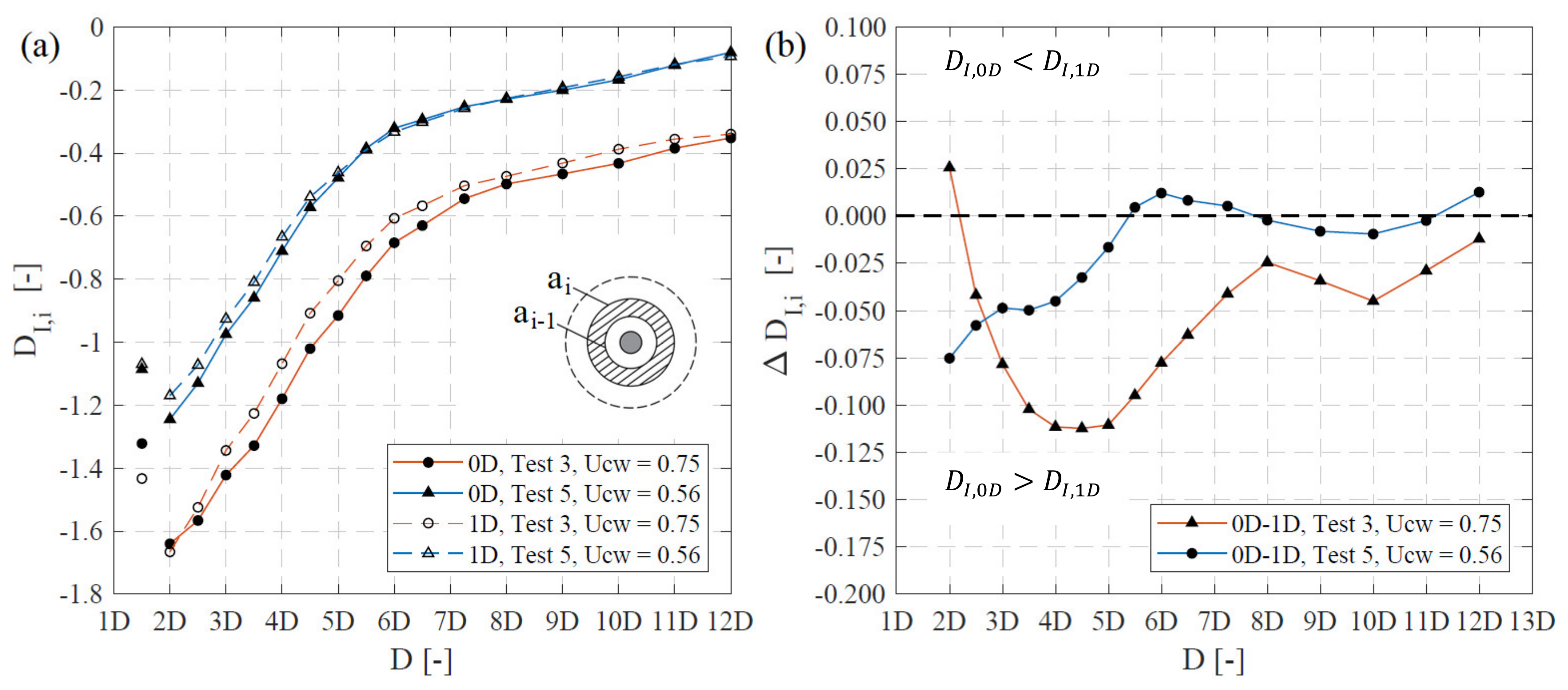
  • Novel analyzing methods have been utilized to reveal spatial volume differences in complex sediment redistribution patterns, enabling a description and quantification of normalized erosion or deposition volumes, as well as a direct comparison between local scour depths and bathymetric data. A comparison of 3D scans with circular areas around each main pile illustrated an increased erosion of sediment for tests conducted in 0D node distance for Piles 1–4. Current-dominated conditions (Ucw = 0.75, Test 3) led to comparable erosion depth at the deepest point, combined with a flattened scour hole slope (for areas with a radial extent of 2.5–7D). Higher orbital and lower current velocities (Ucw = 0.56, Test 5) led to an increased erosion depth (from DI = 1.18, 1D to DI = 1.25, 0D), combined with a steeper scour hole slope, for areas of 2–5D.
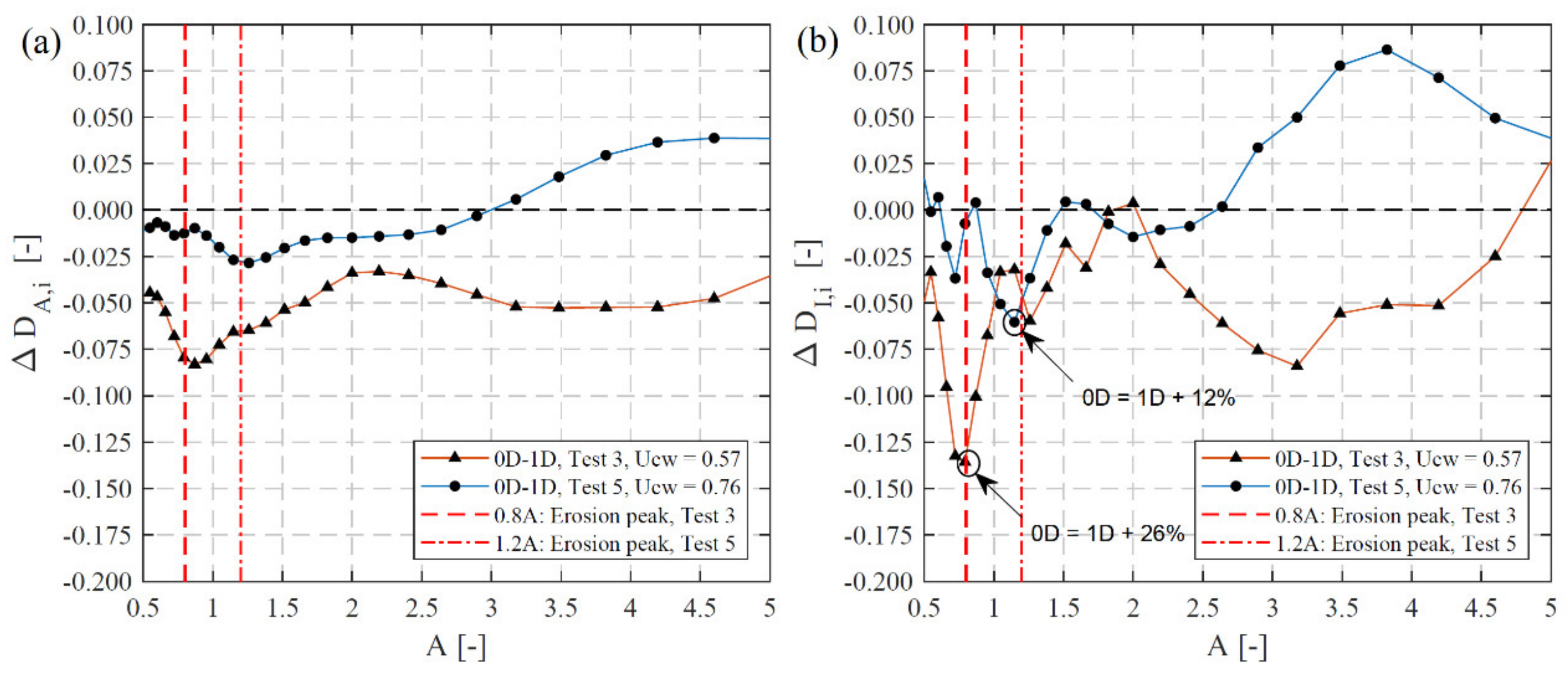
  • The present study reveals that even a small change of the lowest node’s distance from 0D to 1D can have a significant influence on the sediment mobility and displaced sediment volume around an OWF. This highlights the requirement to consider the interaction of the structure with the surrounding seabed within the design process of an OWF not only for reasons of sustainability and economy (reduced scour depth), but also to mitigate impacts on the former unaffected marine environment and benthic habitats due to an increased sediment mobility. The findings indicate that the lowered node and diagonal braces cause additional flow compression and near bed disturbance, which in turn induce a higher spatial erosion, especially in between the structure footprint area for current-dominated conditions, leading to a growth of the incremental volume depth ΔDI of up to 0.14 diameters (increase of 26%, Test 3), as well as a deeper and steeper local scour, but a less globally pronounced erosion for more wave-dominated hydrodynamic conditions, resulting in a growth of ΔDI of up to in 0.06 diameter (increase of 12%, Test 5).
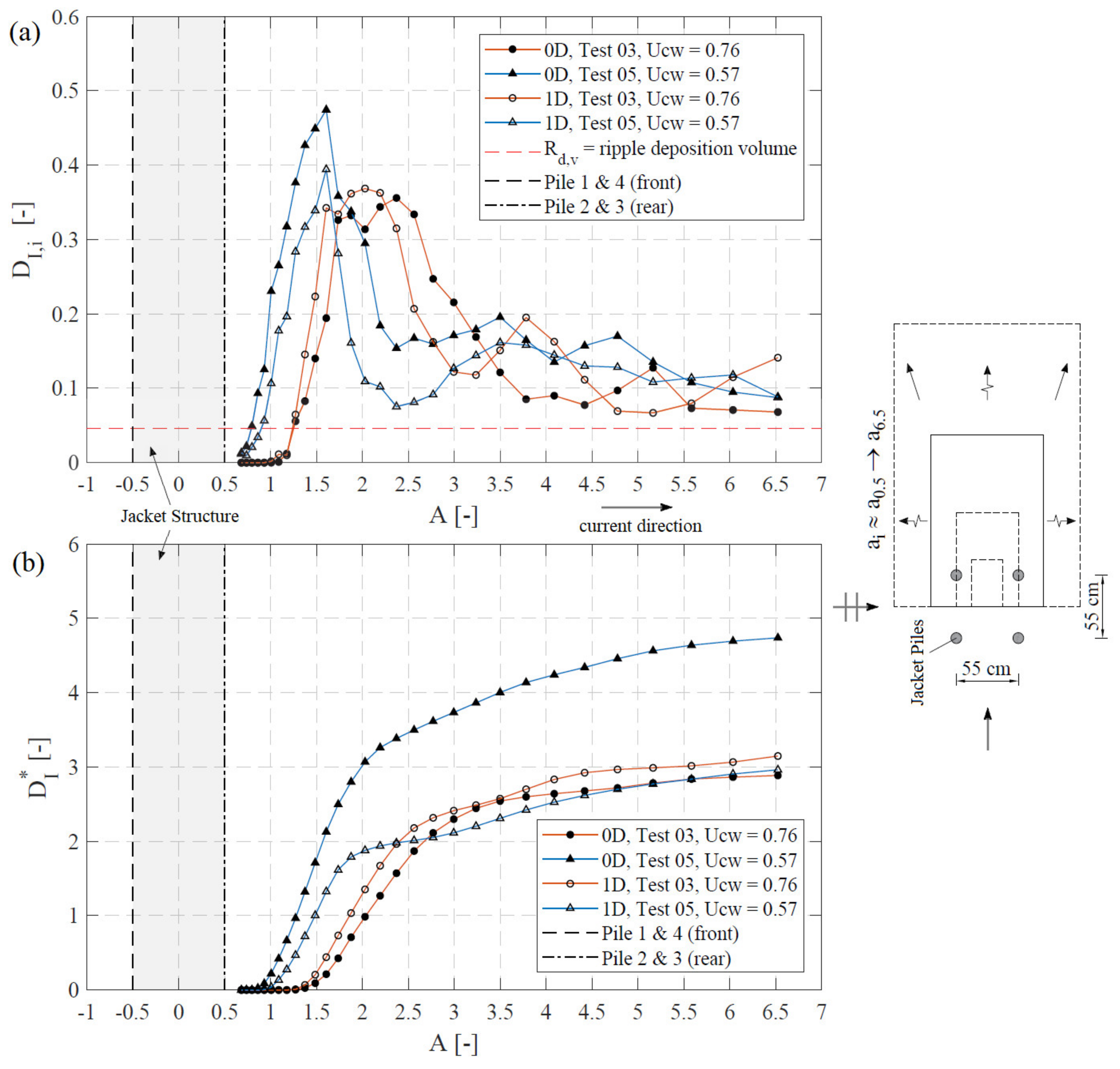
  • Despite an increased erosive potential underneath the structure, the present study also revealed an influence of the foundation structure on deposition patterns over a distance of more than 6.5 times the structure footprint length. Tests with a 0D node distance led to a 24% increased distance of the main share of deposited sediment (2.1A for 0D; 1.7A for 1D) for current-dominated conditions (Test 3), with a spatial offset in current direction but a comparable cumulative deposition volume. However, more wave-dominated conditions (Test 5) led to an increased distance of the deposition pattern of 50% for a 0D node distance (1.5A, 0D and 1A, 1D) combined with an increased cumulative deposition volume.

Author Contributions

For this research article, the specifying of the individual contributions of the authors is as follows: investigation and volume calculations, M.W.; resources, T.S.; writing—original draft preparation, M.W.; writing—review and editing, M.W., A.S., T.S., N.G. and A.H.; supervision, T.S. and A.H.; project administration, T.S. and A.H.; funding acquisition, T.S. All authors have read and agreed to the published version of the manuscript.

Funding

The present study is part of the research project “HyConCast—Hybrid substructure of high strength concrete and ductile iron castings for offshore wind turbines” (BMWI: 0325651A), as well as of the project “marTech-Testing and development of maritime technologies for reliable power supply” (BMWI: 0324196A, 0324196B). The authors gratefully acknowledge the support of the German Federal Ministry for Economic Affairs and Energy within the funded project.

Acknowledgments

The authors gratefully acknowledge the support of T. Kreklow and F. Faltin for their support in conducting the laboratory experiments and preprocessing of the 3D scan data. The authors also thank the FZK, and in particular, M. Miranda-Lange, for support related to the 3D scanner. The perceptually uniform color map batlow Crameri [42] is used in Figure 6 and Figure 7, to prevent visual distortion of the data.

Conflicts of Interest

The authors declare no conflict of interest.

Nomenclature

AReference distance times the structure footprint length;
A = x or y distance/structure footprint distance, e.g., 0.5 A = 0.25 m/0.55 m
aiInterrogation area ai in dependence to i
AgArea related to one datapoint, depending on the grid resolution of the 3D scan
DPile Diameter of the main struts of the jacket structure
DA,iCumulative volume depth; relative volume change per surface area of an individual volume
Vi of an area ai in reference to the pile diameter D
DI,iIncremental volume depth; relative volume change per surface area of an individual volume
ViVi−1 within adjacent areas aiai−1 in reference to the pile diameter D
D I * Cumulative integral of DI,i subtracted by the uninfluenced ripple deposition value
d50Grain size for which 50% of the material by weight is finer
fFrequency
HsSignificant wave height
KCKeulegan–Carpenter number; KC = (Um × Tp)/D
SScour depth
S(f)Velocity frequency spectrum
SendMean value of the last 25% of the measured scour depth signal
TpPeak wave period
UOrbital velocity at the bed in direction of the waves
UcUndisturbed current velocity at 2.5D from bed
UMean current velocity of the vertical profile
UcwWave–current velocity ratio Ucw = Uc/Uc + Um
UmUndisturbed maximum orbital velocity at 2.5D from bed
UrmsRoot-mean-square (RMS) value of U at the seabed
VerosionEroded sediment volume in m3 below the pre-scan of each test
VdepositionsDeposited sediment volume in m3 above the pre-scan of each test
ViDisplaced sediment volume in m3
ZElevation difference between the pre- and post-scan, calculated for each interpolated grid point
θ Shields parameter

References

  1. Brodny, J.; Tutak, M. Analyzing similarities between the European Union countries in terms of the structure and volume of energy production from renewable energy sources. Energies 2020, 13, 913. [Google Scholar] [CrossRef] [Green Version]
  2. IRENA. Renewable Energy Statistics 2018; The International Renewable Energy Agency: Abu Dhabi, UAE, 2018. [Google Scholar]
  3. GWEC. Global Wind Report 2018; Global Wind Energy Council: Brussels, Belgium, 2018. [Google Scholar]
  4. WindEurope. Offshore Wind in Europe: Key Trends and Statistics 2018; WindEurope: Brussels, Belgium, 2019. [Google Scholar]
  5. Elliott, M. The role of the DPSIR approach and conceptual models in marine environmental management: An example for offshore wind power. Mar. Pollut. Bull. 2002, 6, iii–vii. [Google Scholar] [CrossRef]
  6. Wilson, J.; Elliott, M. The Habitat-creation Potential of Offshore Wind Farms. J. Prog. Appl. Wind Power Convers. Technol. 2009, 12, 203–212. [Google Scholar] [CrossRef]
  7. Miller, R.G.; Hutchison, Z.L.; Macleod, A.K.; Burrows, M.T.; Cook, E.J.; Last, K.S.; Wilson, B. Marine renewable energy development: Assessing the Benthic Footprint at multiple scales. Front. Ecol. Environ. 2013, 11, 433–440. [Google Scholar] [CrossRef]
  8. Vanhellemont, Q.; Ruddick, K. Turbid wakes associated with offshore wind turbines observed with Landsat 8. Remote Sens. Environ. 2014, 145, 105–115. [Google Scholar] [CrossRef] [Green Version]
  9. Grashorn, S.; Stanev, E.V. Kármán vortex and turbulent wake generation by wind park piles. Ocean Dyn. 2016, 66, 1543–1557. [Google Scholar] [CrossRef]
  10. Shields, M.A.; Woolf, D.K.; Grist, E.P.M.; Kerr, S.A.; Jackson, A.C.; Harris, R.E.; Bell, M.C.; Beharie, R.; Want, A.; Osalusi, E. Marine renewable energy: The ecological implications of altering the hydrodynamics of the marine environment. Ocean Coast. Manag. 2011, 54, 2–9. [Google Scholar] [CrossRef]
  11. Carpenter, J.R.; Merckelbach, L.; Callies, U.; Clark, S.; Gaslikova, L.; Baschek, B. Potential Impacts of Offshore Wind Farms on North Sea Stratification. PLoS ONE 2016, 11, e0160830. [Google Scholar] [CrossRef]
  12. Heery, E.C.; Bishop, M.J.; Critchley, L.P.; Bugnot, A.B.; Airoldi, L.; Mayer-Pinto, M.; Sheehan, E.V.; Coleman, R.A.; Loke, L.H.; Johnston, E.L.; et al. Identifying the consequences of ocean sprawl for sedimentary habitats. J. Exp. Mar. Biol. Ecol. 2017, 492, 31–48. [Google Scholar] [CrossRef]
  13. Hjorth, P. Studies on the Nature of Local Scour. Inst. för Teknisk Vattenresurslära; University of Lund: Lund, Sweden, 1975. [Google Scholar]
  14. Melville, B.W.; Sutherland, A.J. Design method for local scour at bridge piers. J. Hydraul. Eng. 1988, 114, 1210–1226. [Google Scholar] [CrossRef]
  15. Melville, B.W.; Coleman, S.E. Bridge Scour; Water Resources Publications, LLC.: Lone Tree, CO, USA, 2000. [Google Scholar]
  16. Sheppard, D.M.; Miller, W. Live-bed local pier scour experiments. J. Hydraul. Eng. 2006, 132, 635–642. [Google Scholar] [CrossRef] [Green Version]
  17. Breusers, H.N.C.; Nicollet, G.; Shen, H.W. Local scour around cylindrical piers. J. Hydraul. Res. 1977, 3, 211–252. [Google Scholar] [CrossRef]
  18. Sumer, B.M.; Fredsøe, J.; Christiansen, N. Scour around a vertical pile in waves. J. Waterw. Port Coast. Ocean Eng. 1992, 118, 15–31. [Google Scholar] [CrossRef]
  19. Sumer, B.M.; Arnskov, M.M.; Christiansen, N.; Jørgensen, F.E. Two-component hot-film probe for measurements of wall shear stress. J. Exp. Fluids 1993, 15, 380–384. [Google Scholar] [CrossRef]
  20. Sumer, B.M.; Christiansen, N.; Fredsøe, J. The horseshoe vortex and vortex shedding around a vertical wall-mounted cylinder exposed to waves. J. Fluid Mech. 1997, 332, 41–70. [Google Scholar] [CrossRef]
  21. Kobayashi, T.; Oda, K. Experimental study on developing process of local scour around a vertical cylinder. Coast. Eng. 1994, 2, 1284–1297. [Google Scholar] [CrossRef]
  22. Sumer, B.M.; Fredsøe, J. Scour around pile in combined waves and current. J. Hydraul. Eng. 2001, 127, 403–411. [Google Scholar] [CrossRef]
  23. Rudolph, D.; Bos, K.J.; Luijendijk, A.P.; Rietema, K.; Out, J.M.M. Scour around Offshore structures—Analysis of Field Measurements. In Proceedings of the Second International Conference on Scour and Erosion, ICSE 2, Singapore, 14–17 November 2004. [Google Scholar]
  24. Welzel, M.; Schendel, A.; Hildebrandt, A.; Schlurmann, T. Scour development around a jacket structure in combined waves and current conditions compared to monopile foundations. Coast. Eng. 2019, 152, 103515. [Google Scholar] [CrossRef]
  25. Porter, K.E. Seabed Scour Around Marine Structures in Mixed and Layered Sediments. Ph.D. Thesis, University College London (UCL), London, UK, 2016. [Google Scholar]
  26. Umeda, S.; Yamazaki, T.; Ishida, H. Time evolution of scour and deposition around a cylindrical pier in steady flow. In Proceedings of the International Conference on Scour and Erosion, Tokyo, Japan, 5–7 November 2008; pp. 140–146. [Google Scholar]
  27. Bouratsis, P.; Diplas, P.; Dancey, C.L.; Apsilidis, N. Quantitative Spatio-Temporal Characterization of Scour at the Base of a Cylinder. Water 2017, 9, 227. [Google Scholar] [CrossRef]
  28. Margheritini, L.; Frigaard, P.; Martinelli, L.; Lamberti, A. Scour around monopile foundations for offshore wind turbines. In Proceedings of the First International Conference on the Application of Physical Modelling to Port and Coastal Protection (CoastLab06), Porto, Portugal, 8–10 May 2006; Faculty of Engineering, University of Porto: Porto, Portugal, 2006. [Google Scholar]
  29. Hartvig, P.A.; Thomsen, J.M.; Frigaard, P.; Andersen, T.L. Experimental Study of the development of scour and backfilling. Coast. Eng. J. 2010, 52, 157–194. [Google Scholar] [CrossRef]
  30. Stahlmann, A.; Schlurmann, T. Kolkbildung an komplexen Gründungsstrukturen für Offshore-Windenergieanlagen—Untersuchungen zu Tripod-Gründungen in der Nordsee. Bautechnik 2012, 89, 293–300. [Google Scholar] [CrossRef]
  31. Link, O.; Pfleger, F.; Zanke, U. Characteristics of developing scour-holes at a sand-embedded cylinder. Int. J. Sediment Res. 2008, 23, 258–266. [Google Scholar] [CrossRef]
  32. Schendel, A.; Goseberg, N.; Schlurmann, T. Experimental Study on the Erosion Stability of Coarse Grain Materials under Waves. J. Mar. Sci. Technol. 2015, 23, 937–942. [Google Scholar] [CrossRef]
  33. Fazeres-Ferradosa, T.; Welzel, M.; Schendel, A.; Baelus, L.; Santos, P.R.; Pinto, F.T. Extended characterization of damage in rubble mound scour protections. Coast. Eng. 2020, 103671. [Google Scholar] [CrossRef]
  34. Welzel, M.; Schendel, A.; Schlurmann, T.; Hildebrandt, A. Volume-based assessment of erosion patterns around a hydrodynamic transparent offshore structure. Energies 2019, 12, 3089. [Google Scholar] [CrossRef] [Green Version]
  35. Welzel, M.; Schlurmann, T.; Hildebrandt, A. Local scour development and global sediment redistribution around a jacket-structure in combined waves and current. In Proceedings of the Ninth International Conference on Scour and Erosion, ICSE 9, Taipei, Taiwan, 5–8 November 2018. [Google Scholar]
  36. Schendel, A. Wave-Current-Induced Scouring Processes and Protection by Widely Graded Material, Dissertation; Gottfried Wilhelm Leibniz Universität: Hannover, Germany, 2018. [Google Scholar] [CrossRef]
  37. Chen, H.H.; Yang, R.Y.; Hwung, H.H. Study of hard and soft countermeasures for protection of the jacket-type offshore wind turbine foundation. J. Mar. Sci. Eng. 2014, 2, 551–567. [Google Scholar] [CrossRef]
  38. Ettema, R.; Melville, B.W.; Barkdoll, B. Scale effects in pier-scour experiments. J. Hydraul. Eng. 1998, 124, 639–642. [Google Scholar] [CrossRef]
  39. Tanaka, H.; Dang, V.T. Geometry of sand ripples due to combined wave-current flows. J. Waterw. Port Coast. Ocean Eng. 1996, 122, 298–3000. [Google Scholar] [CrossRef]
  40. Van Rijn, L.C.; Havinga, F.J. Transport of fine sands by currents and waves II. J. Waterw. Port Coast. Ocean Eng. 1995, 121, 123–133. [Google Scholar] [CrossRef]
  41. Sutherland, J.; Whitehouse, R.J.S. Scale Effects in the Physical Modelling of Seabed Scour; Report TR 64; HR Wallingford: Wallingford, UK, 1998. [Google Scholar]
  42. Crameri, F.; Shephard, G.E. Scientific colour maps. Zendo 2018. [Google Scholar] [CrossRef]
Figure 1. Plan view of the wave current basin with unidirectional current flowing from left to right (0°) and perpendicular waves (90°).
Water 12 01651 g001
Figure 2. Schematic view on the jacket model: (a) plan view, including the increasing interrogation areas ai; (b) side view, with dimensions, angles and water level, D = 4 cm; and (c) side view on the lowest node positioned directly on seabed 0D, in comparison with a distance of 1D.
Water 12 01651 g002
Figure 3. Scour development of Tests 1–3 with a current velocity of Uc = 10.1, 22.5 and 38.8 cm/s with 0D (present study) and 1D (Welzel et al. [24]) distance tests compared with each other.
Water 12 01651 g003
Figure 4. Measured dimensionless scour depth Send/D plotted over Ucw for Tests 1–5 0D and Tests 1–5 1D for the upstream side of the structure ((a), Pile 1), as well as for the downstream side ((b), Pile 3), in comparison to Equation (6).
Water 12 01651 g004
Figure 5. (a) The mean incremental depth DI,i of displaced sediment (Piles 1–4) calculated with Equation (5) of Tests 3 and 5, referring to 0D and 1D node distances in comparison, the sketch of increasing incremental circular interrogation areas around each pile is shown as an example for a circular area aiai−1. (b) Shows differential values of the erosion depth between 3D scans of 0D and 1D tests, calculated according Equation (7).
Water 12 01651 g005
Figure 6. Surface elevation of Test 3 (panel (a)) and Test 5 (panel (b)) (node distance 0D) in top view. In addition, the bed topography of tests for the same hydrodynamic condition with an increased distance from the lowest node to the seabed (node distance 1D) is illustrated in (c,d). Dark blue and green represent erosion of sediment, while light brown represents the transition to deposed sediment. Distances are given in relation to the structure footprint reference length, which is 0.55 m in this study (e.g., 0.5A = 0.275 m/0.55 m); the elevation is given in diameters with D = 4 cm.
Water 12 01651 g006
Figure 7. Surface elevation in top view of Test 3, 0D (a) and Test 5, 0D (b), compared with Test 3, 1D (c) and Test 5, 1D (d) under the same hydrodynamic conditions. The x- and y-axis distances are given in a dimensionless value A in relation to the structure footprint reference distance (D = 4 cm).
Water 12 01651 g007
Figure 8. The cumulative (DA,i) (a) and incremental (DI,i) volume depth (b), calculated according Equations (4) and (5), as a function of the structure footprint distance A for Tests 3 and 5 for 0D and 1D node distances. While DA,i (a) is using the total interrogation area, DI,i (b) applies an incremental area (see shaded area as an example).
Water 12 01651 g008
Figure 9. The cumulative (DA,i) (a) and incremental (DI,i) volume depth (b), calculated according Equations (4) and (5) of Tests 3 and 5, referring to 0D, are subtracted from values referring to tests conducted in a node distance of 1D. In this regard, a differential erosion or deposition depth between 0D and 1D is calculated; positive values are referring to higher magnitudes of net erosion for 1D measurements, while negative values are revealing a higher net erosion for the present tests in a node distance of 0D.
Water 12 01651 g009
Figure 10. Incremental volume depth DI,i (a), as well as the cumulative integral of the net deposition (b) as a spatial function of the distance to the center of the structure. Additional graphical subset to visualize the arrangement of interrogation areas (ai) on the lee side of the foundation structure.
Water 12 01651 g010
Table 1. Test conditions/measured values, waves are propagating in 90° to the current.
TestNode Distance
D
(m)
Hs
(m)
Tp
(s)
Um
(cm/s)
U
(cm/s)
Uc
(cm/s)
KC
(-)
Ucw
(-)
Shields
Parameter
θ
(-)
Pile 1
Send/D
(-)
Pile 3
Send/D
(-)
10D0.1472.013.311.410.16.70.430.0670.4030.238
20D0.1472.013.324.322.56.70.630.0780.8010.786
30D0.1472.013.341.738.86.70.750.1231.5711.268
40D0.1583.417.511.410.114.90.370.0760.8840.580
5 0D0.1583.417.524.322.514.90.560.0871.3171.075
1 *1D0.1472.013.311.410.16.70.430.0670.4640.271
2 *1D0.1472.013.324.322.56.70.630.0780.8630.708
3 **1D0.1472.013.341.738.86.70.750.1231.5021.133
4 *1D0.1583.417.511.410.114.90.370.0760.7350.622
5 **1D0.1583.417.524.322.514.90.560.0871.2051.038
* Tests 1–5, 1D are related (in the same order) to Tests 4–8 in Reference [24]; ** Tests 3 and 5, 1D are related to Tests 4 and 5 in Reference [34].

