Prospective Models for Water Service Demand and Price Analyses

Abstract

One way to address the practical challenges of the current problems of water services is through demand-side measures. These types of measures impact on demand through price changes or on water use control, considering that the impacts of these measures would be extremely useful in order to implement an adequate policy mix. One of the objectives of this paper is to show the possibilities of water management tools, particularly the use of prospective prices and demand models, in order to anticipate scarcity scenarios. This can best be done using better predictive models. Current computer tools provide a good basis for developing applications to perform prospective analysis on water prices and demand. Through simulation, we can try to optimize financial flows of costs and revenues based on the behavior of certain variables. This aims to find a better combination of price levels for urban water uses, making it possible to adjust the chargeback mechanisms, the level of cost recovery of investments, and the allocation between user types. This paper aims to show the advantages of these tools and illustrates its usefulness with a registered model that allows simulations of potential scenarios resulting from certain management measures.

1. Introduction

How to address water scarcity was raised, for a relatively short period of time, as a supply problem. The nature of this approach led to increased regulation of natural resources through infrastructure to alleviate the “shortage” of water [1]. Beyond this management approach to water supply due to demographic, economic, and environmental factors [2], we are in a new stage of transition to a demand management phase.

The aforementioned statement does not mean that the abandonment of supply solutions occurred; however, there is still some room for improvement, regulating water resources in certain regions, as well as the competition for new sources of resources such as desalination or reclaimed water, which are, to some extent, underway for some time already, but which have severe energy and cost problems [3].

The behavior of water service managers was conditioned by these factors for more than a couple of decades [4], surpassing the traditional role of infrastructure managers.

This new management perspective brings the use of new “tools” [5] as necessary requirements. This need for new tools is a response to certain elements of the management and planning of water services, which have several specific needs.

However, until now, water planning was based on deterministic models using population as the only variable affecting the water consumption level. Water demand is estimated by just multiplying population by a fixed consumption factor.

The new management requirements of water services were identified with special attention setting focus on six specific sections, which require unique treatment with new approaches to water resources management [6]:

• Guarantee and security of supply. These provide support for the new patterns of models for identifying available resources based on current hydrological data, taking into account climate change scenarios.
• Water demand management. Identifying the elements that determine the demand and price sensitivity of services.
• Water infrastructure management. Maintenance and replacement of assets based on new needs, as well as use of soft technologies friendlier to the environment.
• Water quality and services. Anticipating changes and regulations on water supply and water treatment.
• Improvement of the environmental and energy performance. It should furthermore be noted that this section can carry out activities falling under different subheadings; energy use to produce water services and using water for energy production are two different things, but they must be closely interwoven.
• Water service prices. The structure of tariffs, levels for each type of user, and items related to distributional issues and vulnerable groups, among others, are critical elements of analysis that concern us coming years.

These focal points are critical. It is not possible to implement improvements in these sections without information. We have no information if we cannot “measure” the data and understand the processes. In brief, we cannot implement improvements in the management of services without adequate information collection and provision systems. Therefore, we can state that the information system acquires an instrumental role in the management of services. This information system and its results are of vital importance for the decision-making process and the adoption of more efficient or effective measures.

In response to some of the above challenges, we can implement the use of models in management and planning services. A model reduces reality and practical actions to meet the expected results in advance. This can be used as an instrument to manage drought periods and shortage situations.

For example, the use of prospective models of demand for water services based on simulated scenarios gives us an approximation of the needs of water supply with projections of certain dependent variables for a water service planning scenario.

There are several applications of these tools, both in the planning and preventive monitoring of the conditions of the water bodies and in the management of the supply to populations. All these applications show different degrees of focus on water services management, as well as diverse efforts in order to anticipate water scarcity supply.

In recent years, various applications that reflect this new management approach appeared. Their widespread use in the coming years will lead to increased efficiency in managing resources and improving the sustainability of the environment.

2. Water Demand and Prices

Traditionally, hydrological planning built hydrological models to determine the demand for water services that were based on future projections and population growth. Thus, calculating the amount of water needed to supply the population was reduced to a simple operation that resulted from multiplying the population by a fixed and independent parameter of water volume per inhabitant or unit of consumption.

In most cases, the endowment parameter was increasingly estimated to high levels, which stimulated policies to increase water supply and water infrastructures.

However, water service demand depends on a large interrelated parameter list. Relatively speaking, bridging the gap between household water demand and economic activity water demand, we can identify four elements for defining the demand for water services. There are four significant aspects linked to water service demand: the expected growth of population (or water users); the economic expansion, in line with real disposable income; the water service price level; the technical efficiency in water use or changes in water use behavior.

Growth of the number of users affects the total volume of water used to increase the client base. This is the scale effect of the system. This growth is directly related to the growth of the population, for household users, and the prospect of installing companies and businesses in the case of industrial users.

An element of special consideration in this section, in relation to customers, is the composition and structure of consumption. It is understood that each customer is represented by a housing which is usually inhabited by one or more persons. The number of people per customer determines the magnitude of the water consumed for household uses. In the last few years, a series of social changes were produced that resulted in a reduction in the number of people per home. This significantly affects water use by household customers.

It is true that the growth in the number of customers increases water consumption, i.e., the scale effect. However, the smaller number of people per house also produces an opposite sign effect that reduces this consumption. This downward trend in the average size of the household customers is difficult to fit into a demand forecasting model.

Another parameter increasing water service demand is growing disposable income. A higher level of household disposable income results in a greater demand for water services and water use activities (swimming pools, gardens, etc.). Companies also demand more water to produce goods and services, if the economic prospects are favorable. Studies on this parameter do not clearly show a homogeneous and extrapolated value to all situations. In fact, several situations were identified where this parameter is not constant or discontinuous, depending on the price structure [7,8], with values ranging between 0.08 and 0.64.

Until now, water service prices were not shown as a factor to be considered in the demand for water services. Their low level in the past allowed upward routes without them being appreciated by users, except in certain regions and sectors. However, in the last few decades, the water price levels are now at amounts that allow us to assume greater attention from users. Nonetheless, studies on the user response to changes in the price of water services have no valid and extrapolated indicators or parameters in all situations.

Water prices should be linked to water scarcity, and water scarcity must be linked to water use. Accordingly, if we increase water use over the level of water availability, scarcity appears. This is simple but it is not usually considered by policymakers.

In the last two decades, there were some attempts to assess water value (or price) related to scarcity [9], analyzing water scarcity as a financial indicator like the marginal resource opportunity cost (MROC), calculated as the value of the last unit of water assigned to a use.

Studies on the elasticity of demand price of water services for urban uses (household and economic activities) are more profuse but have very dispersed values. Since 1995, there were several case studies and analyses [10,11,12,13], which place the water demand response to water prices in a range between −0.1 and −0.65. These levels give a response to a 10% water service price increase of a decrease in water consumption between 1% and 6.5%.

Finally, we have a parameter of special impact on the demand for water services at present, which in recent years experienced a strong acceleration. It is a technological parameter or social change, which reflects the greater efficiency in the use of water or the modification of certain habits and behavior of users at the level of both household and economic activity uses.

This technological/social parameter affects a clearly downward trend in the level of water consumption. As significant examples, in the technological section, we find more efficient appliances, faucet systems with lower consumption, etc. On the side of the modification or alteration of the user’s behavior, we find changes in the performance of hygiene habits (shower vs. bath), modification of outdoor spaces (gardens and floors), etc.

In the case of industries that use water, progress was much greater. The water saving systems, the use of more efficient processes with water resources, and the possibilities of water reuse in successive or secondary processes are examples that suppose a reduction in the consumption of water without diminishing the performance of the companies.

These changes allow identifying a reduction in water consumption without loss of the level of benefits or welfare provided by the water services consumed to the users. For household water uses, an interannual rate of technological improvement is estimated in a range of 0.5–1.75%. Regarding industrial water uses, the technological exchange rate is even more variable and of higher rank, with documented levels, depending on the type of industry [14,15,16], between 0.5% and 6.25%, annually.

We also find a technical correction factor due to the efficiency of water distribution networks. This efficiency factor is related to the concepts of losses due to the conditions of the water transport and distribution networks, as well as the status of the water meters and the management of the record of the volumes of water consumed by the users (non-registered water).

All the above parameters that determine the evolution of the use of water and drinking water services for urban supply are related to each other in a comprehensive manner. Generally, to drive demand, the growth services of water depend, firstly, on a scale effect derived from the growth of the population and the number of users. Secondly, the scale effect should be corrected by changes resulting in the prices of water services or the level of household income. Thus, one could say that the evolution of the demand for water supply services is the result of an absolute increase in the number of users corrected for the effects of income on people/household water demand (scale effect), affected by technological investments (substitution effect), which increase the level of efficiency of supply networks [17].

This idea allows us to think in terms of incremental change, and we could set the ratio of growth in demand for water services as follows [17]:

g_AF = [(1 + g_Ni + g_θi) × (1 + ε_pg_pi + ε_yg_yi + g_zi) − 1] − g_fdi,

(1)

where g_AF is the growth rate of the volume of water billed on demand unit i, g_Ni is the growth rate of the resident population or the number of homes (customers), g_θi is the rate of change in the number of people per household unit (θ), g_pi is the growth rate of water services prices in the demand unit i, g_yi is the growth rate of gross disposable income in the unit of demand i, g_zi is the growth rate of water use efficiency in the demand unit i, g_fdi is the rate of change of technical efficiency of the distribution network i, ε_p is the price elasticity of demand for water supply services, and ε_y is the income elasticity of the demand for water services for supply.

In this way, all possible effects on the demand for services are covered, such as the scale effect (g_Ni), the income effect (g_yi), the price effect (g_pi), and the efficiency effect (g_zi and g_fdi). Using the analysis in terms of growth rates, we are able to know the relationship between the determinant factors having an impact on water services demand. This allows us to identify those variables that can be controlled by service managers (mainly water services prices and technical efficiency of the water distribution network), as well as exogenous variables that cannot be set for more projections and are not controllable by the service managers.

Prices always have a dual role within the economic system: to remunerate production factors that participate in the production of goods and services exchanged in a market and to serve as an indicator of the relative scarcity of goods and factors in an economy.

Along with this feature, following the enactment of the Water Framework Directive (Directive 2000/60/EC of the European Parliament and of the Council of 23 October 2000, establishing a framework for community action in the field of water policy. OJEC 22.12.2000), a third role should be the price system. This role of the price system relates it to the incentives to achieve certain social–political objectives.

Article 9 of the Water Framework Directive recognizes this triple character of the price system for water services. On the one hand, it intends prices to be an instrument of cost recovery incurred in the provision of water services (remuneration of productive factors), noting the “adequate contribution” of water users. Secondly, it establishes a valuation of water as a scarce economic asset by pointing out that the water price policy provides adequate incentives for users to use water resources efficiently. Finally, the claim that prices are an instrument of environmental policy is clear when it states, in Section 2 of this article 9, the inclusion in the river basin hydrological plans to “report the reasons for not fully applying paragraph 1, second sentence, in the river basin management plans”.

As a measure of hydrological planning, the price system must contribute to reach the environmental objectives, mitigating the negative externalities that occur in the use of water, in addition to contributing to a more efficient use of the resource [18].

The economic features indicate the need to adopt a price system based on marginal costs. These systems aim to achieve the optimum use of production capacity [19], and only when that capacity is exceeded is the additional investment justified.

In the case of supply systems operating below full capacity, the long-term marginal costs match to the short-term marginal costs [20], unless we do not enter a congestion situation.

However, other authors suggest the inconvenience of applying structures based on marginal costs due to the existence of economies of scale and other market failures in the production of these services, which causes marginal costs to fall below the average costs [21], where there is no possibility for ensuring the financial and operational sustainability of the service.

In any case, this efficiency in the allocation of resources is the result of the incorporation of the concept of sustainability in the use of resources, where there is an incorporation of environmental objectives in line with the containment of water consumption. The concept of sustainability which emerged in the late 1980s of the last century resulted from the analysis of the situation of the world, which can be described as a “planetary emergency” [22], defining sustainable development as “development that meets the needs of the present without compromising the ability of future generations to meet their own needs”.

According to these principles, in terms of efficiency, the prices of water services should be used to apply incentives to reduce pollution, reduce pressure on water abstraction, and produce greater efficiency in the allocation of water resources, in addition to inducing, in accordance with the principle of sustainability, the sustainable use of resources [23].

However, not all these practices lead to the goal of reducing water consumption. An increase in the price of water services can, surprisingly, imply an increase in the demand for water for certain sectors.

This happens in the irrigation sector when there are changes in the price levels of water services that can alter the behavior of irrigators, changing the production structure and the type of crops. Since water raises its cost, users seek more profitable crop alternatives (not necessarily less water-consuming) that maximize their benefits [24]. In this way, the demand for water can be increased despite increasing the price of water services provided to users, due to an induced change in the elasticity of demand.

This is one of the several reasons [25] why water pricing tools must not be implemented in insolation. There are several parameters affecting water demand apart from price and other cost recovery criteria.

In this way, as we try to develop a role for prices as a planning measure, we find it difficult to try to transfer certain costs to the price of services. In the implementation of corrective measures in hydrological plans advocated by the directive, some concepts do not coincide exactly with many of the services and uses of water, which makes it quite difficult to establish mechanisms for cost allocation and the application of tools to recover their costs (measures against diffuse pollution, restoration of ecosystems, hydromorphological measures, etc.). In this context, the difficulty lies in the lack of interest in establishing tax figures that allow the collection of resources to finance these actions.

3. Materials and Methods

Our purpose is to explore the advantages of simulation models in water management. We can meet this task in two steps. Firstly, we need to identify key elements that the use of simulation models can provide in order to improve water management. We should then be in a position to propose a model that meets all the requirements set up.

In the first point of this section, we introduce the requirements of a simulation model for improving water management. The second point of the section introduces the model WaTaPro as a model to estimate water prices and water demand due to a simulation of economic conditions.

3.1. The Usefulness of Simulation Models for Water Management

A model is a representation of reality or a system that can be conceptual, graphic, mathematical, etc. Abstraction involves running a system under certain conditions. Simulation models go one step further allowing to determine the results of reality from experimenting with some parameters under certain circumstances, thereby obtaining a prediction mode results.

The interaction between the different parameters and the processes that integrate them identify the possible scenarios that, otherwise, we could not prove in real terms [26].

Simulation models allow optimizing resource allocation by reducing experimentation costs and planning an optimal resource allocation [27]. Through simulation, it is possible to learn the behavior of the system or predict the behavior of certain outputs [28].

Simulation models are useful when there is no mathematical resolution or when it is very difficult to analyze if not subjected to a process of simplification. Moreover, they are also useful when there are technical difficulties or when experiments are very costly.

By using simulation techniques, we can reduce uncertainty and determine the behavior of certain variables in certain scenarios, whose complexity we can adjust based on the available knowledge or the cost of obtaining the necessary information.

In this way, we can address decisions with the information provided by each strategy we design based on the proposed scenarios [29]. This requires establishing a system for formulating procedures and simulation stages [30]. These stages can be specified as outlined below.

• Definition of the system and its interactions. This includes the approach of the variables, their behavior, and the predictable results.
• Collection of data and information. An external system approach introduction of exogenous variables to feed the model.
• Mathematical programming and computing. Using computer software and tools for compiling results and scenario development.
• Model calibration and operating system. It is necessary to establish a testing period to validate the results based on empirical studies or at least expert judgments. Every simulation model should shed feasible light on the situation within the expected range scenarios. Strange or inconsistent results (negative prices, production above capacity, etc.) are clear signals that indicate problems in the definition of the interactions between the different variables. A sensitivity analysis can contribute to the calibration of the model.
• Report and capturing results. The design of an interface for the users with the representation of the main variables and scenarios that the system throws allows implementing the tool within the management process. The writing of a “user manual” with instructions and main questions regarding the operation of the interface should not be missing.

In managing water, we find problems that can be optimized in an efficient way, reducing the use of resources with the use of modeling. This allows determining the actual demand of water derived from multiple variables on which we cannot do prior experimentation. For example, assessing the reaction of water service users to rising service prices or the introduction of a tax through experimentation is ruled out for obvious reasons.

By using mathematical models to simplify reality and the expected behavior of certain variables, we can define scenarios that are suited to complex situations that may arise. For example, in a scenario of stagnant population growth and the adoption of certain measures to reduce consumption, it is possible to avoid certain investments planned due to lack of demand.

The benefits of implementing models in service management are noticeable. Furthermore, considering the low cost of implementation, it becomes difficult to understand their limited use as a tool for management services.

3.2. The WATAPRO Model

The WaTaPro Model (Water Tariffs Prospective) is a demand management tool to give a response to the need for information about price and water demand services. The tool is based on a flow financial simulation of estimated costs and incomes, depending on the behavior of certain variables.

Using this tool, we are able to plan water service demand including certain behaviors that were not considered hitherto (such as an efficient benchmark), which better facilitates the design and analysis of scenarios.

The tool has two different parts.

(a)

Summary details of the scenarios. Here, the main parameters and assumptions underlying the data are considered. This information allows to carry out the simulation process, considering the investment cost recovery level, the costs for maintenance and service, the water price levels for each tariff data, the price elasticity of demand, the rate of discount, and a technological change rate.

(b)

The result tables. The model uses an algorithm in order to “optimize” the results of the financial flow. Given all the hypothesis and data, an expenditure and revenue structure is presented that fixes an equilibrium, with the results being displayed by type of user.

The objective function for our optimization model is based on the financial flows of estimated costs and incomes for each type of user, corrected by the conditions of water per capita consumption for each type of user.

$$\begin{array}{ll}{\displaystyle {\displaystyle \sum }_{n=0}^z}{\left(1+i\right)}^n\times & ⟦[\left(t_{1n},t_{2n},t_{3n}, \dots , t_{xn}\right)\times \left.\left(\begin{array}{c}{V}_{1n}\\ \dots \\ V_{xn}\end{array}\right)\right]\\ & +[\left(M_{1n},M_{2n},M_{3n}, \dots , M_{yn}\right)\times \left(\begin{array}{c}{Q}_{1n}\\ \dots \\ Q_{yn}\end{array}\right)]⟧\\ & ={\displaystyle {\displaystyle \sum }_{n=0}^z}{\left(1+i\right)}^n\times \left(\begin{array}{ccc}{C}_{1n}& \dots & C_{xn}\end{array}\right)\times \left(\begin{array}{c}{C}_{En}\\ C_{In}\\ C_{O\&Mn}\end{array}\right).\end{array}$$

(2)

This is subject to the following constraints:

$${\displaystyle \sum }_{n=0}^z{\displaystyle \sum }_{a=1}^y{Q}_{an}\ge minimum water consumption,$$

(3)

$${\displaystyle \sum }_{n=0}^z{\displaystyle \sum }_{a=1}^y{Q}_{an}\le {\displaystyle \sum }_{n=1}^{z-1}{\displaystyle \sum }_{a=1}^y{Q}_{an-1}\times (1+{\epsilon }_{income})\times \left(1-{\epsilon }_{price}\right)\times \left(1-{\delta }_a\right),$$

(4)

where i is the discount rate used for the valuation, n is the year (z is the last year of the analysis period fixed), t_xn is the fixed charge/price for user x in the year n, V_xn is the number of customers/users linked to tariff t_x in the year n, M_yn is the block price in the year n linked to the related block of water consumption (Q_yn) in the year n, C_xn is the water service estimate cost of user x in the year n, C_En is the environmental estimated cost in the year n, C_In is the investment estimated cost in the year n, C_O&Mn is the conservation and maintenance estimated cost in the year n, ε_income is the income elasticity of demand, ε_price is the price elasticity of demand, and δ_a is the rate of discount and a technological change rate for a type of user.

The simulation conditions can fix a minimum water consumption in order to obtain evidence-based indicators and data. Some scenarios could find a sound solution by fixing negative consumptions or consumptions below the minimum coverage rate of basic requirements for some type of users.

3.2.1. Data Input

In the first part, we define the main parameters and assumptions that allow simulation calculations. This part has four elements that define the demand for water services and pricing: baseline year, the defined period of analysis, the discount rate, and the cost recovery criteria. The simulation scenarios should be limited to a maximum of 100 years in terms of the analysis period. This limit is considered only for the purpose of reducing computing time and resources employed. In this regard, we should clarify that the limit of 100 years does not mean that we have to collect data for all those years. We consider only the time horizon of our simulation. It is technically feasible to use a longer period for the analysis period, but it is economically inconsistent. In fact, an analysis period of more than 25–30 years might not be valid in economic terms. It is possible to fix a different cost recovery and assignment level for each type of user. In order to introduce some economic and social policy measures, different weightings could be allocated.

For the investment costs, it is necessary to define the assumptions based on the depreciation period/lifetime of the investment, cost recovery level, charges per type of user, etc.

The estimated conservation and maintenance costs are fixed for the first year (year 0), for each type of user and its inflation rate. The environmental costs receive the same treatment as the investment costs, but separately. This option allows the introduction of elements outside the water service cost structure as a tax impact or environmental externalities associated with the use of water resources. In addition, the model allows the allocation and distribution of these charges differentiated according to the type of users.

The income rate growth, the income elasticity and price elasticity, the technological and behavior change rate, and the minimum water consumption are all external variables that we can manage outside the model. These data are fixed throughout the analysis period.

We must define the tariff structure in the model; we have several options. For example, we can establish a fixed part in different levels and types of users; alternatively, we can introduce different growth levels for each user depending on external criteria, or the same growth level for all the users. It is, therefore, a very flexible system. In short, we can define an extremely complex tariff system, or we can use a very simple system with a single fixed part for all users.

The consumption part of the tariff can have up to four differentiated blocks, where we must define the price, the volume of the water billed in the year 0 for each block of the tariff, and the price elasticity of the block price. This is an important contribution due to the different levels of elasticity for each section of the demand curve. Along with this, we can determine the billing periodicity (monthly, bimonthly, quarterly, semiannual, and annual).

The collection of this information is differentiated for each user group. For each of these groups, there is a similar input. The tool allows us to set different levels for each type of user. In fact, it differentiates up to 10 fixed fee levels in four blocks of consumption. For each block of consumption, it is necessary to define the cubic meter price, the initial invoiced volume (in cubic meters), and the price elasticity. This provides great flexibility for different scenarios of assumptions regarding the sensitivity of demand to price. This is an innovation that gives complexity to the model, but it allows going beyond a system of constant elasticity demand.

For each type of user, we define four parameters, starting with the average annual income growth and the income elasticity affecting each type of user. Then, we set the “rate of technological change”, which may be different for each type of user. Finally, as a closing element and to prevent inconsistent results reducing consumption, a minimal consumption per type of user is implemented, which may be different for each type.

3.2.2. Result Display

Once we introduce the necessary information through the program forms, we can apply the calculation instruction that starts the algorithm.

The model calculates several possible scenarios and finds the optimal financial solution due to the relevant revenues and costs during the period established in the simulation.

After the calculation, the results are presented by type of user. For each year within the simulation horizon, the evolution of tariff items (service fees and consumption quotas per block), the number of users, and the water billed (demand) in each year are presented.

One of the practical advantages of the application is the ability to work with previously stored scenarios. Given the level of inputs and flexibility of the model, it may be convenient to perform simulations with some initial assumptions altered (population growth, price and income demand elasticity, evolving technological factor, investments expenditures, investment cost recovery level, etc.). In this way, we can perform sensitivity analysis while keeping the remaining parameters constant or by combining variations among them.

4. Results: Running the Model

WaTaPro was run for the first time, as a case study, in order to estimate water demand for two small municipalities. Furthermore, for comparative purposes, a traditional way of estimating water service demand was carried out.

The traditional way of planning consisted of a fixed unit of consumption multiplied by the population growth estimation.

All the parameters were determined based on the information available (

Table 1. Demand and water prices parameter assumptions.

Parameter	Value
Discount rate	2%
Period	30 years
Price elasticity (household)	−0.1
Price elasticity (Industries)	−0.2
Average income growth	1%
Income elasticity (household)	0.4
Income elasticity (industries)	0.5
Technological change rate (household)	0.4%
Technological change rate (industries)	0.5%
Inflation rate (over costs)	2%
Users growth rate (household)	0.5%
Users growth rate (industries)	0.3%
Share of fixed and consumption tariff part (household)	40%/60%
Share of fixed and consumption tariff part (industries)	30%/70%
Share of cost between household and industries users	70%/30%
Minimal consumption per user (household m3/year)	60 m3
Minimal consumption per user (industries m3/year)	120 m3
Investment requirements	600,000 €
Investment cost recovery rate	100%

Source: Prepared by the authors.

). Most of the conditions were fixed by the managers of the water services, such as the cost sharing for each type of user or the share of the fixed part of tariffs. The user’s growth rate was estimated by the population prospective analyses for the next 30 years. Price elasticity, income elasticity, and the technological change rate were estimated as an average from some expert judgment. The share of tariffs, the cost recovery rate, and the investment requirements were given by the water service managers. Finally, the consumption floor was calculated as a minimum of 30 L per inhabitant and day for household use, and a minimum of 10 cubic meters per month for industrial uses.

The only information necessary for traditional planning is the user’s growth rate. Such forms of planning simply multiply users by a fixed consumption of water in order to calculate water demand. Water prices, technologies, social behavior, etc. have no effect on water use.

Taking the current average consumption of 132 m³/year for each user (3239 users), it is possible to fix the water demand in the next 30 years up to 500,000 m³, from the current water demand of 430,000 m³ (i.e., approximately 16% more).

However, using the proposed model, the projected demand for water services will reach 437,000 m³ in the next 30 years. As we can see, despite growing in population, water demand will increase by about 1%. This is due to the high number of existing parameters of water demand and not only the population, which affects water consumption. If we must increase water price to reach the financial objectives (cost recovery), people will save water in order to reduce water consumption and decrease the water bill. Technological improvements will help us to reduce water use without decreasing our well-being, not only for household users, but also for industrial users. Better technologies will reduce water consumption for industries without decreasing the economic activity.

What happens with water prices? Traditional planning simply fixes prices considering the costs and the investments. Water demand is exogenous data. This method of water service planning only takes into account an average to fix water price level.

However, our water planning model gives us an answer to fix water prices relative to the demand conditions. Water prices are endogenous data in this model.

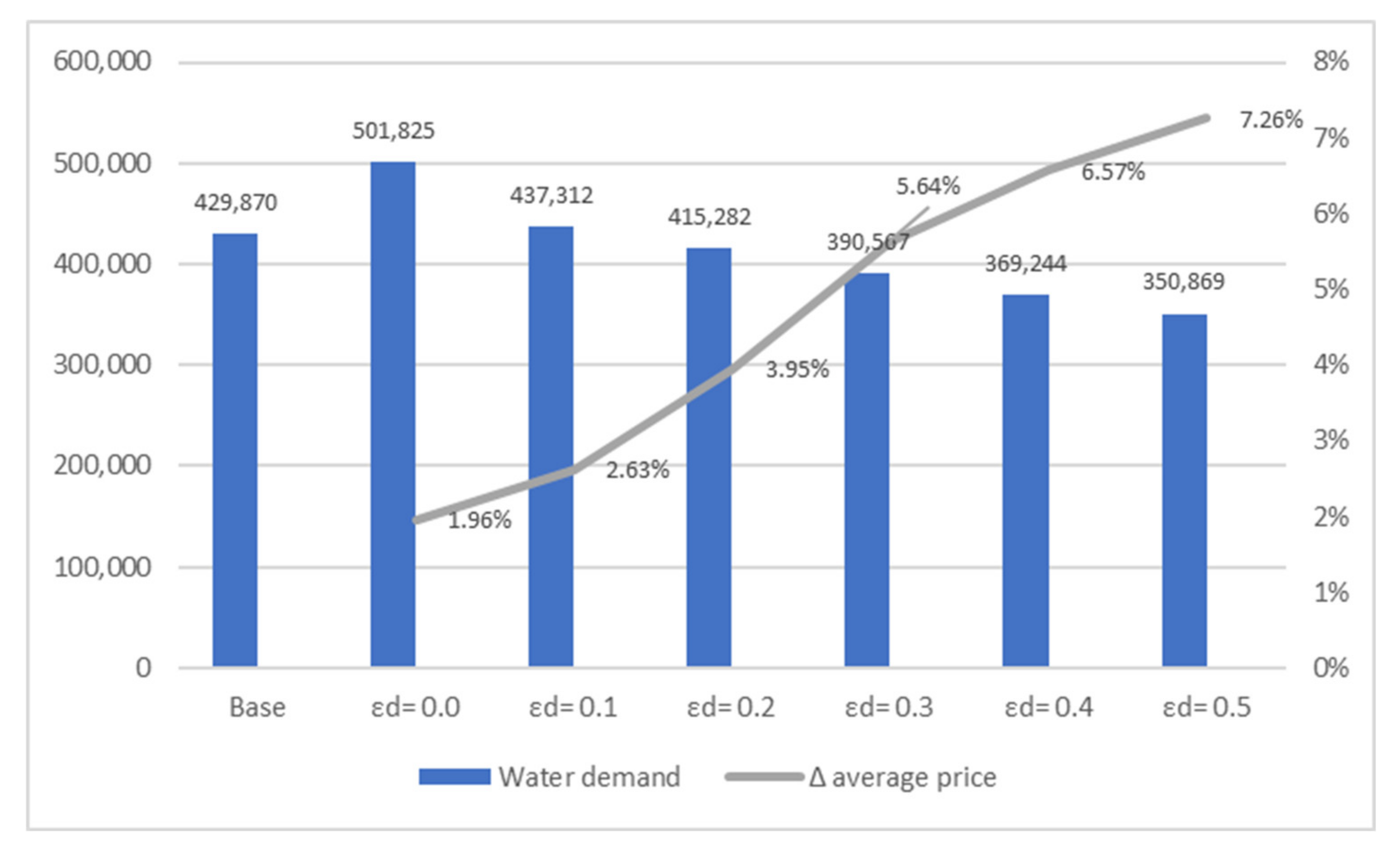
We did not consider introducing a sensitivity analysis due to the objective of our simulation model being precisely to implement numerous scenarios and show the changes in some parameters. In order to illustrate this goal, we introduce an example of how the water demand could change if we change one parameter (in this case, price elasticity). If we change price elasticity, water demand should be changed, due to the price increase or decrease. One of the advantages of the proposed model is that this new water demand would also change prices due to cost recovery conditions. Therefore, we can observe all the effects on prices and water demand if we change one of the parameters. The results of these changes can be seen in Figure 1.

In the model, cost recovery conditions increase water prices. If water demand decreases, water prices must increase to reach cost recovery goals. This is what we can see in Figure 1 when water demand decreases due to price elasticity. Considering that water demand is not influenced by prices (ε_p = 0.0), prices must be increased by an annual average of 1.96% in order to recover all water service costs, whereas water demand could reach more than 500,000 cubic meters. However, if water demand is significantly sensitive to price (ε_p = 0.5), water prices must be increased by an annual average of 7.26% due to a water demand reduction to 350,000 cubic meters.

5. Discussion

Most of the studies on water pricing often consider water demand as inelastic. This implies that there is no economic answer to pricing policies. Based on this approach, traditional water demand models take price as an external variable and use deterministic modeling methods, focused on population growth or fixed requirements.

Some experiences illustrate changes in water demand according to external incentives, as can be seen with awareness campaigns, even when water prices do not change. This appears to support the hypothesis of inelasticity.

However, recent experiences with water prices and water demand were analyzed by [25], which showed certain price sensitivity when this parameter was considered together with seasonal variability, household income, and the reality of each sector. This implies that water demand can be price-sensitive.

In the last few decades, hydro-economic models [31] emerged in order to link water demand, water availability, and water price. These models try to identify those economic values that impact water allocation, taking into account environmental water flows. These models can be split into two categories: simulation-based models and optimization-based models.

WaTaPro model is a simulation-based model that provides an answer to management decisions in terms of water demand and price levels. One outstanding feature of the WaTaPro model is price structure flexibility and cost-sharing. Most hydro-economic models do not provide flexible elements in pricing or cost-sharing mechanisms between different types of users [32]. Nevertheless, they can implement an economic value with respect to water flows and the environment. In fact, these models are designed to be used at the river basin level for all water uses, but WaTaPro is designed to be used at a local level for urban water use only, without considering environmental flows (only environmental cost). These are the reasons which justify the lack of a comparison between WaTaPro and other hydro-economic models.

6. Conclusions

In the last few years, there was a qualitative change of perspective for the approach in decision-making regarding the management of water services. Without abandoning the solutions envisaged on the supply side (increasing the level of availability of water resources and increasing water infrastructure), new measures were devised on the demand side for these services.

The tools available for service managers to implement measures in order to improve efficiency in the management of these services increased in recent years.

The use of simulation models for management development is at an inception stage with a long way still to go. The review in the present paper highlighted the usefulness of modeling and the potential benefits when using these tools to optimize the management of water services.

Water prices and demand models could also result in new water planning processes and the development of effective water price strategies to monitor water demand, in order to promote efficient investment and innovation in new and enhanced infrastructures.

There is huge potential for water saving when using these kinds of tools, which makes it possible to rapidly identify those useful elements as a valuable tool for strategic planning (water prices, cost recovery levels, contribution of the different water users, etc.), looking for alternatives to optimize the use of existing resources. Consequently, we can anticipate user behavior and prevent scarcity events.

However, as we can see in the case study, traditional water planning would increase water supply infrastructure in order to address rising water demand. However, if we consider all the facts affecting water demand, there is no increase in water consumption. Thus, we can consider this kind of tool as an investment leading to savings if we take into account the effective water demand.

We recognize that much work is still needed to address the issues related to water prices and water demand. In this vein, we need to improve the analysis of water price elasticity, as well as the matters of water use efficiency or income elasticity; hence, further research is required.