Assessing the Impacts of Climate Change and Land Use/Cover Change on Runoff Based on Improved Budyko Framework Models Considering Arbitrary Partition of the Impacts

Abstract

Various models based on Budyko framework, widely applied to quantify the impacts of climate change and land use/cover change (LUCC) on runoff, assumed a fixed partition used to distinguish the impacts. Several articles have applied a weighting factor describing arbitrary partitions for developing a total differential Budyko (TDB) model and a complementary Budyko (CB) model. This study introduces the weighting factor into a decomposition Budyko (DB) model and applies these three models to analyze runoff variation due to the impacts in the upper-midstream Heihe River basin. The Pettitt test is first applied to determine a change point of a time series expanded by the runoff coefficient. The cause for the change point is analyzed. Transition matrix is adopted to investigate factors of LUCC. Results suggest the consistency of the CB, TDB, and present DB models in estimating runoff variation due to the impacts. The existing DB model excluding the weighting factor overestimates the impact of climate change on runoff and underestimates the LUCC impact as compared with the present DB model. With two extreme values of the weighting factor, runoff decrease induced by LUCC falls in the range of 65.20%–66.42% predicted by the CB model, 65.01%–66.57% by the TDB model, and 64.83%–66.85% by the present DB model. The transition matrixes indicate the major factors of LUCC are climate warming in the upstream of the study area and cropping in the midstream. Our work provides researchers with a better understanding of runoff variation due to climate change and LUCC.

1. Introduction

Spatiotemporal variation of runoff has been an important component in hydrological cycle [1]. Climate change and land use/cover change (LUCC) are two major impacts on runoff [2]. Variation in temperature due to climate change causes the redistribution of precipitation to evapotranspiration and runoff [3]. Extreme hydrological events such as drought and flood influence runoff and intensify global water cycle [4,5,6]. On the other hand, LUCC such as deforestation and cultivation affects the regional water cycle and runoff [7]. A large amount of groundwater pumping for irrigation reduces runoff and increases evapotranspiration [8]. These therefore lead us to question how to differentiate and quantify the individual impacts of climate change and LUCC on runoff on reginal or global scale [9]. Exploring runoff variation due to the impacts helps researchers understand complex hydrological processes [10,11].

In recent decades, researchers have developed a variety of models for estimating runoff variation caused by climate change and LUCC in global catchments [12,13,14,15,16]. Most models depend on a natural runoff series without considering the LUCC impact and assume climate change and LUCC being decoupled. These models can be classified into three groups: empirical model, hydrological model, and water–energy balance model. The empirical model includes climate elasticity of runoff using nonparametric estimation [17] and statistical regression [18]. Parameters of the empirical model are estimated by linear regression, which requires long-term historical datasets [19]. The hydrological model [20] defines a physical explanation for each parameter but involves high uncertainty in parameter estimation [19,21]. The water–energy balance model, based on the Budyko framework [22] or the ecohydrological conceptual framework [23], has more physical structure than the empirical model and fewer parameters than the hydrological model. When coupled with trajectory analysis, the water–energy balance model is applicable in exploring the varying process of runoff and distinguishing the impacts of climate change and LUCC [21].

Variation in the Budyko curve in Figure 1 can account for the impacts of climate change and LUCC on runoff. Point A is regarded as a natural state without the impacts, but Point D is regarded as a state subjected to the impacts. The path from Point A to D is nonunique, leading to various partitions of the impacts. Path 1 (i.e., A–B–D) is, for example, regarded as the lower boundary and Path 2 (i.e., A–C–D) as the upper boundary. A vertical path between Paths 1 and 2 reflects the only LUCC impact. A segment on Path 1 or 2 accounts for the only impact of climate change. Most existing Budyko framework models, however, assume a fixed partition used to distinguish the impacts of climate change and LUCC on runoff. For releasing this assumption, a weighting factor was proposed to represent arbitrary paths from Point A to D for describing arbitrary partitions of the impacts [24,25]. The weighting factor was applied to develop two improved models of total differential Budyko (TDB) [22] and complementary Budyko (CB) [25]. The CB model was used to analyze runoff subject to the impacts in China [21,26]. As concluded, the weighting factor provides Budyko framework models with more flexibility of distinguishing the impacts.

A great deal of effort has been made on the developments of the TDB and CB models with the weighting factor [21,25,26]. What seems to be lacking, however, is to examine the consistency of multiple Budyko framework models based on the weighting factor accounting for arbitrary partitions of both climate change and LUCC impacts. In addition, a widely applied decomposition Budyko (DB) model has not considered the weighting factor [3].This study develops an improved DB model with the weighting factor and investigates the consistency of the DB, CB, and TDB models in assessing the impacts on runoff in the upper-midstream Heihe River basin during the study period of 1961–2014. The Mann–Kendall (MK) test and Sen’s slope are adopted for trend analysis. The Pettitt test is applied to determine a reasonable change point of runoff coefficient time series. The Mezentsev–Choudhury–Yang function [22,27,28] is used to define the Budyko curve. The effect of the weighting factor on model predictions is explored. In addition, the transition matrix is adopted to investigate factors of LUCC from 1980 to 2000. Our work provides implications for not only better understanding of runoff variation but also more reliability of Budyko framework models for attribution analysis.

2. Methodology

2.1. Trend Analysis

2.1.1. Mann–Kendall Test

Inspecting the trend of hydro-meteorological series is a critical task for exploring the relations between runoff Q and climate factors including precipitation P, and potential evapotranspiration E₀. Sen’s slope [29] and the non-parametric Mann–Kendall (MK) test [30,31] are used to identify temporal trends of P, E₀ and Q. Assume that each dataset of Q, P, and E₀, expressed as {x_i, x_i+1,…, x_n} with n being the total number, is independent and identically distributed. The test statistic S and the variance of S are defined as:

$$S={\displaystyle \sum }_{i=1}^{n-1}{\displaystyle \sum }_{j=i+1}^n\mathrm{sgn}(x_j-x_i)$$

(1)

$$\mathrm{sgn}(\mathsf{\theta })=\{\begin{array}{ll}1& \theta >0\\ 0& \theta =0\\ -1& \theta <0\end{array}$$

(2)

$$Var(S)=n(n-1)(2n+5)/18$$

(3)

The standardized test statistic Z for the standard normal distribution is calculated by:

$$Z=\frac{1}{\sqrt{var(S)}}\{\begin{array}{ll}s-1& S>0\\ 0& S=0\\ s+1& S<0\end{array}$$

(4)

The significance level is set to 10%. With the significance level, the null hypothesis of no trend was rejected if |Z| > 1.645.

2.1.2. Sen’s Slope

The slope β for a time series {x_i, x_i+1,…, x_n} proposed by Sen [29] is expressed as:

$$\beta =\mathrm{median}\left(\frac{x_i-x_j}{i-j}\right),\forall j<i,1\le j<i\le n$$

(5)

A positive value of β indicates an increase, while a negative value indicates a decrease.

2.2. Pettitt Test for Determination of Change Point

A change point, dividing the study period into baseline and variation periods, needs to be determined before assessing the impact of LUCC on runoff. The baseline period before the change point assumes no LUCC impact. The non-parametric Pettitt test is used to detect a change point of a time series [32]. Qiu et al. [33] revealed the Pettitt test to a time series of P or Q for the Heihe river basin did not give a unique and significant change point. For determining a change point, this study therefore applies the Pettitt test to runoff coefficient defined as σ = Q/P accounting for the relation between P and Q.

Considering a time series {x_i, x_i+1,…, x_N} with N being the total number, the Pettitt test uses the Mann-Whitney statistic U_t,N that verifies if two subseries {x₁, …, x_t} and {x_t+1, …, x_N} result from the same population. The test statistic U_t,N is defined as:

$$U_{t,N}={\displaystyle \sum }_{i=1}^t{\displaystyle \sum }_{j=t+1}^N\mathrm{sgn}(x_i-x_j) \mathrm{for} t=1,\dots ,N-1$$

(6)

$$\mathrm{sgn}(\mathsf{\theta })=\{\begin{array}{cc}1& \theta >0\\ 0& \theta =0\\ -1& \theta <0\end{array}$$

(7)

A most significant change point will be determined when the value of |U_t,N| is a maximum, i.e., $K_{t,N}=\max (\left|U_{t,N}\right|)$. The significance level associated with K_t,N is expressed as:

$$\rho \cong 2\exp (\frac{-6K_{t,N}^2}{N^3+N^2})$$

(8)

When $\rho <5\%$, the null hypothesis is rejected.

2.3. Budyko Framework

The Budyko [34,35] framework is based on the physical principles proposed by Schreiber [36] and Ol’Dekop [37]. The annual average actual evapotranspiration is dominated by the balance between the water supply of the atmosphere and the demand of atmospheric evaporation. A number of articles have presented various functions based on the Budyko framework for describing the relation between the long-term average of E/P and the dryness index of E₀/P. The commonly used Mezentsev-Choudhury-Yang function is expressed as:

$$\frac{E}{P}=f(P,E_0,\omega )={(1+{(\frac{E_0}{P})}^{-\omega })}^{-1/\omega }$$

(9)

where ω is a parameter reflecting catchment characteristic. By applying Equation (9) and ignoring change in the long-term storage, the runoff Q can be expressed as:

$$Q=P-E=P-f(P,E_0,\omega )P$$

(10)

The ω can thus be obtained by Equation (10) with annual values of observed P, E₀, and Q. The change in observed runoff $\Delta Q_{obs}$ is the difference in the mean annual runoffs $Q_b$ for baseline period and $Q_v$ for variation period, written as:

$$\Delta Q_{obs}=Q_v-Q_b$$

(11)

The change in estimated runoff $\Delta Q_{est}$ contains two components associated with the impacts of climate change $\Delta Q_{clim}$ and LUCC $\Delta Q_{lucc}$, expressed as:

$$\Delta Q_{est}=\Delta Q_{clim}+\Delta Q_{lucc}$$

(12)

The contribution rates of climate change ${\eta }_{clim}$ and LUCC ${\eta }_{lucc}$ can be respectively written as [38]:

$${\eta }_{clim}=\frac{\Delta Q_{clim}}{\left|\Delta Q_{clim}\right|+\left|\Delta Q_{lucc}\right|}\times 100\%$$

(13)

$${\eta }_{lucc}=\frac{\Delta Q_{lucc}}{\left|\Delta Q_{clim}\right|+\left|\Delta Q_{lucc}\right|}\times 100\%$$

(14)

Three models of CB, TDB, and DB are discussed in the following subsections.

2.3.1. Complementary Budyko (CB) Model

The CB model starts from complementary relationship of the elasticity coefficients associated with precipitation and potential evapotranspiration, expressed as [24]:

$$\frac{\partial Q/Q}{\partial P/P}+\frac{\partial Q/Q}{\partial E_0/E_0}=1$$

(15)

Equation (15) reduces to:

$$Q=P\frac{\partial Q}{\partial P}+E_0\frac{\partial Q}{\partial E_0}$$

(16)

The change of runoff Q in Equation (16) is written as [25]:

$$dQ=(\frac{\partial Q}{\partial P})dP+(\frac{\partial Q}{\partial E_0})d{E}_0+Pd(\frac{\partial Q}{\partial P})+E_{0}d(\frac{\partial Q}{\partial E_0})$$

(17)

The weighting factor α is used to represent different paths from Point A to Point D in Figure 1 [21]. For Path 1 with α = 0, Point A to B reflects a fixed ratio of $E_0/P$ and a varying ω, indicating $E_0$ and P are assumed constant in baseline period and the catchment characteristic parameter is the only variable accounting for the impact of LUCC on runoff from baseline period to variation period. The path from Point B to D indicates the only impact of climate change on runoff with a fixed catchment characteristic parameter of variation period (i.e., ${\omega }_v$) with subscript v being variation period. For Path 2 with α = 1, the segment from Point A to C accounts for the only impact of climate change on runoff from baseline period to variation period with a fixed catchment characteristic parameter of baseline period (i.e., ${\omega }_b$) with subscript b being baseline period. The vertical descent from Point C to D reflects the only impact of LUCC due to the change of the catchment characteristic parameter (from ${\omega }_b$ to ${\omega }_v$). For an arbitrary path between Paths 1 and 2, Equation (17) with the weighting factor α becomes:

$$\begin{gathered} \Delta Q_{est}=\alpha \left(\frac{\partial Q_b}{\partial P_b}\Delta P+\frac{\partial Q_b}{\partial E_{0,b}}\Delta E_0\right)+(1-\alpha )\left(\frac{\partial Q_v}{\partial P_v}\Delta P+\frac{\partial Q_v}{\partial E_{0,v}}\Delta E_0\right) \\ +\alpha \left(P_b\Delta \frac{\partial Q}{\partial P}+E_{0,b}\Delta \frac{\partial Q}{\partial E_0}\right)+(1-\alpha )\left(P_v\Delta \frac{\partial Q}{\partial P}+E_{0,v}\Delta \frac{\partial Q}{\partial E_0}\right) \end{gathered}$$

(18)

The first two terms on the right-hand side stand for the impact of climate change, and the rest terms for the impact of LUCC.

2.3.2. Total Differential Budyko (TDB) Model

The TDB model with a first-order approximation to $Q=P-f(P,E_0,\omega )P$ can be written as [22]:

$$dQ=\left(\frac{\partial Q}{\partial P}\right)dP+\left(\frac{\partial Q}{\partial E_0}\right)d{E}_0+\left(\frac{\partial Q}{\partial \omega }\right)d\omega$$

(19)

Similar to the derivation of Equation (18), the change of runoff for arbitrary paths represented by weighting factor α can be expressed as [25]:

$$\begin{gathered} \Delta Q_{est}\approx \alpha \left(\frac{\partial Q_b}{\partial P_b}\Delta P+\frac{\partial Q_b}{\partial E_{0,b}}\Delta E_0\right)+(1-\alpha )\left(\frac{\partial Q_v}{\partial P_v}\Delta P+\frac{\partial Q_v}{\partial E_{0,v}}\Delta E_0\right)+\alpha \frac{\partial Q_b}{\partial {\omega }_b}\Delta \omega \\ +(1-\alpha )\frac{\partial Q_v}{\partial {\omega }_v}\Delta \omega \end{gathered}$$

(20)

The first two terms on the right-hand side of Equation (20) are identical to those of Equation (18). The TDB model gives error in prediction because of applying the first-order approximation. This will be discussed in Section 4.2.

2.3.3. The Present Decomposition Budyko (DB) Model

Existing DB model is a graphic model based on Budyko curve represented by Path 2 with α = 1 (i.e., A–C–D) in Figure 1 [3]. With Path 2, the impacts of climate change and LUCC on runoff can be written as:

$$\Delta Q_{clim}=P_v(1-E_v^{\prime })-P_b(1-E_b)$$

(21)

$$\Delta Q_{lucc}=P_v(E_v^{\prime }-E_v)$$

(22)

where $E_b=f(P_b,E_{0,b},{\omega }_b)$, $E_v=f(P_v,E_{0,v},{\omega }_v)$, and $E_v^{\prime }=f(P_v,E_{0,v},{\omega }_b)$. Due to the uncertainty of path [25], Path 1 with α = 0 (i.e., A–B–D) is also a possible way to assess runoff variation due to the impacts, expressed as:

$$\Delta Q_{clim}=P_v(1-E_v)-P_b(1-E_b^{\prime })$$

(23)

$$\Delta Q_{lucc}=P_b(E_b-E_b^{\prime })$$

(24)

where $E_b^{\prime }=f(P_b,E_{0,b},{\omega }_v)$. Based on Equations (21)–(24), the present DB model with the weighting factor α accounting for an arbitrary path between Paths 1 and 2 can be expressed as:

$$\begin{gathered} \Delta Q_{est}=\alpha (P_v(1-E_v^{\prime })-P_b(1-E_b))+(1-\alpha )(P_v(1-E_v)-P_b(1-E_b^{\prime })) \\ +\alpha (P_v(E_v^{\prime }-E_v))+(1-\alpha )(P_b(E_b-E_b^{\prime })) \end{gathered}$$

(25)

Table 1. The expressions of climate change impact $\Delta Q_{clim}$ and LUCC impact $\Delta Q_{lucc}$ for the three models.

Models	$\Delta {\mathit{Q}}_{\mathit{c}\mathit{l}\mathit{i}\mathit{m}}$	$\Delta {\mathit{Q}}_{\mathit{l}\mathit{u}\mathit{c}\mathit{c}}$
CB	$\alpha \left(\frac{\partial Q_b}{\partial P_b}\Delta P+\frac{\partial Q_b}{\partial E_{0,b}}\Delta E_0\right)+(1-\alpha )\left(\frac{\partial Q_v}{\partial P_v}\Delta P+\frac{\partial Q_v}{\partial E_{0,v}}\Delta E_0\right)$	$\alpha \left(P_b\Delta \frac{\partial Q}{\partial P}+E_{0,b}\Delta \frac{\partial Q}{\partial E_0}\right)+(1-\alpha )\left(P_v\Delta \frac{\partial Q}{\partial P}+E_{0,v}\Delta \frac{\partial Q}{\partial E_0}\right)$
TDB	$\alpha \left(\frac{\partial Q_b}{\partial P_b}\Delta P+\frac{\partial Q_b}{\partial E_{0,b}}\Delta E_0\right)+(1-\alpha )\left(\frac{\partial Q_v}{\partial P_v}\Delta P+\frac{\partial Q_v}{\partial E_{0,v}}\Delta E_0\right)$	$\alpha \frac{\partial Q_b}{\partial {\omega }_b}\Delta \omega +(1-\alpha )\frac{\partial Q_v}{\partial {\omega }_v}\Delta \omega$
The present DB	$\alpha (P_v(1-E_v^{\prime })-P_b(1-E_b))+(1-\alpha )(P_v(1-E_v)-P_b(1-E_b^{\prime }))$	$\alpha (P_v(E_v^{\prime }-E_v))+(1-\alpha )(P_b(E_b-E_b^{\prime }))$

shows the expressions of $\Delta Q_{clim}$ and $\Delta Q_{lucc}$ for the CB, TDB, and present DB models.

2.4. Transition Matrix of Land Use

Transition matrix of land use accounts for change of land use during different periods. The types of land use are classified into: crop-lands, forest, grassland, water bodies, snow and ice, urban and built-up, and barren in this study. The transition matrix of land use is obtained by using the Spatial Analyst Tools of ArcGIS function. One can refer to the study by Liu et al. [39] for detailed description of transition matrix.

3. Study Area and Datasets

The Heihe River, the second largest inland river in the south Qilian Mountain of northwestern China, suffers from serious water scarcity. The river generally flows northwards towards Mongolia. The main river channel (98°–101° E, 38°–42° N) is 821 km long. The total catchment area is 14.31 × 10⁵ km². Two main hydrological stations, Yingluoxia and Zhengyixia, divide the Heihe River basin into three sub-basins (upper, middle, and downstream). The upper and middle Heihe River basins, which contain alpine ice-snow and permafrost, mountainous forest zones, and a plain oasis agriculture zone, are selected as the study area (Figure 2). The water sources of the upstream are mainly precipitation and glacier melt water. The midstream basin is an important commodity grain-producing area in a representative piedmont valley plain oasis.

Daily meteorological data at five meteorological stations in the study area were downloaded from the China Meteorological Data Sharing Service System (http://data.cma.cn/). Measurement of monthly runoff at the Zhengyixia hydrological station was collected from the Gansu Provincial Hydrological Bureau. The hydro-meteorological datasets for the upper and middle reaches spanned the period of 1961–2014. The daily potential evapotranspiration was estimated using the Penman-Monteith equation as suggested by Food and Agriculture Organization of the United Nations (FAO) [40]. The data of five meteorological stations with a resolution of $1 \mathrm{km}\times 1 \mathrm{km}$ were spatially averaged by the Inverse Distance Weighted (IDW) method. The daily precipitation and potential evapotranspiration and monthly runoff were aggregated to obtain the individual time series expanded by 54 annual totals. In addition to the meteorological data, remotely sensed land use maps of 1980 and 2000 with a resolution of $1 \mathrm{km}\times 1 \mathrm{km}$ were provided by the Resource and Environment Data Cloud Platform of the Chinese Academy of Sciences (http://www.resdc.cn/) and adopted to analyze the change in land use and cover in the study area.

4. Results and Discussion

4.1. Trend Analysis of Hydro-Meteorological Series and Determination of Change Point

The trend analysis of hydro-meteorological series is conducted by applying the MK test and Sen’s slope for better understanding runoff process during the study period of 1961–2014. The results of trend analysis are shown in

Table 2. Summary of trend analysis for hydro-meteorological series.

Parameter	P	E0	Q
β (mm/yr)	0.8	0.25	−0.01
Z	2.40 ***	0.67	−0.13
Annual Mean (mm/yr)	251.09	946.49	28.47

Note: *** denotes the confidence level of 10%.

. The mean annual runoff (i.e., 28.47 mm/yr) is much smaller than the mean annual precipitation (i.e., 251.09 mm/yr) or potential evapotranspiration (i.e., 946.49 mm/yr). The trends of all meteorological factors were increasing. In contrast, a slight downward trend is detected for Q. The results of β > 0 or Z > 0 for P and β < 0 or Z < 0 for Q indicate a negative correlation between P and Q, which contradicts the linear positive correlation in the natural state. This may be attributed to the fact that irrigation and farming increased evapotranspiration and reduced runoff in the midstream of the Heihe River basin, important agricultural area [3]. It can be reasoned that the runoff variation is therefore related to both climate change and LUCC.

The change point divides the study period of 1961–2014 into a baseline period and a variation period according to the Pettitt test [32]. Figure 3 shows temporal distributions of U_t,N from the Pettitt test used to annual time series of precipitation P, runoff Q and runoff coefficient σ = Q/P. The unremarkable peak at 2001 for P as well as the peaks at 1983 and 2002 for Q are below the significance level of 10%, failing to pass the significance test. The only peak at 1984 for σ = 0.14, passing the significance test of 5%, can be regarded as a change point that reflects a significant change in the relation of runoff and precipitation. With the change point of 1984, the available data can be divided into the baseline period of 1961–1984 and the variation period of 1985–2014.

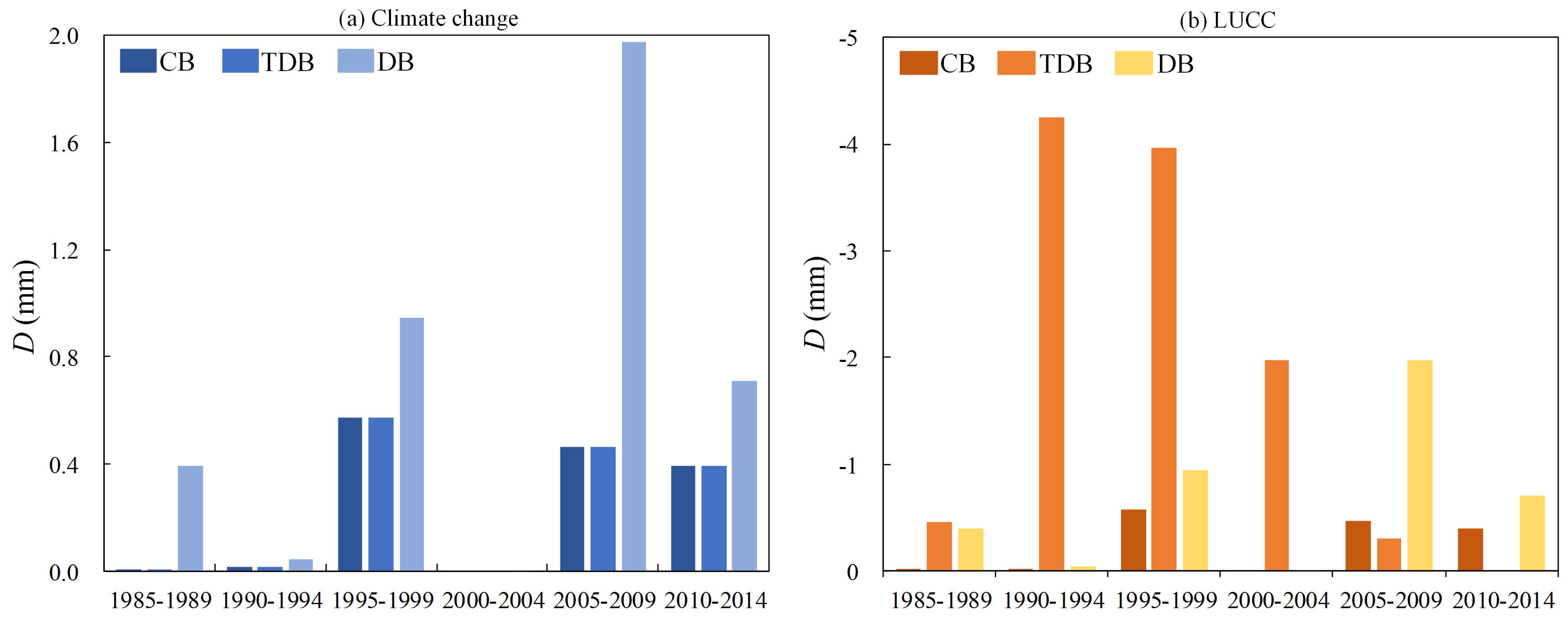
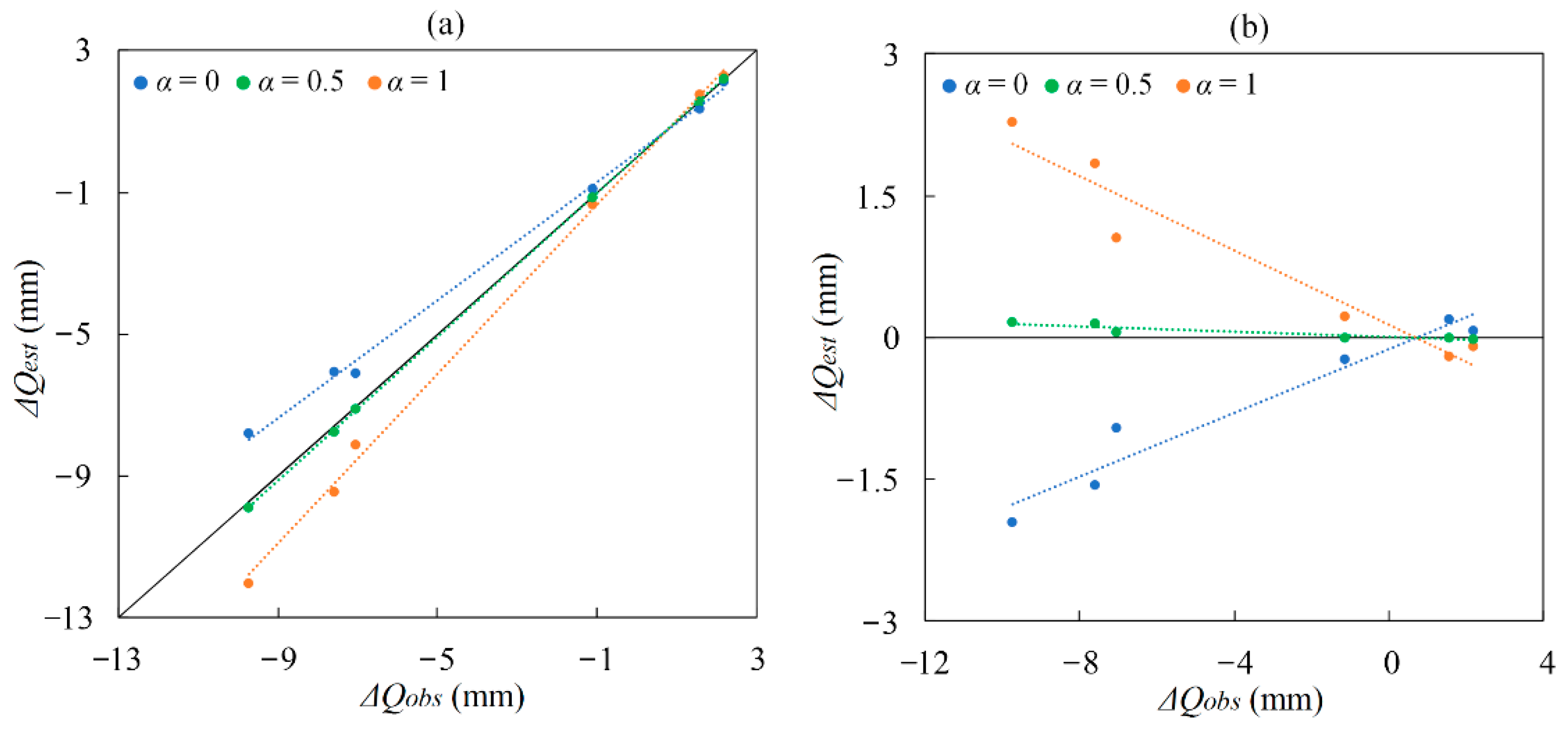
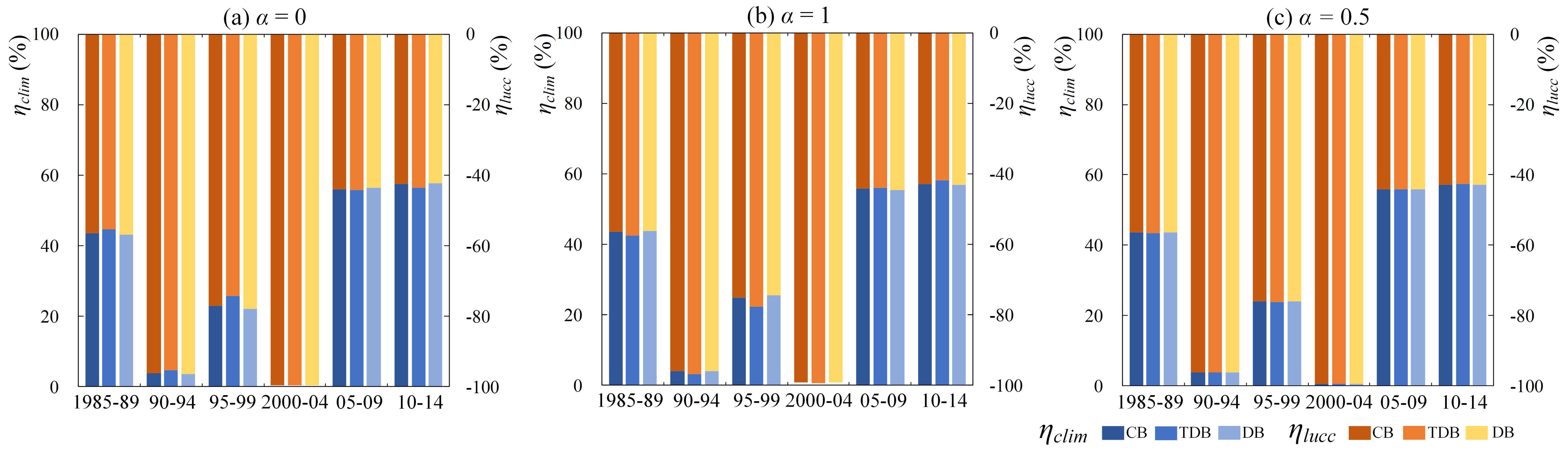
4.2. The Impacts of Climate Change and LUCC on Runoff Based on the Budyko Framework Models

For better understanding the behavior of runoff change, the variation period of 1985–2014 is divided into six sub-variation periods of five years. Figure 4 illustrates the straight paths from the baseline period of 1961–1984 to the six sub-variation periods based on the Budyko framework. Each path moves from the baseline period to the upper left, indicating a greater increase in P than that in E₀; therefore, the climate therein became moister. The upper component of each path represents runoff increase due to climate change, and the leftward component accounts for runoff decrease caused by LUCC.

Table 3. The impacts of climate change and LUCC as well as contribution rates calculated by the complementary Budyko (CB), total differential Budyko (TDB) and present decomposition Budyko (DB) models for three cases of α = 0 for the lower boundary, α = 1 for the upper boundary, and α = 0.5 in between.

	$\Delta {\mathit{Q}}_{\mathit{c}\mathit{l}\mathit{i}\mathit{m}}(\mathbf{mm})$			$\Delta {\mathit{Q}}_{\mathit{l}\mathit{u}\mathit{c}\mathit{c}}(\mathbf{mm})$			${\mathit{\eta }}_{\mathit{c}\mathit{l}\mathit{i}\mathit{m}}(\%)$			${\mathit{\eta }}_{\mathit{l}\mathit{u}\mathit{c}\mathit{c}}(\%)$
	CB	TDB	DB	CB	TDB	DB	CB	TDB	DB	CB	TDB	DB
The lower boundary (α = 0)	3.71	3.71	3.57	−7.34	−6.90	−7.20	33.58	34.99	33.15	−66.42	−65.01	−66.85
The upper boundary (α = 1)	4.15	4.15	4.30	−7.78	−8.27	−7.93	34.80	33.43	35.17	−65.20	−66.57	−64.83
In between (α = 0.5)	3.93	3.93	3.94	−7.56	−7.59	−7.57	34.22	34.15	34.22	−65.78	−65.85	−65.78

displays the impacts of climate change and LUCC on runoff (i.e., $\Delta Q_{clim}$ and $\Delta Q_{lucc}$) as well as the contribution rates (i.e., ${\eta }_{clim}$ and ${\eta }_{lucc}$) estimated by the CB, TDB, and the present DB models considering the causes of α = 0 for the lower boundary of Path 1, α = 1 for the upper boundary of Path 2, and α = 0.5 in between during the variation period of 1985–2014. A reasonable range between two estimates for the cases of α = 0 and α = 1 can be seen. The estimates for the case of α = 0.5 fall in their own ranges. Existing DB model, a special case of the present DB model with α = 1, overestimates ${\eta }_{clim}$ and underestimates $\left|{\eta }_{lucc}\right|$ as compared with those predicted by the present DB model with α = 0.5. Reasonable ranges of 33.15%–35.17% for ${\eta }_{clim}$ and 64.83%–66.85% for $\left|{\eta }_{lucc}\right|$ are obtained using the present DB model. It is worth noting that the three models give close values of ${\eta }_{lucc}$ for the case of α = 0.5, indicating LUCC is the main cause for runoff decrease in the ranges of 65.20%–66.42% predicted by the CB model, 65.01%–66.57% by the TDB model and 64.83%–66.85% by the present DB model. Qiu et al. [33] reported $\left|{\eta }_{lucc}\right|=53\%$ predicted by the sensitivity model based on the Budyko framework. Our three models predict greater values of $\left|{\eta }_{lucc}\right|$ than theirs. The difference may result from the following reasons. Their model applies the Zhang et al. [12] function with the period of 1964–2006 while our models are based on the Yang et al. [22] function with the period of 1961–2014. In addition, our models consider the weighting factor α, but their model does not.

Define difference D in the value of either $\Delta Q_{clim}$ or $\Delta Q_{lucc}$ between Paths 1 for α = 0 and Path 2 for α = 1. Although the three models give close ranges of $\Delta Q_{clim}$ for the variation period of 1985–2014 in Table 3, the present DB model predicts a greater D than the others for each sub-variation period in Figure 5a. This may come from the fact that the present DB model, a graphical model, relies on two variables of ratio $E_0/P$ and ω using Equation (9) while the others depend on three variables of $E_0$, P, and ω using Equations (18) and (20). It is worth noting that the CB and TDB models give exact the same D in Figure 5a because of the identical expression in Table 1 for $\Delta Q_{clim}$. The TDB model, however, gives inaccurate results of much greater D for $\Delta Q_{lucc}$ than the CB model for the first four sub-variation periods in Figure 5b because the first-order approximation of the TDB model causes a residual runoff change $\Delta Q_{res}$, defined as an observed runoff change $\Delta Q_{obs}$ minus an estimated one $\Delta Q_{est}$. Figure 6 shows the relations of $\Delta Q_{est}$ and $\Delta Q_{obs}$ in panel (a) as well as $\Delta Q_{res}$ and $\Delta Q_{obs}$ in panel (b) for the six sub-variation periods estimated by the TDB model with α = 0 for the lower boundary, α = 1 for the upper boundary, and α = 0.5 in between. When α = 0, $\Delta Q_{res}$ is of significantly positive relation with $\Delta Q_{obs}$. The $\left|\Delta Q_{est}\right|$ is underestimated as compared with $\left|\Delta Q_{obs}\right|$. When α = 1, there is a negative correlation between $\Delta Q_{res}$ and $\Delta Q_{obs}$, leading to an overestimate of $\left|\Delta Q_{est}\right|$. Our results for the cases of α = 0 and 1 accord with the findings of Zhou et al. [25] and Wang et al. [26] that $\left|\Delta Q_{est}\right|$ by the TDB model was significantly underestimated for α = 0 and overestimated for α = 1 compared with $\left|\Delta Q_{obs}\right|$. When α = 0.5, $\Delta Q_{res}$ approaches zero and can be ignored, indicating the TDB model gives close values of $\Delta Q_{clim}$, $\Delta Q_{lucc}$, ${\eta }_{clim}$, and ${\eta }_{lucc}$ to the others in Table 3. Error in $\Delta Q_{est}$ by the TDB model, in other words, becomes minor for α approaching 0.5.

Figure 7 shows the contribution rates ${\eta }_{clim}$ and ${\eta }_{lucc}$ for six sub-variation periods predicted by the CB, TDB, and the present DB models with α = 0 for the lower boundary, α = 1 for the upper boundary, and α = 0.5 in between. The three models agree to ${\eta }_{clim}$ and ${\eta }_{lucc}$ with minor error for each sub-variation period. The magnitude of $\left|{\eta }_{lucc}\right|$ is the largest in the sub-variation period of 2000–2004 for each model and each α and then decreases after the that period. This may be because China has experienced a striking economic boom with reform and opening-up policy since 1980 [38]. Population growth and economic development increased water withdrawal and utilization, resulting in a decrease in runoff. Since then, ${\eta }_{clim}$ generally increased and exceeded 50%, indicating that climate change impact dominates runoff change in the last two sub-variation periods. In addition, Figure 7 displays dramatically temporal variability of ${\eta }_{clim}$ and ${\eta }_{lucc}$ during the entire period except the last sub-variation period, which is similar to the finding of Wang et al. [26].

4.3. Factors of LUCC

A variety of studies have considered the change in ω (i.e., Δω) related to human activities. Roderick and Farquhar [41], however, revealed that Δω is linked to rainfall intensity of climate factor. Jiang et al. [42] estimated Δω according to the factors of temperature, potential evapotranspiration and irrigated area and found errors in Δω caused by assuming Δω due to human activities. Since LUCC is the dominant cause of runoff change in the study area as concluded in Section 4.2, this section applies the transition matrix of land use types for analyzing factors of LUCC.

Table 4. The transition matrixes of seven land use types for the upstream and midstream of the Heihe River basins from 1980 to 2000 (unit: km²).

Land Use Types		Upstream/Midstream (2000)
		Crop-Lands	Forest	Grass-Land	Water Bodies	Snow and Ice	Urban and Built-Up	Barren
Upstream (1980)	Croplands	27	0	0	0	0	0	0
	Forest	0	2107	0	0	0	0	0
	Grassland	0	0	4997	0	0	0	0
	Water Bodies	0	0	0	175	0	0	0
	Snow and Ice	0	2	51	0	76	0	99
	Urban and Built-Up	0	0	0	0	0	10	0
	Barren	0	0	0	0	0	0	2413
Midstream (1980)	Croplands	3483	0	32	5	0	11	1
	Forest	6	2427	16	0	0	0	9
	Grassland	226	5	7298	0	0	5	30
	Water Bodies	31	0	4	498	0	0	0
	Snow and Ice	0	0	0	0	57	0	11
	Urban and Built-Up	0	0	0	0	0	309	0
	Barren	46	0	3	1	0	4	10,511

shows the transition matrixes for describing LUCC from 1980 to 2000 in the upstream and midstream of the Heihe River basin. Grassland and barren occupied most of the area. In the upstream, the type of snow and ice was mainly converted into grassland and barren. Hao and Zong [43] also revealed this snow–ice area shrunk by half and turned into grassland and barren because of climate warming since 1980s. The reduction of the snow–ice area due to rising temperature and the spatiotemporal change of precipitation significantly affected runoff. In the midstream, four types (i.e., forest, grassland, water bodies, and barren) are converted into cropland, because the midstream is an important grain-producing area. More than eighty percent of water withdrawal was used to irrigate farmland, which is regarded as the main human activities in the midstream [44]. The increase in cropland indicates cropping is the major human activity resulting in LUCC. This result is consistent with the studies [45,46]. The grassland area also increased from the areas of the other types as a result of the Grain for Green Program. As concluded, the transition matrixes suggest the main factors of LUCC are climate warming in upstream and cropping in midstream, reflecting the impacts of not only climate change but also human activities. This result accords with the finding of Luo et al. [47] that runoff variation in the upstream is caused by climate change and in the midstream by LUCC.

5. Conclusions

To conclude, this study is preliminary research on the impacts of climate change and LUCC on runoff in the upper-midstream Heihe River basin, but its relevance to Budyko framework models can be seen. A major finding is the consistency of the CB, TDB, and present DB models in predicting runoff variation due to the impacts for the study area. The results indicate the weighting factor α is applicable in providing a flexible and reasonable partition of both impacts on runoff. It can be reasoned that the impacts simultaneously induce runoff variation in the study area. Existing DB model excluding α gives an overestimated climate change impact on runoff and underestimated LUCC impact in comparison with the present DB model. In addition, error due to first-order approximation used to develop the TDB model becomes minor when α = 0.5. Furthermore, the extreme values of α = 0 and 1 can be used to quantify uncertainty of the impacts in providing those ranges in Table 3.

Our findings are consistent with those of the articles discussed above. With respect to the weighting factor α, our findings confirm those of Zhou et al. [25] and Wang et al. [26] although there are some differences regarding other aspects of the studies. These results lend some credence to the hypothesis that estimated runoff change $\left|\Delta Q_{est}\right|$ is underestimated by the TDB model for α = 0 and overestimates it for α = 1 as compared with observed runoff change $\left|\Delta Q_{obs}\right|$. The discrepancy between $\Delta Q_{est}$ and $\Delta Q_{obs}$ results from the first-order approximation but becomes minor for α = 0.5. In addition, our finding is similar to that of Wang et al. [26]. The result indicates dramatically temporal variability of the contribution rates of climate change and LUCC to runoff during 1985–2014 because China has encountered striking economic boom since 1980. Moreover, our study agrees with Luo et al. [47]. The transition matrixes reveal the major factors of LUCC are climate warming in the upstream of the Heihe River basin and cropping in midstream. This finding is indicative of the fact that the reasons of inducing runoff variation are due to both climate change and LUCC in the study area.

This study has demonstrated the weighting factor is needed and should be stressed in assessing the impacts of climate change and LUCC on runoff. It follows that the use of multiple Budyko framework models are also needed for achieving reliability of model predictions. Our work provides researchers with a better understanding of runoff variation due to the impacts for semi-arid regions. However, whether this will also apply to humid regions of the world cannot be determined on the basis of this study. Further research is therefore warranted in exploring runoff variation induced by the impacts in humid regions using Budyko framework models with the weighting factor.

References

1. Yang, T.; Wang, C.; Chen, Y.; Chen, X.; Yu, Z. Climate change and water storage variability over an arid endorheic region. J. Hydrol. 2015, 529, 330–339. [Google Scholar] [CrossRef]
2. Tuladhar, D.; Dewan, A.; Kuhn, M.; Corner, R.J. The Influence of Rainfall and Land Use/Land Cover Changes on River Discharge Variability in the Mountainous Catchment of the Bagmati River. Water 2019, 11, 2444. [Google Scholar] [CrossRef] [Green Version]
3. Wang, D.; Hejazi, M. Quantifying the relative contribution of the climate and direct human impacts on mean annual streamflow in the contiguous United States. Water Resour. Res. 2011, 47. [Google Scholar] [CrossRef] [Green Version]
4. Ma, X.F.; Yan, W.; Zhao, C.Y.; Kundzewicz, Z.W. Snow-Cover Area and Runoff Variation under Climate Change in the West Kunlun Mountains. Water 2019, 11, 2246. [Google Scholar] [CrossRef] [Green Version]
5. Allan, R.P.; Soden, B.J. Atmospheric warming and the amplification of precipitation extremes. Science 2008, 321, 1481–1484. [Google Scholar] [CrossRef] [PubMed] [Green Version]
6. Shi, P.; Yang, T.; Xu, C.-Y.; Gourley, J.J.; Shao, Q.; Li, Z.; Wang, X.; Zhou, X.D.; Li, S. How do the multiple large-scale climate oscillations trigger extreme precipitation? Glob. Planet. Chang. 2017, 157, 48–58. [Google Scholar] [CrossRef]
7. Wang, X.J.; Zhang, P.F.; Liu, L.L.; Li, D.D.; Wang, Y.P. Effects of Human Activities on Hydrological Components in the Yiluo River Basin in Middle Yellow River. Water 2019, 11, 689. [Google Scholar] [CrossRef] [Green Version]
8. Hu, Y.; Moiwo, J.P.; Yang, Y.; Han, S.; Yang, Y. Agricultural water-saving and sustainable groundwater management in shijiazhuang irrigation district, north china plain. J. Hydrol. 2010, 393, 219–232. [Google Scholar] [CrossRef]
9. Marie, J.; Jacques, S.; Sauchyn, D.J.; Zhao, Y. Northern rocky mountain streamflow records: Global warming trends, human impacts or natural variability? Geophys. Res. Lett. 2010, 37, 53–67. [Google Scholar] [CrossRef] [Green Version]
10. Chang, Q.R.; Zhang, C.; Zhang, S.; Li, B.Q. Streamflow and Sediment Declines in a Loess Hill and Gully Landform Basin Due to Climate Variability and Anthropogenic Activities. Water 2019, 11, 2352. [Google Scholar] [CrossRef] [Green Version]
11. Yang, S.; Kang, T.T.; Bu, J.Y.; Chen, J.H.; Gao, Y.C. Evaluating the Impacts of Climate Change and Vegetation Restoration on the Hydrological Cycle over the Loess Plateau, China. Water 2019, 11, 2241. [Google Scholar] [CrossRef] [Green Version]
12. Zhang, L.; Zhao, F.; Chen, Y.; Dixon, R.N.M. Estimating effects of plantation expansion and climate variability on streamflow for catchments in Australia. Water Resour. Res. 2011, 47. [Google Scholar] [CrossRef]
13. Li, H.; Zhang, Y.; Vaze, J.; Wang, B. Separating effects of vegetation change and climate variability using hydrological modelling and sensitivity-based approaches. J. Hydrol. 2012, 420–421, 403–418. [Google Scholar] [CrossRef]
14. Wang, W.; Shao, Q.; Yang, T.; Peng, S.; Xing, W.; Sun, F.; Luo, Y. Quantitative assessment of the impact of climate variability and human activities on runoff changes: A case study in four catchments of the Haihe River basin, China. Hydrol. Process. 2012, 27, 1158–1174. [Google Scholar] [CrossRef]
15. Dey, P.; Mishra, A. Separating the impacts of climate change and human activities on streamflow: A review of methodologies and critical assumptions. J. Hydrol. 2017, 548, 278–290. [Google Scholar] [CrossRef]
16. Wu, J.; Miao, C.; Zhang, X.; Yang, T.; Duan, Q. Detecting the quantitative hydrological response to changes in climate and human activities. Sci. Total. Environ. 2017, 586, 328–337. [Google Scholar] [CrossRef]
17. Sankarasubramanian, A.; Vogel, R.M.; Limbrunner, J.F. Climate elasticity of streamflow in the United States. Water Resour. Res. 2001, 37, 1771–1781. [Google Scholar] [CrossRef]
18. Vogel, R.M.; Wilson, I.; Daly, C. Regional regression models of annual streamflow for the United States. J. Irrig. Drain. Eng. 1999, 125, 148–157. [Google Scholar] [CrossRef]
19. Xu, X.; Yang, D.; Yang, H.; Lei, H. Attribution analysis based on the budyko hypothesis for detecting the dominant cause of runoff decline in haihe basin. J. Hydrol. 2014, 510, 530–540. [Google Scholar] [CrossRef]
20. Chawla, I.; Mujumdar, P. Isolating the impacts of land use and climate change on streamflow. Hydrol. Earth Syst. Sci. 2015, 19, 3633–3651. [Google Scholar] [CrossRef] [Green Version]
21. Zheng, Y.T.; Huang, Y.F.; Zhou, S.; Wang, K.; Wang, G.Q. Effect partition of climate and catchment changes on runoff variation at the headwater region of the yellow river based on the budyko complementary relationship. Sci. Total Environ. 2018, 643, 1166–1177. [Google Scholar] [CrossRef] [PubMed]
22. Yang, H.; Yang, D.; Lei, Z.; Sun, F. New analytical derivation of the mean annual water-energy balance equation. Water Resour. Res. 2008, 44. [Google Scholar] [CrossRef]
23. Renner, M.; Brust, K.; Schwärzel, K.; Volk, M.; Bernhofer, C. Separating the effects of changes in land cover and climate: A hydro-meteorological analysis of the past 60 yr in Saxony, Germany. Hydrol. Earth Syst. Sci. 2014, 18, 389–405. [Google Scholar] [CrossRef] [Green Version]
24. Zhou, S.; Yu, B.; Huang, Y.; Wang, G. The complementary relationship and generation of the budyko functions. Geophys. Res. Lett. 2015, 42, 1781–1790. [Google Scholar] [CrossRef] [Green Version]
25. Zhou, S.; Yu, B.; Zhang, L.; Huang, Y.; Pan, M.; Wang, G. A new method to partition climate and catchment effect on the mean annual runoff based on the budyko complementary relationship. Water Resour. Res. 2016, 52. [Google Scholar] [CrossRef] [Green Version]
26. Wang, F.; Duan, K.; Fu, S.; Gou, F.; Liang, W.; Yan, J.; Zhang, W. Partitioning climate and human contributions to changes in mean annual streamflow based on the budyko complementary relationship in the loess plateau, china. Sci. Total. Environ. 2019, 665, 579–590. [Google Scholar] [CrossRef] [PubMed]
27. Mezentsev, V.S. More on the calculation of average total evaporation. Meteor. Gidrol. 1955, 5, 24–26. (In Russian) [Google Scholar]
28. Choudhury, B.J. Evaluation of an empirical equation for annual evaporation using field observations and results from a biophysical model. J. Hydrol. 1999, 216, 99–110. [Google Scholar] [CrossRef]
29. Sen, P.K. Estimates of the Regression Coefficient Based on Kendall’s Tau. J. Am. Stat. Assoc. 1968, 63, 1379–1389. [Google Scholar] [CrossRef]
30. Mann, H.B. Non-parametric test against trend. Econometrica 1945, 13, 245–259. [Google Scholar] [CrossRef]
31. Kendall, M.G. Rank Correlation Methods; Griffin: London, UK, 1975. [Google Scholar]
32. Pettitt, A.N. A non-parametric approach to the change-point problem. J. R. Stat. Soc. Ser. C 1979, 28, 126–135. [Google Scholar] [CrossRef]
33. Qiu, L.; Peng, D.; Xu, Z.; Liu, W. Identification of the impacts of climate changes and human activities on runoff in the upper and middle reaches of the Heihe River basin, China. J. Water Clim. Chang. 2016, 7, 251–262. [Google Scholar] [CrossRef]
34. Budyko, M.I. Climate and Life; Academic Press: New York, NY, USA, 1974. [Google Scholar]
35. Budyko, M.I. Evaporation under Natural Conditions; Gidrometeorizdat: Leningrad, Soviet, 1948. [Google Scholar]
36. Schreiber, P. Ueber die Beziehungen zwischen dem Niederschlag und der Wasserfvhrung der flvsse in Mitteleuropa. Meteorol. Z. 1904, 21, 441–452. [Google Scholar]
37. Ol’dekop, E.M. On evaporation from the surface of river basins. Trans. Meteorol. Obs. Univ. Tartu. 1911, 4, 200. [Google Scholar]
38. Shen, Q.; Cong, Z.; Lei, H. Evaluating the impact of climate and underlying surface change on runoff within the Budyko framework: A study across 224 catchments in China. J. Hydrol. 2017, 554, 251–262. [Google Scholar] [CrossRef]
39. Liu, J.; Liu, M.; Tian, H.; Zhuang, D.; Deng, X. Spatial and temporal patterns of china’s cropland during 1990-2000: An analysis based on landsat tm data. Remote Sens. Environ. 2005, 98, 442–456. [Google Scholar] [CrossRef]
40. Allan, R.G.; Pereira, L.S.; Raes, D.; Smith, M. Crop Evapotranspiration: Guidelines for Computing Crop Water Requirements; FAO Irrigation and Drainage Paper No. 56; FAO: Rome, Italy, 1998. [Google Scholar]
41. Roderick, M.L.; Farquhar, G.D. A simple framework for relating variations in runoff to variations in climatic conditions and catchment properties. Water Resour. Res. 2011, 47. [Google Scholar] [CrossRef]
42. Jiang, C.; Xiong, L.; Wang, D.; Liu, P.; Guo, S.; Xu, C.-Y. Separating the impacts of climate change and human activities on runoff using the Budyko-type equations with time-varying parameters. J. Hydrol. 2015, 522, 326–338. [Google Scholar] [CrossRef]
43. Hao, Z.; Zong, B. Land use and land cover change analysis in the upper reaches of the Heihe river. China Rural Water Hydropower 2013, 10, 115–118. (In Chinese) [Google Scholar]
44. Fu, L.; Zhang, L.; He, C. Analysis of agricultural land use change in the middle reach of the heihe river basin, northwest china. Int. J. Environ. Res. Publ. Health 2014, 11, 2698–2712. [Google Scholar] [CrossRef] [Green Version]
45. Lu, L.; Li, X.; Cheng, G.D. Landscape evolution in the middle Heihe River Basin of north-west China during the last decade. J. Arid Environ. 2003, 53, 395–408. [Google Scholar] [CrossRef] [Green Version]
46. Nian, Y.Y.; Li, X.; Zhou, J.; Hu, X.L. Impact of land use change on water resource allocation in the middle reaches of the Heihe River Basin in northwestern China. J. Arid Land. 2014, 6, 273–286. [Google Scholar] [CrossRef] [Green Version]
47. Luo, K.; Tao, F.; Moiwo, J.P.; Xiao, D. Attribution of hydrological change in heihe river basin to climate and land use change in the past three decades. Sci. Rep. 2016, 6, 33704. [Google Scholar] [CrossRef] [PubMed] [Green Version]
Figure 1. Schematic diagram of Budyko curves with precipitation P, evapotranspiration E, potential evapotranspiration E0, catchment characteristic parameter ω, subscript b being baseline period, and v being variation period. E b and E v are affected by land use/cover change (LUCC) and climate change, respectively.
Water 12 01612 g001
Figure 2. Hydro-meteorological stations in the upper-midstream Heihe River basin.
Water 12 01612 g002
Figure 3. Temporal distributions of the test statistic Ut,N estimated by the Pettitt test applied to time series of precipitation P in panel (a), runoff Q in panel (b) and runoff coefficient σ in panel (c) during the period 1961–2014. Significance levels of 5% and 10% are represented by the upper and lower broken lines, respectively.
Water 12 01612 g003
Figure 4. Paths from the baseline period of 1961–1984 to the six sub-variation periods based on the Budyko framework.
Water 12 01612 g004
Figure 5. The differences of Δ Q c l i m in panel (a) and Δ Q l u c c in panel (b) between the cases of α = 0 and α = 1 using the three models of the CB, TDB, and present DB for six sub-variation periods. The differences for the 2000–2004 period in panel (a) are less than 10−2.
Water 12 01612 g005
Figure 6. (a) Comparison of Δ Q e s t with Δ Q o b s , (b) the relation of Δ Q r e s and Δ Q o b s for each of six sub-variation periods estimated by the TDB model for three cases of α = 0 for the lower boundary, α = 1 for the upper boundary, and α = 0.5 in between.
Water 12 01612 g006
Figure 7. Histograms of the contribution rates of climate change and LUCC (i.e., η c l i m and η l u c c ) for six sub-variation periods based on the baseline period of 1961–1984 calculated by the CB, TDB, and present DB models with (a) α = 0 for the lower boundary, (b) α = 1 for the upper boundary and (c) α = 0.5 in between.
Water 12 01612 g007