The Prediction of Fine Sediment Distribution in Gravel-Bed Rivers Using a Combination of DEM and FNN

Abstract

Large amounts of fine sediment infiltration into void spaces of coarse bed material have the ability to alter the morphodynamics of rivers and their aquatic ecosystems. Modelling the mechanisms of fine sediment infiltration in gravel-bed is therefore of high significance. We proposed a framework for calculating the sediment exchange in two layers. On the basis of the conventional approaches, we derived a two-layer fine sediment sorting, which considers the transportation of fine sediment in the form of infiltration into the void spaces of the gravel-bed. The relationship between the fine sediment exchange and the affected factors was obtained by using the discrete element method (DEM) in combination with feedforward neural networks (FNN). The DEM model was validated and applied for gravel-bed flumes with different sizes of fine sediments. Further, we developed algorithms for extracting information in terms of gravel-bed packing, grain size distribution, and porosity variation. On the basis of the DEM results with this extracted information, we developed an FNN model for fine sediment sorting. Analyzing the calculated results and comparing them with the available measurements showed that our framework can successfully simulate the exchange of fine sediment in gravel-bed rivers.

1. Introduction

Fine sediment infiltration, where sand or silt fills a previously vacant gravel substrate, has important ecological and river engineering implications [1,2,3,4]. Therefore, studies for predictive analysis has interested engineers in both field laboratories and theories. A number of experiments have been conducted in sediment flumes to study the infiltration process [4,5,6,7,8,9,10]. Improved techniques for sampling, which were used in the study of [4], enabled the fine deposition distributions to be measured as a function of depth in open framework gravels. Fines can infiltrate into gravel-beds through bridging and unimpeded static percolation [4]. In addition to laboratories and field tests, Sakthivadivel and Einstein [11] established a model to characterize the infiltration process of fine sediment through a porous column due to intra-gravel flow, following the conservation of mass for fine sediment and through correlating the probability that fine sediment particles lodge in place as a result of intra-gravel flow velocity. Lauck [12] built a model that describes the infiltration process, assuming sediment infiltration occurs as a stochastic process of particles falling into a predefined space. Einstein [9] developed models for simulating the infiltration process with several assumptions, where a fine particle is classified when its pore size is smaller than that of a clean coarse particle.

Investigations on the dependence of size ratio (fine sediment to gravel), pore diameter, and porosity on exchange of the fine sediment process have been the focus of many studies. Einstein [9] conducted the first spontaneous percolation experimental investigation, proving that fine silica flour traveled through (infiltrated) a framework of clean gravel to the deposits base without being clogged, resulting in voids being filled from the base upwards. Experimentations have focused on the influence of the grain size ratio (the ratio of the coarse sediment diameter that makes up the bed framework D, and the fine sediment d that infiltrates) on this process [4,10,13]. These studies have observed that with differing size ratios, the finer sediment may exhibit unimpeded static percolation, form a bridge layer, or not infiltrate into the bed. Unimpeded percolation is the process where the sediment matrix voids are filled deposit base upward with rather constant fine content. If fine sediments become blocked in void throats and are only able to infiltrate to a limited depth, typically ranging between 2.5 and 5.0D₉₀, then a bridge layer is formed [14] (D_x represents the grain size that x percent is finer). Further infiltration is prevented by the bridge layer, and fine sediment accumulates to the bed surface because of the excess sediment supply from upstream. In the study by [15], the authors found that the coarse bed porosity together with the roughness Reynolds number, a combination that indicates the pore water velocity distribution is that of the initially un-infiltrated bed, was a significant factor of the maximum bridging depth. These investigations have been useful in describing and quantifying several traits of the infiltration process. However, little is known on the vertical fine sediment distribution, the influence of factors on the infiltration process, the connection between the bed characteristics (included fine fraction, porosity), and morphodynamics.

Recently, a model concept for bed variation with porosity changes, considering the exchange processes between bed material and transport sediment, was introduced by Bui et al. [16]. This model considered the effect of infiltration of the fine sediment process in a gravel-bed river by involving the change of porosity in multiple layers. The active source term was developed on the basis of transfer function between surface and subsurface layers. The fractional exchange rate was calculated by modifying the transfer function for deposition process proposed by Toro-Escobar et al. [17]. This transfer function only considered the fraction of fine sediment in surface layer, bed load, and parameters related to surface layer thickness. However, this model had limitations because it did not involve the characteristics of both surface and subsurface layers in terms of porosity change and critical entrance ratio. In a natural process of infiltration, the characteristics of the active layer include porosity, grain size distribution, and interaction force between fine sediment and gravel, which all significantly contribute to the infiltration process. Furthermore, other features consisting of compaction degree of gravel-bed, cohesion, and contact forces also considerably influence the infiltration process in gravel-bed rivers with dense granular flow, which were neglected in these models.

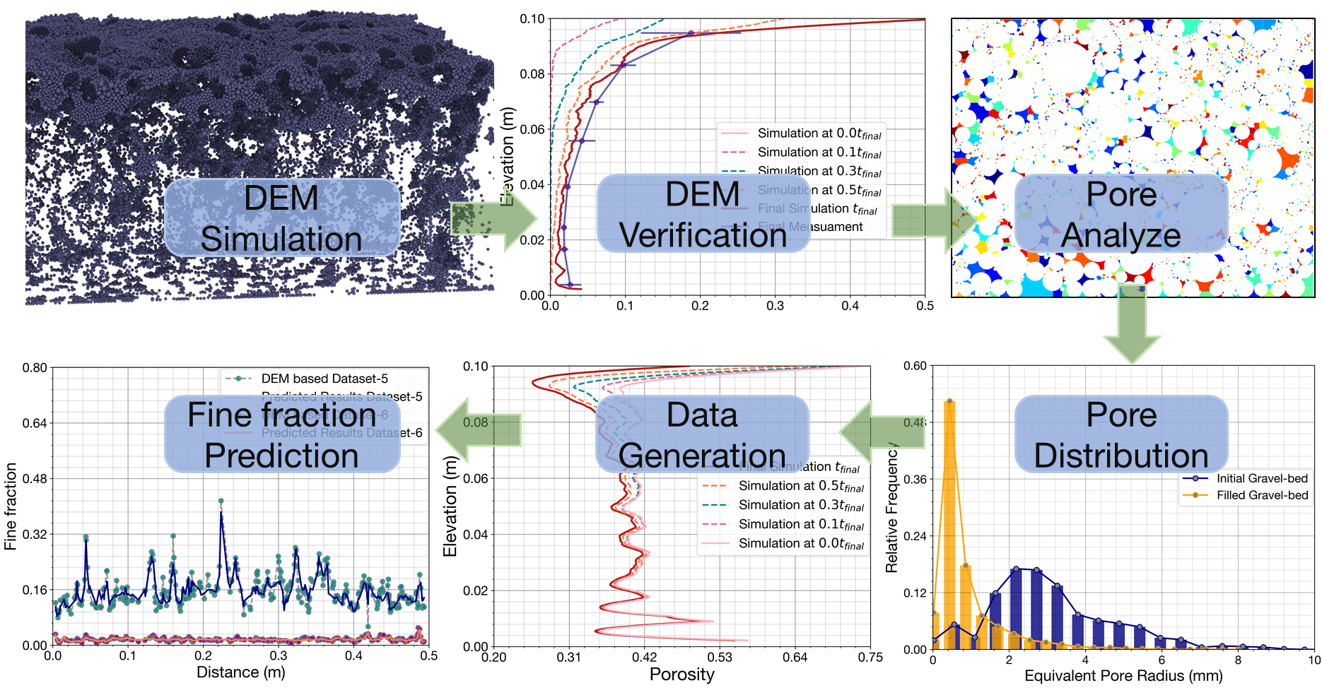
To understand grain sorting mechanisms of infiltration of fine sediment into immobile gravel-beds, we need to better analyze the relationship between the fine sediment distribution and factors including porosity, pore distribution, and size ratio. In this paper, we applied the discrete element method (DEM) to simulate the infiltration of fine sediment into gravel-bed flumes. Sediment particle properties and interaction laws were also incorporated into the DEM to simulate the collective behavior of the dissipative many-particle system so that the gravel-bed packing, grain size distribution, and porosity variation could be defined. Three cases of simulation were conducted in this paper: the first simulation (case 1), with uniform fine sediment and gravel, was used to investigate the dependence of the exchange rate on size ratio and the fine sediment fraction contained in the bed. The second and third simulations (case 2 and case 3) were conducted for multiple fine sediment sizes in proportion to the gravel-bed in order to verify the DEM model. The calculated DEM results were compared with the preceding experiment results conducted by Gibson et al. [18]. Algorithms calculating porosity, grain size distribution, and the fine sediment exchange rate between layers were used, along with the watershed segmentation method analyzing pore distribution in order to process DEM results. Finally, on the basis of the DEM results of cases 2 and 3, 12 generated datasets were used to train a feedforward neural network (FNN) to obtain the relationship between fine sediment fraction and the controlling factors. We compared the results of the FNN, DEM, and the experiment cited to verify the framework of DEM and FNN in simulating exchange rate and predicting fine sediment fraction in gravel-bed rivers.

2. Fine Sediment Distribution Controlling Factors

In this study, we considered a two-layer bed model, and thus sediment sorting occurred only in the active layer (1) and the upmost sublayer (2) (Figure 1). The bed sediment moved in the form of infiltration. Total fine sediment exchanging in the bed was divided into three parts: fine sediment that contributes to bed evolution, fine sediment trapped in the surface, and subsurface.

The Grain Size Ratio, Porosity, and Bed Saturation Condition

Following the theoretical investigations, fine sediment distribution depends on porosity and the ratio of fine sediment to coarse gravel, as well as the fine fraction contained in the bed. These studies were based on the mass conservation for fine fraction transported through gravel matrix. According to the theory of Cui et al. [3], developed from Lauck [12], the amount of the transported fine sediment trapped in immobile gravel is dependent on the riverbed characteristics, which include porosity, grain size ratio, and the fine fraction contained in the bed. Thus, the trapping coefficient was introduced, which depends on the ratio of fraction of fine sediment and the maximum amount of fine sediment that can be contained in gravel (saturation state). On the basis of the theory of Cui et al. [3], the following functions were determined for trapping coefficients of a two-layer model $({\zeta }_a and {\zeta }_s)$.

Surface layer:

$${\zeta }_a ={\zeta }_{a,0} exp\left({\varphi }_a\frac{{\beta }_a/{\beta }_{a,sat}}{1-{\beta }_a/{\beta }_{a,sat}}\right)$$

(1)

Subsurface layer:

$${\zeta }_s ={\zeta }_{s,0} exp\left({\varphi }_s\frac{{\beta }_s/{\beta }_{s,sat}}{1-{\beta }_s/{\beta }_{s,sat}}\right)$$

(2)

where ${\beta }_a and {\beta }_s$ are fine fractions in surface and subsurface layers, ${\beta }_{a,sat} and {\beta }_{s,sat}$ are the saturated fine sediment infiltration in surface and subsurface layers, ${\zeta }_{a0} and {\zeta }_{s0}$ are the trapping coefficients of the surface and subsurface layers corresponding to ${\beta }_a and {\beta }_s=0$, and ${\varphi }_a and {\varphi }_s$ are dimensionless coefficients that define the shape of trapping coefficients [3].

The saturation of fine sediment in layers depends on the porosity of the gravel and the sediment, as well as on the size ratio of fine sediment to gravel. On the basis of the function developed by Wooster et al. [19], the saturated fine sediment infiltration was determined as follows:

$${\beta }_{a,sat}=\frac{\left(1-p_f\right)p_g}{1-p_f{p}_g}{f}_n\left(D/d\right)$$

(3)

$${\beta }_{s,sat}=\frac{\left(1-p_f\right)p_g}{1-p_f{p}_g}{f}_n\left(D/d\right)$$

(4)

where $p_f$ is the porosity of fine sediment, $p_g$ is the porosity of gravel, D denotes the characteristic particle size of gravel, and d denotes the characteristic particle size of fine sediment.

These equations contain some empirical coefficients, namely, the size ratio functions (f_n); the trapping functions’ ($\zeta$) saturation state; and porosity, which can only be estimated on the basis of the observed data. The following framework, combining the FNN and DEM models, was used to obtain the functional relationship between the fine sediment distribution and the affected factors in surface and subsurface layers (Figure 2).

3. Discrete Element Method

DEM was initially proposed by Cundall and Strack [20] to model the mechanical behavior of granular flows and to simulate the forces acting on each particle and its motion. Typically, a particle can be classified into two types of motion in DEM: translation and rotation. Momentum and energy of particles are exchanged during collisions with their neighbors or a boundary wall (contact forces), through particle–fluid interactions, as well as through gravity. Applying Newton’s second law of motion, we can determine the trajectory of each i-particle (including its acceleration, velocity, and position) from the following equations:

$$m_i\frac{d{\overrightarrow{u}}_i}{dt}=m_i\overrightarrow{g}+{\displaystyle \sum }_k{\overrightarrow{f}}_{i,k}+{\overrightarrow{f}}_{i,f}$$

(5)

$$I\frac{d{\overrightarrow{\omega }}_i}{dt}=\frac{d_i}{2}{\displaystyle \sum }_k\left({\overrightarrow{n}}_{i,k}\times {\overrightarrow{f}}_{i,k}\right)$$

(6)

where m_i = the mass of a particle i, u_i = the velocity of a particle, g = gravity acceleration, f_i,k = interaction force between particle i and particle k (contact force), f_i,f = the interaction force between the particle i and the fluid, I = Momentum inertia, ω_i = angular velocity, d_i = diameter of the grain i, n_i,k = directional contact = vector connecting the center of grains i and k.

We used a contact force model based on the principle of spring–dashpot, as well as suggestions of Hertz–Mindlin [21]. The contact force was obtained from a force analysis method; the stiffness and damping factors were analyzed in two directions: orthogonal and tangent of the contact surface between the two grains:

$$f_{i,k}^{\left(n\right)}=k_i^{\left(n\right)}{\delta }_{i,k}^{\left(n\right)}+{\alpha }_i^{\left(n\right)}\Delta u_i^{\left(n\right)}$$

(7)

$$f_{i,k}^{\left(\tau \right)}=k_i^{\left(\tau \right)}{\delta }_{i,k}^{\left(\tau \right)}+{\alpha }_i^{\left(\tau \right)}\Delta u_i^{\left(\tau \right)}$$

(8)

where (n) and (τ) are known as two components of contact force in a normal direction and tangential direction, k_i = stiffness of grain i, δ_i,k = the characteristic of the contact and displacement (also called the length of the springs in the two directions above), α_i = damping coefficient, and Δu_i = relative velocity of grain at the moment of collision. Additionally, following Coulomb, the value of tangential friction is determined by the product of the coefficient of friction μ and the orthogonal force component. In the nonlinear contact force Hertz–Mindlin model, the tangential force component will increase until the ratio (f^(τ)/f⁽ⁿ⁾) reaches a value of μ, and it keeps the maximum value until the particles are no longer in contact with each other. A detail of the force models, as well as the method for determining the relevant coefficients, can be found in Johnson [21].

All forces were caclulated on the sediment particles as well as the velocity and the position of the particle at a previous time step; then, we could determine the velocity and position of grain at the present step on the basis of solving Equations (8) and (9). The grain size distribution, as well as the porosity of the bed for whole the domain, could then be defined afterward. As a result, we could then quantify the exchange rate of the fine fraction between different bed layers.

This study used the Open Source Software LIGGGHTS [21] (LAMMPS improved for general granular and granular heat transfer simulations) to perform DEM simulations, and implemented a new Hertz–Mindlin granular contact model [21,22,23], where grains were modeled as compressible spheres with a diameter d that interacts when in contact via the Hertz–Mindlin model [21,23]. Algorithms were developed to calculate grain size distribution and porosity from the calculated results of location and diameter of grains. The calculations in this study were conducted on a modern PC with Processor Intel Core.

4. Algorithm to Analyze the DEM Results

4.1. The Calculation of Exchange Rate and Time Normalization

Applying LIGGGHTS software, the locations and number of the fine sediments are updated in every time step and dumped in result files. From this result, simple equations are developed to calculate the exchange rate of fine sediment in the gravel-bed (so-called exchange rate) that describes the ratio of the number of the fine sediments trapped to the total number of sediment fed. Hence, for the sample jth, the three exchange rates that were defined for the two-layer gravel-bed model included the exchange of surface layer $E_{j,sur}^t$, the exchange of subsurface layer $E_{j,sub}^t$, and total exchange rate $E_{j,tot}^t$ by the following equations:

$$E_{j,sur}^t=\frac{N_{j,sur}^t-N_{j,sur}^{t-1}}{n_{j,fed}^t}$$

(9)

$$E_{j,sub}^t=\frac{N_{j,sub}^t-N{o}_{j,sub}^{t-1}}{n_{j,fed}^t}$$

(10)

$$E_{j,tot}^t=\frac{N{o}_{j,tot}^t-N{o}_{j,tot}^{t-1}}{n_{j,fed}^t}$$

(11)

where $N_{j,sur}^t$ and $N_{j,sur}^{t-1}$ are the number of grains trapped in the surface layer at time t and t−1, $N_{j,sub}^t$ and $N{o}_{j,sub}^{t-1}$ are the number of grains trapped in the surface layer at time t and t−1, $N{o}_{j,tot}^t$ and $N{o}_{j,tot}^{t-1}$ are the number of grains trapped in two layers at time t and t−1, and $n_{j,fed}^t$ is the total number of grain fed from time t−1 to time t.

In the conducted samples for investigating exchange rate, the simulation time is significantly different; for example, the large size ratio of fine and coarse grain (d/D = 0.45) has a simulation time of 15 min, however, with the small size ratio (d/D = 0.1), the simulation time is up to 15 h. In order to facilitate comparison, time simulation is normalized by defining the time for start exchange as 0 and the ended time simulation as 1. The normalized time for sample jth at time step k is calculated by

$$t_j^k=\frac{T_j^k-T_j^B}{T_j^E-T_j^B}$$

(12)

where $T_j^B$ is the time step at beginning of the infiltration process, $T_j^E$ is the time step at end of the infiltration process of the sample jth, and $T_j^k$ is the time step k of the infiltration process of the sample jth.

4.2. Algorithms for Calculating Size Distribution and Porosity of A Cross Section from DEM Results

Applying the algorithm developed by Bui et al. [24] for the LIGGGHTS results of 3D locations and diameter of grains, the porosity and grain size distribution can be calculated as follows.

We used the K different planes with elevations z_k (k = 0, …, K), which intersect the spherical grain matrix. The diameter of generated circle i (i = 1, …, n_k) is dependent on the spherical diameter and the relative position between the k-plane and grain i.

The diameter of each circle created by the intersection between plane k and grain ith is calculated as

$$D_{i,k}=\sqrt{D_i^2-4{\left(z_k-z_i\right)}^2} if z_i-\frac{D_i}{2} \le z_k<z_i+\frac{D_i}{2}$$

(13)

Total solid area (A_s,k) of all n_k grains in plane k is determined as

$$A_{s,k}={\displaystyle \sum }_{i=1}^{n_k}{A}_{i,k}={\displaystyle \sum }_{i=1}^{n_k}\frac{\pi D_{i,k}^2}{4}$$

(14)

The total area A_t is calculated on the basis of the shape generated by the plane k cut across the grain channel, whereby porosity of cross section k is calculated by the following equation

$$p_k=1-\frac{A_{s,k}}{A_t}$$

(15)

To calculate the grain size distribution, the grains in cross-section k are divided into m_k size fractions with characteristic grain size D_j (j = 1, …, m_k) and D_j < D_j+1, and then the area of each fraction is calculated by

$${\mathrm{A}}_{\mathrm{j}}^{\left(\mathrm{k}\right)}={\displaystyle \sum }_{\mathrm{i}=1}^{{\mathrm{n}}_{\mathrm{j},\mathrm{k}}}\frac{{\mathsf{\pi }\mathrm{D}}_{\mathrm{i},\mathrm{k}}^2}{4}{\mathrm{if}\mathrm{D}}_{\mathrm{j}-1}\le {\mathrm{D}}_{\mathrm{i},\mathrm{k}}<{\mathrm{D}}_{\mathrm{j}}$$

(16)

with

$${\displaystyle \sum }_{j=1}^{m_k}{n}_{j,k}=n_k$$

(17)

The fraction of class j in cross-section k is calculated by the following equation:

$${\beta }_j^{\left(k\right)}=\frac{A_j^{\left(k\right)}}{{{\displaystyle \sum }}_{i=1}^{m_k}{A}_i^{\left(k\right)}}$$

(18)

4.3. Watershed Segmentation to Analyze the Distribution of the Pores

Pore distribution of gravel-bed river plays a vital role for analyzing the fine sediment infiltration. To determine the pore distribution, watershed segmentation to analyze the cross section images [25] was used in this study.

The watershed segmentation method is a useful tool that is capable of detecting and distinguishing pores that touch in images. A traditional way to produce edge images is by applying a gradient and then a threshold to the outputted images to generate a binary edge image. Malpica et al. [26] claim the watershed algorithm is a fast and efficient technique to segment and separate combined clusters of pores. The watershed algorithm becomes most applicable for processing grayscale; its use in segmenting binary images by transforming binary images to grayscale using distance converter is also valid (Figure 3). First, distance transform on our binary image must be applied. The pixel brightness, as described in the distance converter, is solved by determining the length between that pixel and the nearest point of the pore’s boundary (Figure 3b). Numerous formulas exist to determine this length including Euclidean, city block, and chessboard. Rabbani et al. [27] discovered that the city block distance transforms used before watershed results in more effective segmentation of the porous rock images into two and three dimensions. Secondly, one must convert the distance map into a topological surface where brighter pixels indicate deeper parts of that surface (Figure 3c). Therefore, a basin is formed for each of the pores in the image. Accumulation of water begins in the lowest part of the basin as per the depth contours (Figure 3d). The water elevation increases in the basins until two previously isolated water lakes converge with each other. When water lakes of two different basins encounter each other, the pixel location is denoted as the watershed ridge line. At the completion of the flooding process, all watershed ridge line pixels are determined. At this point, the watershed ridge line splits the two touching pores (Figure 3e). As mentioned above, brighter points in the distance image signify points farther from the boundary of a pore. In this study, the city block distance equation was used to create the distance image. For two pixels with x and y coordination, the city block equation can be described as follows: City block distance = |x₁ - x₂| + |y₁ - y₂|.

4.4. Transferred Coefficients

In this study, the pore size of gravel-bed was used as a factor influencing the fine sediment infiltration process. However, it differs from previous researchers [28,29,30] who used the pore size definition as the largest circle diameter that fits into the voids. Applying the watershed segmentation method, the pore size is defined as the diameter of the circle that has the same area with the void space (so-called equivalent area). For convenient comparison of these results to the previous studies, the transferred coefficient can be used to convert between the two definitions of pore size mentioned above. To evaluate the range of the transferred coefficient (R), we considered the range of “close packing” (cubical packing) and of “loose packing” (tetrahedral packing) (Figure 4).

Areas of void space of cubical $A_{void}^C$ and tetrahedral packing $A_{void}^T$ are calculated by the following equations:

$$A_{void}^C=\frac{D^2\sqrt{3}}{4}-\frac{\pi D^2}{8}=\frac{2\sqrt{3}-\pi }{8}{D}^2$$

(19)

$$A_{void}^T=D^2-\frac{\pi D^2}{4}=\frac{4-\pi }{4}{D}^2$$

(20)

The diameters are defined by the equivalent pore area of cubical $d_e^C$ and tetrahedral packing $d_e^T$:

$$d_e^C=\sqrt{\frac{A_{void}^C}{\raisebox{1ex}{$\pi $}\!\left/ \!\raisebox{-1ex}{$4$}\right.}}=\sqrt{\frac{2\sqrt{3}-\pi }{2\pi }}D=0.227D$$

(21)

$$d_e^T=\sqrt{\frac{A_{void}^T}{\raisebox{1ex}{$\pi $}\!\left/ \!\raisebox{-1ex}{$4$}\right.}}=\sqrt{\frac{4-\pi }{\pi }}D=0.523D$$

(22)

The largest diameters are fitted in a pore of cubical $d_l^C$ and tetrahedral packing $d_l^T$:

$$d_l^C=2\left(\frac{2}{3}D\frac{\sqrt{3}}{2}-\frac{D}{2}\right)=\frac{2\sqrt{3}-3}{3}D=0.155D$$

(23)

$$d_l^T=\left(\sqrt{2}-1\right)D=0.414D$$

(24)

Transferred coefficients for cubical packing $R^C$ and tetrahedral packing $R^T$ are calculated by the following equations:

$$R^C=\frac{d_e^C}{d_l^C}=\frac{0.227D}{0.155D}=1.46$$

(25)

$$R^T=\frac{d_e^T}{d_l^T}=\frac{0.523D}{0.414D}=1.26$$

(26)

Transferred coefficients range from 1.26 to 1.46 for loose packing and close packing, respectively. However, the transferred coefficient is also dependent on the shape and the deformation that were not considered in this calculation.

5. Feedforward Neural Network

In recent decades, artificial neural network (ANN), a computational intelligence technique, has emerged as a powerful tool for handling complex geoscience morphology problems [24,31]. In this study, ANN was applied to predict the characteristics of gravel-bed, including grain fractions of gravel-bed in surface and subsurface layers using DEM-based data.

ANN is a general term that encompasses many different network architectures. FNN is an artificial neural network where connections between nodes do not form a cycle. FNN is the first and simplest type of artificial neural network developed. Information in an FNN travels in only one direction—forward, from input nodes, through hidden nodes, and then to the output nodes. Further, the most widely used FNN is a multilayer perceptron (MLP). An MLP model contains several artificial neurons otherwise known as processing elements or nodes. A neuron is a mathematical expression that filters signals traveling through the net. A single neuron receives its weighted inputs from the connected neurons of the previous layer, which are normally aggregated along with a bias term. The bias term is purposed to adjust the input to an appropriate range to increase the convergence properties of the FNN model. The associated summation is conveyed through a transfer function (active function) to achieve the neuron output. Weighted connections modify the output as it is moved to neuron input in the next layer, where the procedure is repeated. The weight vectors that connect the different network nodes are discovered through the so-called error back-propagation method. During training neural networks, these parameter values are varied in order for the FNN output to align with the measured output of a known dataset [32,33]. Changing the connection weights in the network according to an error minimization criterion achieves a trained response. Overfitting is avoided if a validation process is implemented during the training neural networks. When the network has been sufficiently trained to express the best reaction to input data, the network configuration is established and a test process is conducted to evaluate the performance of the FNN as a predictive model [31].

6. Results and Discussion

6.1. Study Cases

Case 1: The simulations consist of nine square boxes for investigating the exchange rate of fine sediment with different size ratios—coarse grains with uniform size D = 1.0 cm were filled in all nine boxes, and fine grains with uniform sizes d = 0.45, 0.414, 0.40, 0.35, 0.30, 0.35, 0.30, 0.25, 0.20, 0.15, 0.10 cm were filled in boxes from 1 to 9.

Case 2 and 3 were conducted in a rectangular flume with a length of 0.5 m, a height of 0.2 m, and a sediment layer thickness of 0.1 m for preparing fine fraction data.

Case 2 (bridging): Fine sediment with a mean diameter of d_m = 0.349 mm and a standard deviation of σ_(d) = 1.98; gravel-bed with a mean diameter D_m = 7.427 mm and a standard deviation of σ_(D) = 1.251.

Case 3 (percolation): Fine sediment with d_m = 0.235 mm and σ_(d) = 1.983; gravel-bed with D_m = 10.141 mm and σ_(D) = 1.462.

Case 2 and case 3 are respectively similar to experiments no. 2 and no. 3 conducted by [18] with a very slow water flowrate; hence, the effects of water flow on infiltration and packing processes could be neglected in the numerical model. The grain and water densities as well as four model parameters, whose values were determined on the basis of [34,35], can be found in

Table 1. Parameters for numerical simulation.

Density of Sphere (kg/m3)	Density of Water (kg/m3)	Young’s Modulus (Pa)	Poisson Ratio	Friction Between Grains	Coefficient of Restitution
2350	1000	5.0 × 106	0.45	0.35	0.40

.

6.2. The Exchange Rate of Fine Sediment: Case 1

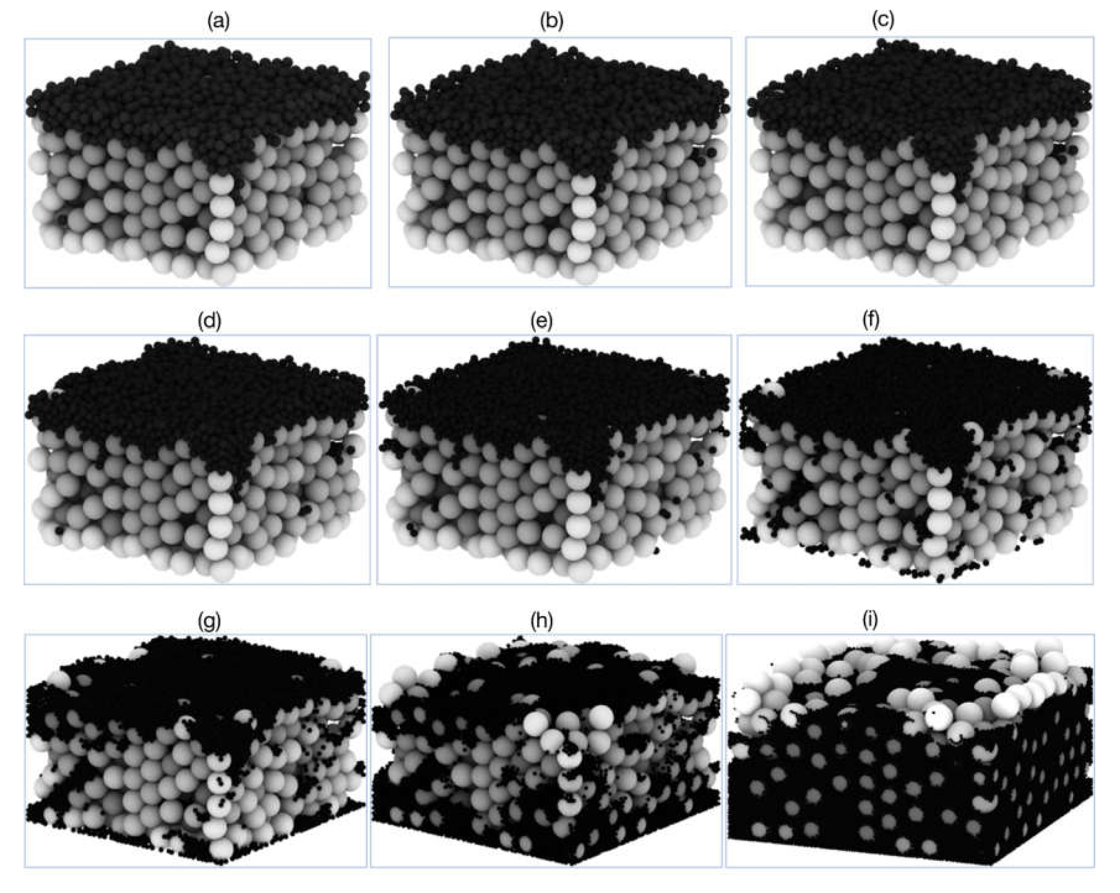
The simulation results for the fine grain size distribution of nine size ratios are shown in Figure 5. The DEM simulation was conducted in a square box with dimensions of 0.2 × 0.2 m, with the depth of the initial gravel thickness being 0.08 m. From Figure 5a–i, size of the coarse grain (D) were constant at 0.02 m, whereas the diameter of fine grain (d) reduced from 0.009 m to 0.002 m when investigating the dependence of fine sediment distribution on the size ratio. The bed porosity was 0.454. The fine sediment was fed uniformly in space and time, and the simulation was stopped when the fine sediment in gravel reached saturation. The difference in grain size distribution for size ratios 0.45, 0.414, 0.40 (Figure 5a–c) was not significant. The fine particles accumulated on the surface and could not infill to gravel. This was consistent with what was found in Allen [30], namely, how the largest possible sphere (d) that could fit in the largest void in a packing arrangement of spheres (D) was d/D = 0.52 when the void fraction was 0.4. The reason that few particles filled in the gravel was that the ratio of fine and coarse grain was smaller and the porosity was larger (0.42) than the ones in Allen’s research [30].

When the ratios were 0.35, 0.30 (Figure 5d,e) a small amount of the fine grain infiltrated into coarse bed due to fine particle bridging at the surface layer. The size ratios 0.25, 0.20, and 0.154 partially impeded percolation. For the ratios of observed percolation and bridging, these simulations are almost directly in line with previous studies [11,30,36]. The cutoff size, which denotes the coarse limit for the grain sizes that can fill in the bed pores, was smaller in DEM model than that of cubical packing (0.414) and larger than that of tetrahedral packing of solid spheres (in the original model of Yu and Standish [37] that suggested that the assumption of tetrahedral packing would be reasonable for natural mixtures [38,39]). Size ratio (d/D) for “unimpeded statistic percolation” was smaller than 0.1 (Figure 5i), which was found as a small complement for the conclusions in research conducted by [36].

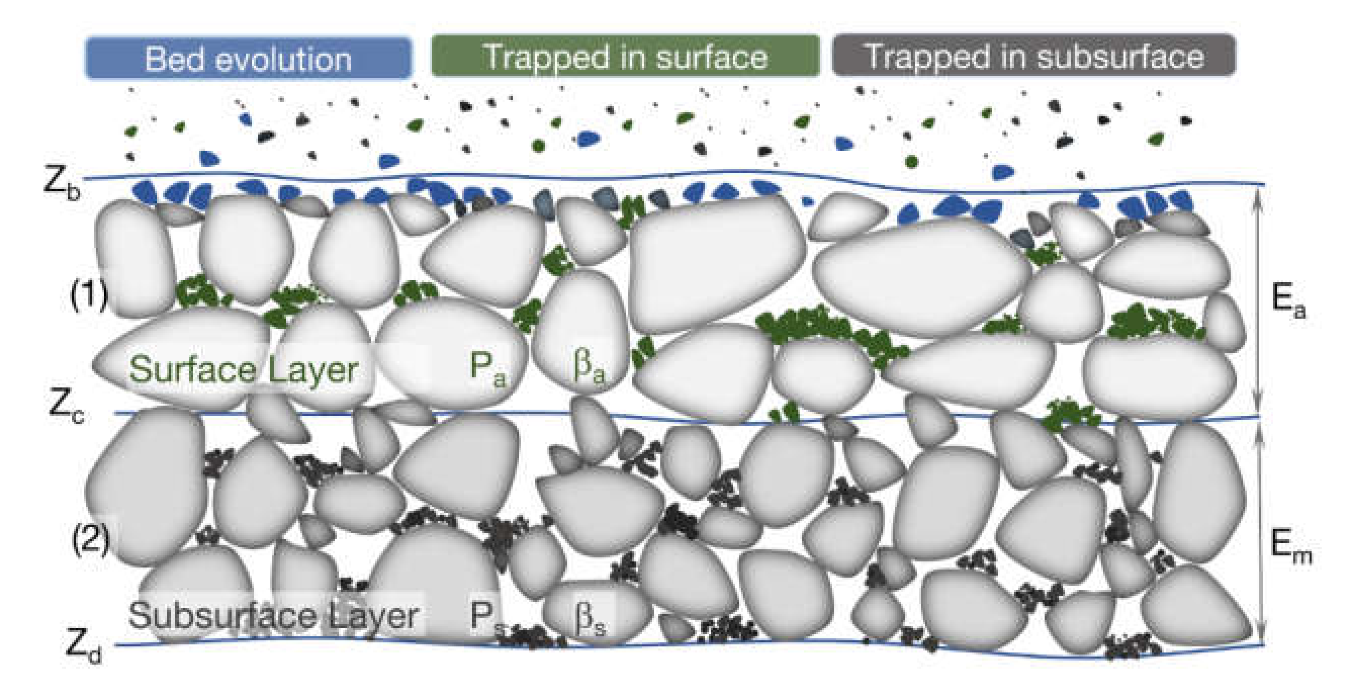
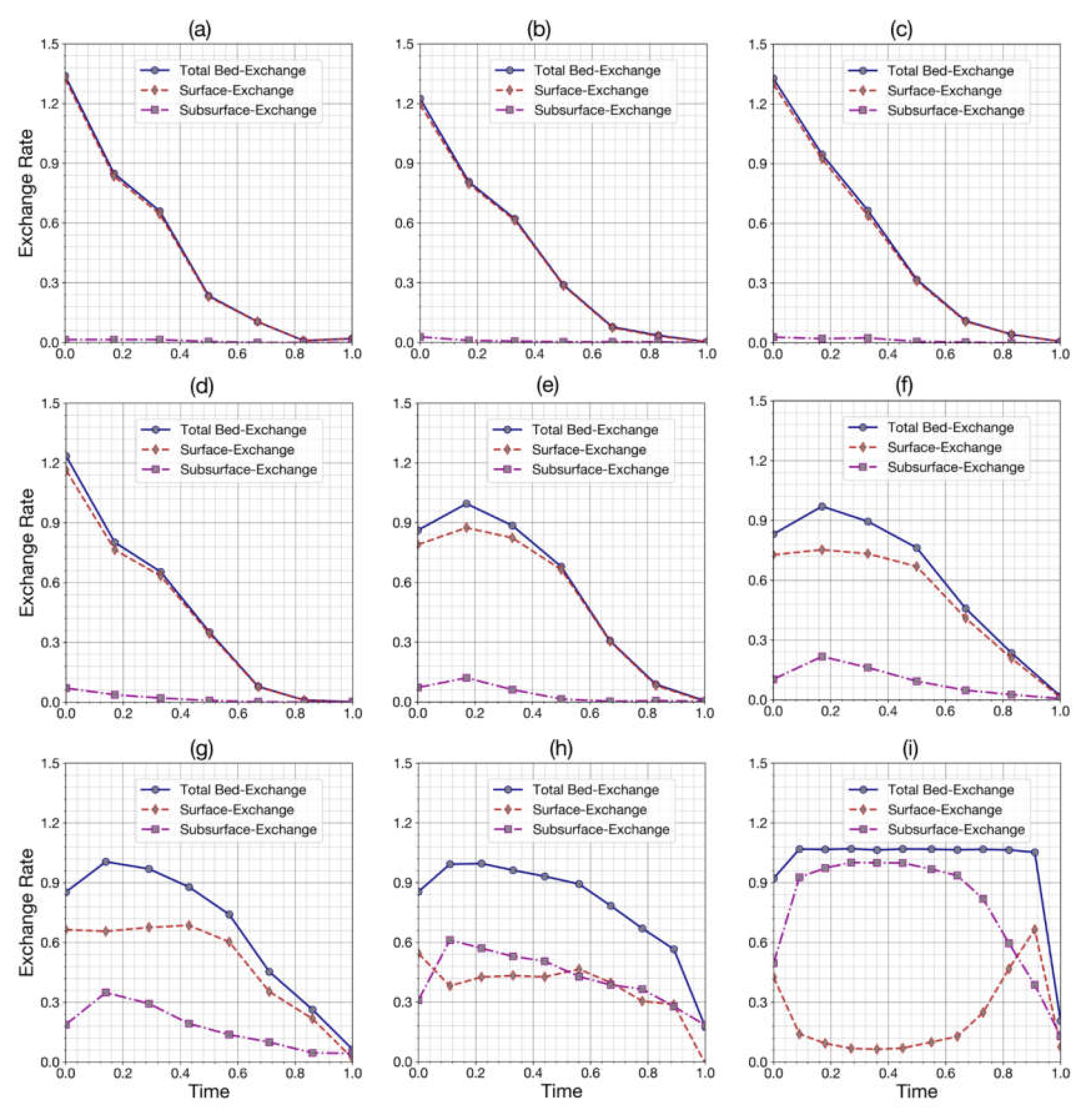
Figure 6 shows the variation of exchange fraction of fine sediment in two layers by time of nine samples with different ratios (d/D). Therefore, the bed was divided into two layers: the thickness of the surface layer was two times of the coarse diameters (D), whereas the remaining space from the bottom of the surface layer to the bottom of the box was a subsurface layer that was approximately five times the coarse diameter. At the initial time, the fine grain was fed into the pure gravel. After that, the gradual increase over time of the fine fraction contained on the void space of gravel reduced the exchange rate, as can be seen in Figure 6.

As can be seen in Figure 6a–d, with a size ratio 0.45–0.35, the maximum of the exchange rate was at the first time step (one step in visualization was equivalent to 40,000 time steps in the simulation), and the exchange of fine sediment only occurred in the surface layer (dashed line with diamond marker). For size ratios 0.30–0.10 (Figure 6e–i), the maximum exchange rate in the surface was in the second time step. The time delay at the first time step was due to the accumulation of fine grain on the top layer, when the flux of the infiltration had not yet formed. The exchange rate in the subsurface layer was not significant in the ratios (d/D) 0.45–0.35 (Figure 6a–d), as fine grains clogged the surface layer and could not infill in the lower layer. The increase of the exchange rate in the subsurface layer was rapid for ratios 0.30 to 0.10, with the maximum nearly reaching the feed rate in Figure 6i. In general, with size ratios larger than 0.45, the infiltration process only occurred in the surface layer. The effect of the size ratio on the exchange rate was strongly correlated with size ratios larger than 0.4, and was not significant when it was smaller than 0.1. With a size ratio smaller than 0.1, the surface layer had almost no effect on the infiltration process. Increasing fine sediment contained in the gravel over time significantly reduced the speed of the infiltration process and stopped altogether when the fine fraction of the gravel reached saturation.

6.3. Fine Fraction Distribution: Case 2 and Case 3

The second and third simulations were conducted for multiple sizes of fine sediment and gravel-bed. The DEM-calculated results were compared with the preceding experiment results conducted by Gibson et al. [18]. Algorithms were developed for calculating porosity and grain size distribution in the depth and along the flume to prepare data for data-driven methods. Image processing was used to analyze pore distribution, which is particularly difficult to determine [15]. Finally, 12 generated datasets, based on the DEM results of cases 2 and 3, were used to train an FNN model to obtain the relationship between fine fraction and controlling factors.

Figure 7 shows the 3D results of simulating the infiltration of fine sediment into gravel-bed using spherical particle. Figure 7a shows the gravel-bed, which generated a random distribution under various forces. These forces were gravity, which is the main cause of sediment settling (which reduces the distance between grains and therefore porosity); buoyancy, which reduces the effect of gravity; and grain friction, which resists the relative motion and may increase porosity. Figure 7b shows the sediment and the fine sediment distribution in the gravel (case 2). For the first 320,000 time steps, 569 grains were fed uniformly onto the surface. Then, 580 grains percolated per time step until the 980,000th time step. Figure 7c shows the fine sediment distribution in case 2, where fine particles clogged the top layer. Figure 7d shows another fine sediment distribution. In the bottom of the simulation domain, fine sediment could not move down due to bottom walls creating a sudden increase of fine fraction near the flume bed. The vertical walls around of the flume supported the infiltration process and high concentration of fine grain can be observed in Figure 7c,d. This significant increase of fine fraction in two sides of a flume always appears in experiments conducted with fine sediment and gravel-bed [4,19,40]. As can be seen in Figure 7c,d, the fine sediment distribution result based on DEM was relatively good and realistic.

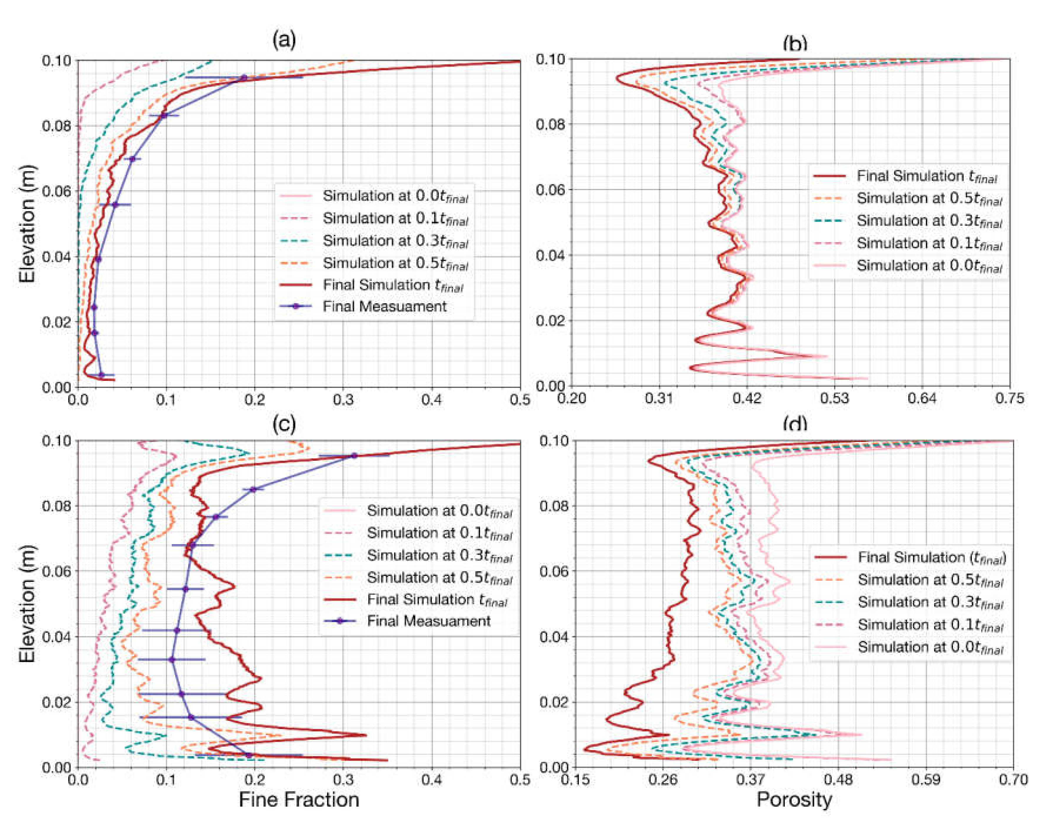
Figure 8 shows DEM simulation and experiments conducted by Gibson et al. [18] in cases 2 and 3. As can be seen in Figure 8a, with the fine fraction variation in five time steps, the speed of infiltration was reduced with time due to the increasing of the trapped fine sediment in the void space of gravel. At the top layer, the fine sediment fraction reached its highest value (0.5) because of the convex and concave shapes of the surface gravel. At the bottom layer, the fine fraction slightly increased due to the accumulation of fine sediment in the flume bed. The calculated vertical distribution of fine sediment agreed well with the observations. In Figure 8b, the porosity varied significantly at the top layer (from elevation 0.08–0.1 m) and showed small variation at the bottom layer (from elevation 0.0–0.08 m). These values correspond with the fine sediment fraction variation in Figure 8a.

Opposite results of fine sediment distribution were found in case 3 (Figure 8c), where a larger amount of fine sediment was stored at the surface layer (0.19) and in the sublayer (0.22). As a result of a large amount of fine sediment infiltration, porosity varied significantly in both the top layer and the bottom layer. In the bottom layer, porosity changed more drastically than the top layer and reached a minimum value of 0.16 (Figure 8d). As can be seen from Figure 8c, the calculated vertical distribution of the fine fractions in the bottom layer was very irregular, compared to the experimental measurements of [18]. In this case, the DEM model provided poor results in the bottom layer. The reasons for this mismatch could be as follows:

(1)

The model of bed effects, resulting in a reduced chaotic stacking particle in the above bottom layer, needed to be developed.

(2)

The spherical shape of particles used in the DEM model had effects on the capacity of the infiltrating process, allowing fine sediment to easily fill the bottom layers without clogging the top.

(3)

The experiments and measurements were conducted in a large flume with slow flowing water and without sediment transport, whereas due to high computational requirements, the DEM model considered only a small window, 0.15 m wide and 0.5 m long with quiescent water.

To evaluate the performance of the DEM model in terms of accuracy and consistency in predicting fine sediment infiltration, three statistical measures were employed: coefficient of determination (R²), root mean square error (RMSE), and mean absolute error (MAE). As can be seen from

Table 2. Verification of fine sediment distribution with Gibson’s measurement [18].

Statistical Indicators	Case 2 (Bridging)	Case 3 (Percolation)
R2	0.941472	0.866244
RMSE	0.049372	0.041221
MAE	0.035878	0.028537

, the DEM model provided an acceptable agreement between the experimental and numerical results. These validated results of the DEM model were used to design the FNN model, which is introduced in the next section.

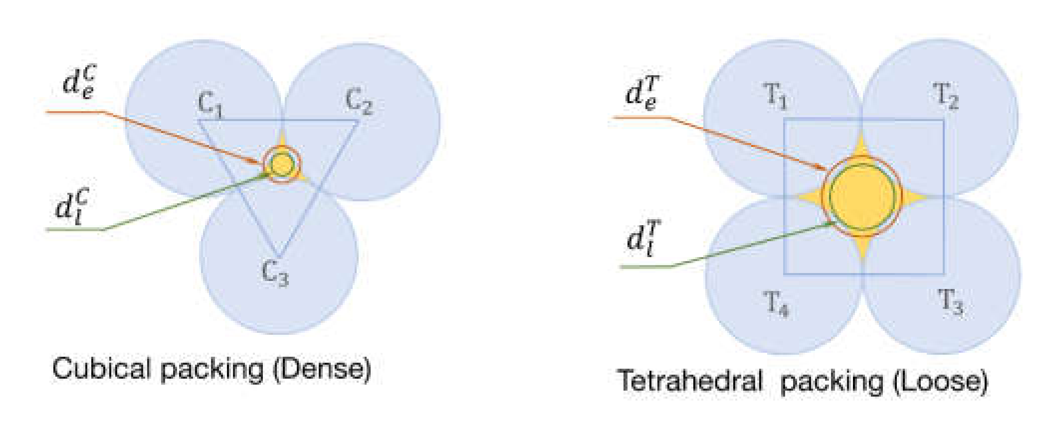
6.4. Pore Size Distribution: Case 2 and Case 3

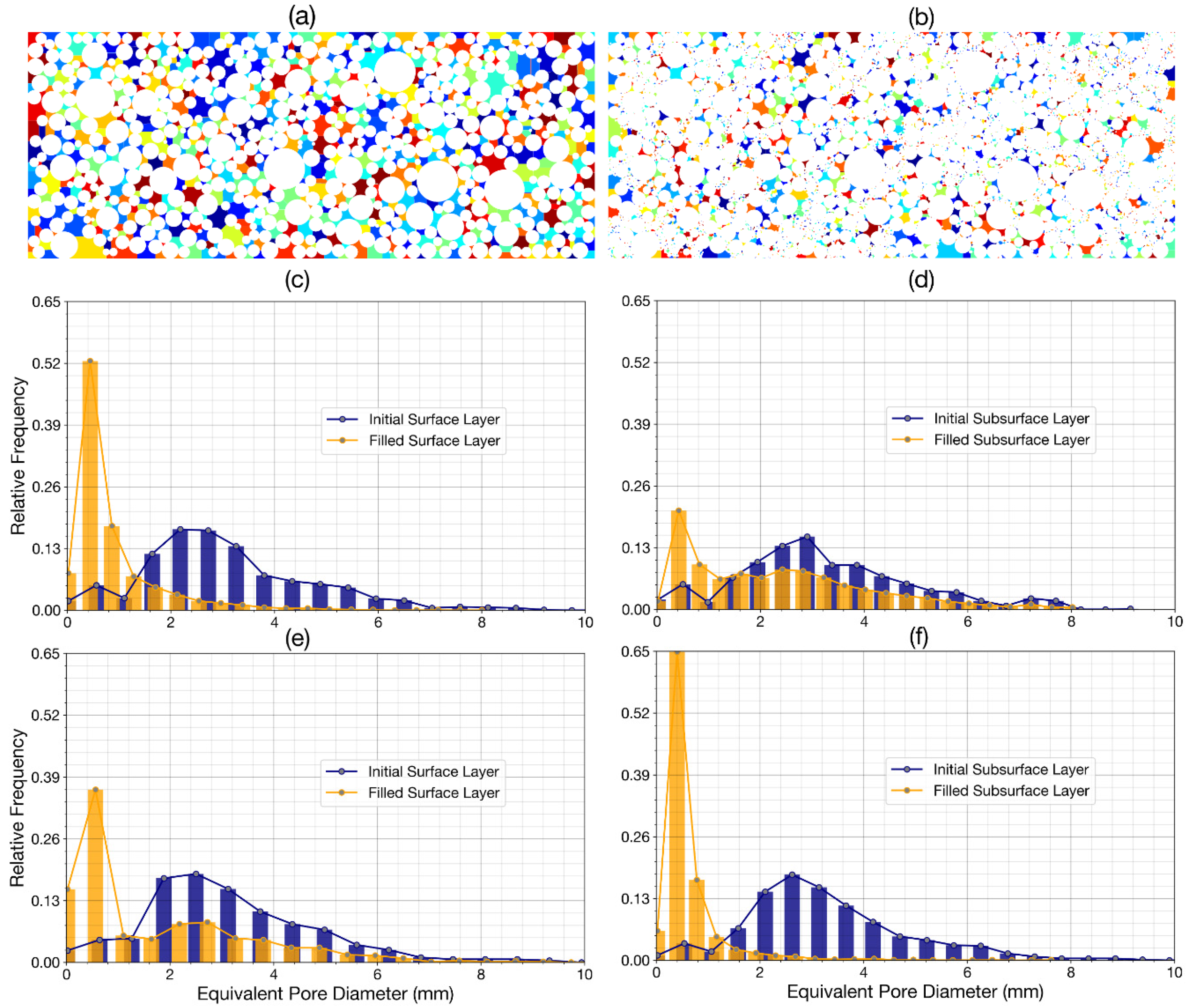
Figure 9 shows the detection and separation of pores on the basis of the watershed segmentation method. Figure 9a,b shows pore detection as the result of a middle surface cross-section before and after infiltration. After the infiltration process, the void space area decreased significantly, as can be seen in Figure 9a,b. The pore distribution near the side of the flume did not change significantly due to the effect of the wall, whereas the vertical plane of the boundary flume was easily shaped into a column to transport fine from the surface to the bottom.

We chose cross-sections at the middle surface layer and subsurface to analyze the change of pore size before and after the infiltration process of the flume in cases 2 and 3. Four cases were analyzed in Figure 9c–f. The navy color charts represent the frequency of pore distribution before the infiltration process, whereas the orange color charts represent the frequency of pore distribution after infiltration. The frequency decreased significantly for pore sizes from 1.6 to 8 mm, and increased sharply for pore sizes smaller than 1 mm. This suggests that the main contributors to the infiltration process were pore sizes larger than seven times the grain diameter (fine grain diameters used in this simulation were between 0.235 and 0.349 mm). The calculated results of the pore diameter shown in Figure 9 were based on the equivalent area pore. To compare this result of pore distribution with the previous studies, we converted from the area equivalent pore size to the largest size that fitted into the voids, which was dependent on the size ratio and packing profile (loose or dense). Using the transferred ratio calculated in Section 4.4 and the transferred ratio (from 1.26 to 1.46), we obtained the range for the minimum pore diameter contribution on the infiltration process (4.79–5.55). This result is in agreement with the previous study of [28], who also used perfectly spherical and uniform glass beads as the clogging material in spherical slots, obtaining a similar range (4–5) for minimum pore diameter. The 5.5 cutoff value for d_l:d_f was tested in experiments W-3 and W-23 conducted by Wooster et al. [19], and a median pore size to fine geometric diameter of 6.5 was used in the threshold proposed by Huston and Fox [15]. Conversely, a reinterpretation of the [41] threshold value resulted in a ratio of pore size to fine sediment size of 2.7. The difference in the simulated result and experiment was due to the friction, shape of grain, and the methodology to calculate pores. However, in general, the good agreement of the simulated results and measurements of [19,28] demonstrated that watershed segmentation is an effective method in analyzing the DEM results to obtain pore size distribution, which is useful for analyzing the infiltration process.

6.5. Data for FNN

The results obtained by the DEM for cases 2 and 3 were used to develop FNN models. Input parameters to predict the fine sediment fraction (fine fraction) along the depth (z-direction) included the location of the sample (l), the size ratio of fine to coarse grain, and porosity of the layer. A total of 500 samples of each dataset were generated from 500 different cross-sections, along with the depth (z-direction). In this part, the fine sediment fractions at half-time and final-time of the infiltration process for cases 2 and 3 were predicted. Thus, the total four datasets of the z-direction were created: the first dataset for case 2 at half-time simulation (called dataset 1), the second dataset for case 2 at final time simulation (called dataset 2), the third dataset for case 3 at half-time simulation (called dataset 3), and the fourth dataset for case 3 at final-time simulation (called dataset 4).

In the x-direction, the fine sediment fraction in surface layer and subsurface layer at half-time and final-time of the infiltration process were predicted. Thus, a total of eight datasets of the x-direction were created (each dataset contained 1500 samples). For the x-direction the generated datasets were the 5th dataset for surface layer of case 2 at half-time simulation (called dataset 5), the 6th dataset for subsurface layer of case 2 at half-time simulation (called dataset 6), the 7th dataset for surface layer of case 2 at final-time simulation (called dataset 7), the 8th dataset for subsurface layer of case 2 at final-time simulation (called dataset 8), the 9th dataset for surface layer of case 3 at half-time simulation (called dataset 9), the 10th dataset for subsurface layer of case 3 at half-time simulation (called dataset 10), the 11th dataset for surface layer of case 3 at final-time simulation (called dataset 11), and the 12th dataset for subsurface layer of case 3 at final-time simulation (called dataset 12).

Each dataset in the z-direction (500 samples) was randomly divided into two subsets of data, namely, 80% (400 data) for training and 20% (100 samples) for testing purposes. Similarly, 1500 samples in the x-direction of each dataset were randomly divided into two subsets—80% (1200 samples) for training and 20% (300 samples) for testing purposes.

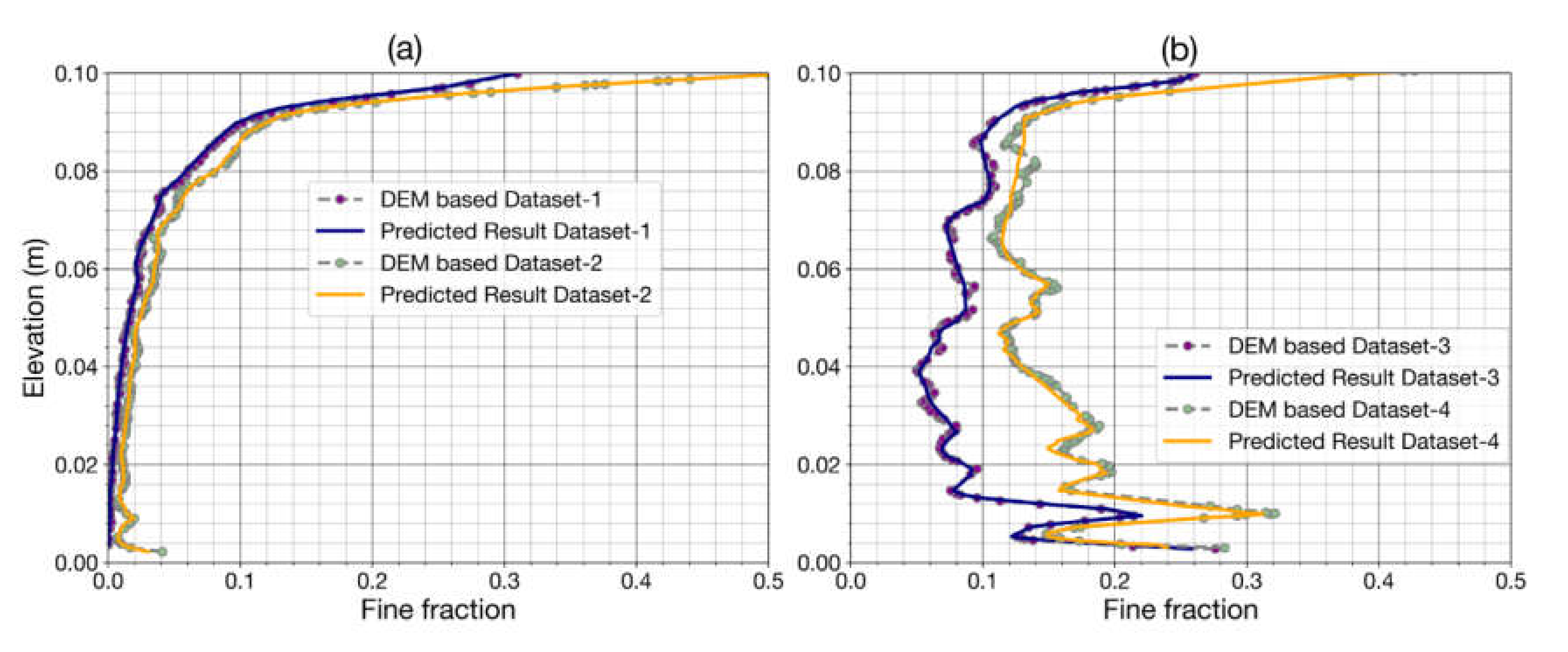
6.6. FNN for Prediction of Fine Sediment Distribution

Figure 10 shows the performance of the FNN model and the scatter of the fine sediment fraction (fine fraction) for the test dataset. As can be seen in Figure 10a, the FNN in case 2 produced a very good result in predicting the fine fraction variation with depth at half time of simulation (dataset 1) and final time simulation (dataset 2). In case 3, the performance of the FNN model was good for dataset 3, and not good for dataset 4 (Figure 10b). Overall, as can be seen in

Table 3. Statistical performances of FNN model (for testing data) along the depth (z-direction).

Dataset	1	2	3	4
R2	0.9996	0.9998	0.9970	0.9957
RMSE	0.0026	0.0021	0.0041	0.0075
MAE	0.0016	0.0016	0.0033	0.0053

, FNN models provided good results for the fine fraction prediction. This suggests that the data-driven method based on porosity and ratio was suitable for the fine fraction prediction along the depth in a gravel-bed.

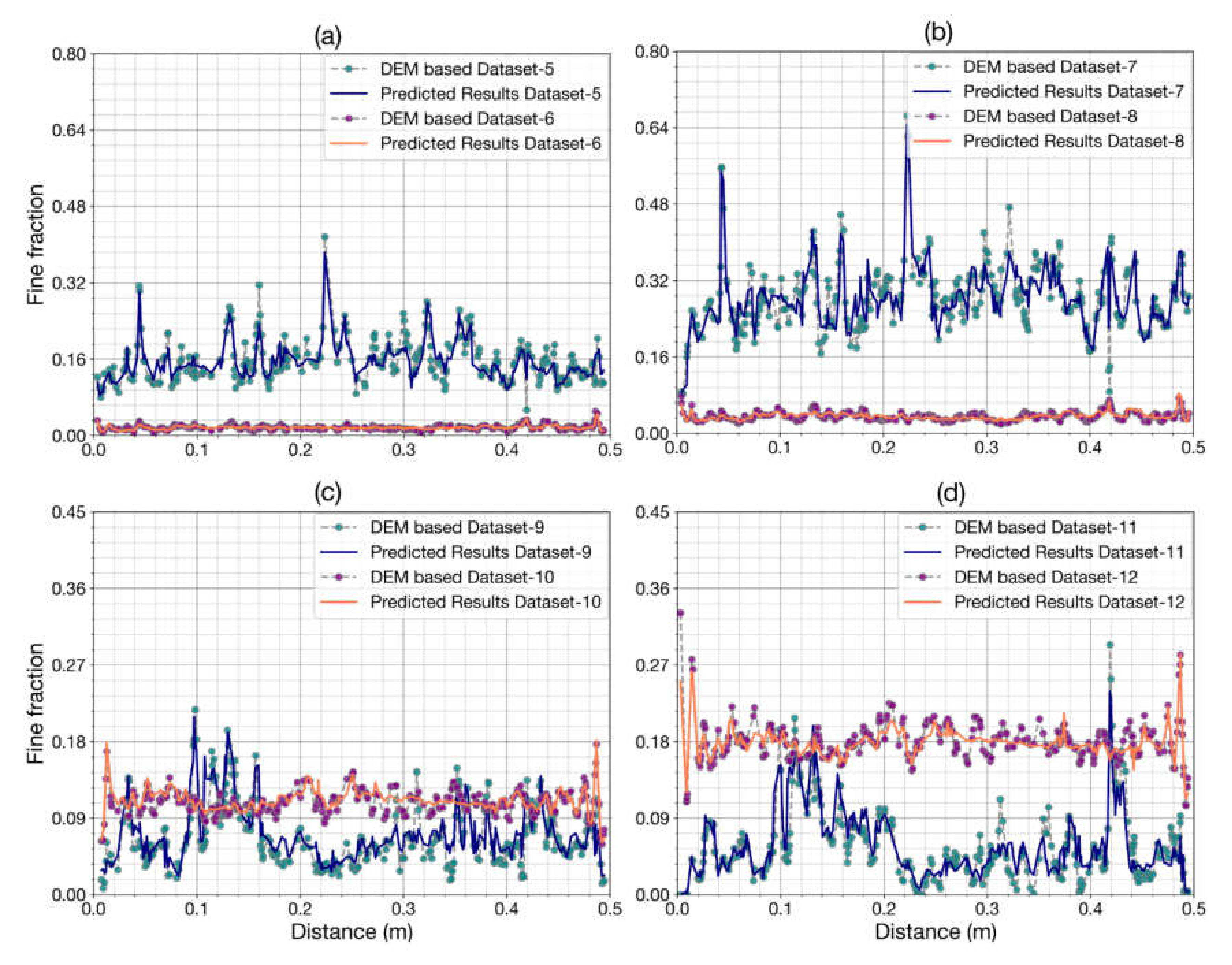
Figure 11 shows the comparison between the FNN based on the fine sediment fraction and the data obtained from DEM. Here, eight predicted fine fractions along the x-direction (datasets 5 to 12) were considered. In case 2 (Figure 11a,b), the blue dot–dash line represents the DEM-based data of the fine fraction in the surface layer, which had an average value of around 0.2 at half-time simulation and around 0.3 at end simulation. In the subsurface layer, the fine sediment fraction was small, with a minor fluctuation (0.01 at half-time and 0.04 at the end of simulation). In case 3 (Figure 11c,d), the fine fraction in the subsurface (magenta dot–dash line) was significantly higher than in the surface layer (blue dot–dash line). The average values of the fine fraction contained in the subsurface layer were around 0.1 at half-time of simulation and 0.18 at the end-time of simulation, whereas at the surface layer, the values were 0.06 and 0.07, respectively. The amplitude of fluctuation of the fine fraction in the surface was larger than in the subsurface (Figure 11). The reason for this phenomenon was the convex and concave surface layer. As a result of the movement from high elevation to low elevation, low concentration of the fine sediment was accumulated at convex zones and high concentration of the fine sediment at the concave zones. The thin surface layer also increased the amplitude of the fine fraction. The values of the fine fraction for the subsurface of percolation near the sidewall (magenta dot–dash line in Figure 11c,d) were significantly higher than inside a domain. The effect of the sidewall on the increasing of the fine fraction has also been discussed in previous experimental studies [19,41].

Figure 11a–d shows the performance of the FNN model of the fine sediment fraction prediction for the test dataset. The FNN prediction significantly underestimated the high peak (distance 0.21–0.38, dataset 5, Figure 11a; distance 0.32–0.36, dataset 7, Figure 11b) in comparison with the DEM-based data. In some ranges, FNN did not catch the rule of distribution (distance 0.27–0.39 m, dataset 10, Figure 11c; distance 0.26–0.36 m, dataset 12, Figure 11d). The fundamental reason for the tolerances was the quality of the input data. The average porosity of the input parameters of the FNN model may not have contained enough information for the fine fraction prediction. Furthermore, the DEM data may have been disturbed by the bottom and side wall effect that reduced the accuracy of the FNN model. However, in general, the performances of models were in good agreement with the DEM-based data.

Table 4. Statistical performances of FNN model (for testing data) along the flume (x-direction).

Dataset	5	6	7	8	9	10	11	12
R2	0.846054	0.768286	0.868027	0.731358	0.858198	0.865393	0.839534	0.813168
RMSE	0.024601	0.003765	0.037303	0.006473	0.022397	0.012529	0.020831	0.008961
MAE	0.018722	0.002858	0.028208	0.005376	0.016064	0.009794	0.01503	0.007007

shows relatively good results of the fine fraction prediction and in the x-direction.

Twelve datasets were used to train the network to predict fine sediment distribution, including four datasets in the z-direction and eight datasets in the x-direction. The time for each training was 3 h for FNN 10,000 iterations. The time to obtain the tested results from the predicted model was approximately 0.5 seconds. The time needed to calculate porosity was reduced from a few days in the DEM simulation to less than 1 second by employing a data-driven method for porosity prediction (

Table 5. Total time simulation and number of grains.

Simulation Parameters	Case 1							Case 2	Case 3
	d/D = 0.45	0.4	0.35	0.3	0.25	0.2	0.1
Grains	2524	3095	4053	5430	8541	15,593	15,4903	18,4931	573,822
Time (h)	0.280	0.340	0.416	0.491	0.611	0.856	10.810	14.547	198.311

). It is necessary to emphasize that a data-driven method can totally replace DEM in porosity calculation. This replacement was only applied in the same domain because only the grain size distribution varied. Nonetheless, the reduced simulation time not only saved computer resources but also made the connection between DEM and the conventional hydrodynamics model more robust. The explicit relationship between porosity and grain size distribution obtained through the trained model was used to calculate the porosity coupling with another bed porosity variation model [42] for each time step.

7. Conclusions

Estimating amount of fine sediment stored in gravel-bed is important and complex in terms of river engineering. This study succeeded in applying the combination framework of the discrete element method and artificial neural networks for simulating the infiltration process, estimating the exchange rate between the layers, and predicting the fine sediment fraction. The DEM results agreed well with the experimental results. The developed algorithms and image processing were successfully applied for extracting data from the DEM results, which were applied to design an FNN. The designed FNN showed advantages in obtaining an explicit relationship (in the form of a matrix equation) between the fine sediment distribution and the controlling factors. This equation can be applied for other inputs so that time consuming can be reduced.

Although the DEM model applied in this study still has some shortcomings (e.g., computational requirements, lack of robust parameterization procedures for model inputs, non-corresponding size of the particles compared to actual soil grains, and underestimated number of particles due to computational constraints), the effectiveness of the model in the field of graded sediment transport was shown. Because the DEM provided detailed results including position, diameter, velocity, and shear stress of particles, we extracted information about the gravel-bed packing, grain size distribution, and porosity variation, which are useful for modelling transport processes in gravel-bed. As the next step of the study, complex artificial neural networks, such as convolutional neural network, could be applied in order to segment the void spaces, fine sediment, and gravel fractions. The result images could then be used to calculate grain size distribution and pore distribution, as well as to estimate the amount of fine sediment stored in the void space of gravel from real pictures of the river bed. The application of this model could help stakeholders and managers to effectively maintain fine sediment stored in the riverbed and assess the effect of void spaces in gravel as the habitat of aquatic species for eco-hydraulic management.