Evaluation of Radar-Gauge Merging Techniques to Be Used in Operational Flood Forecasting in Urban Watersheds


Abstract
1. Introduction
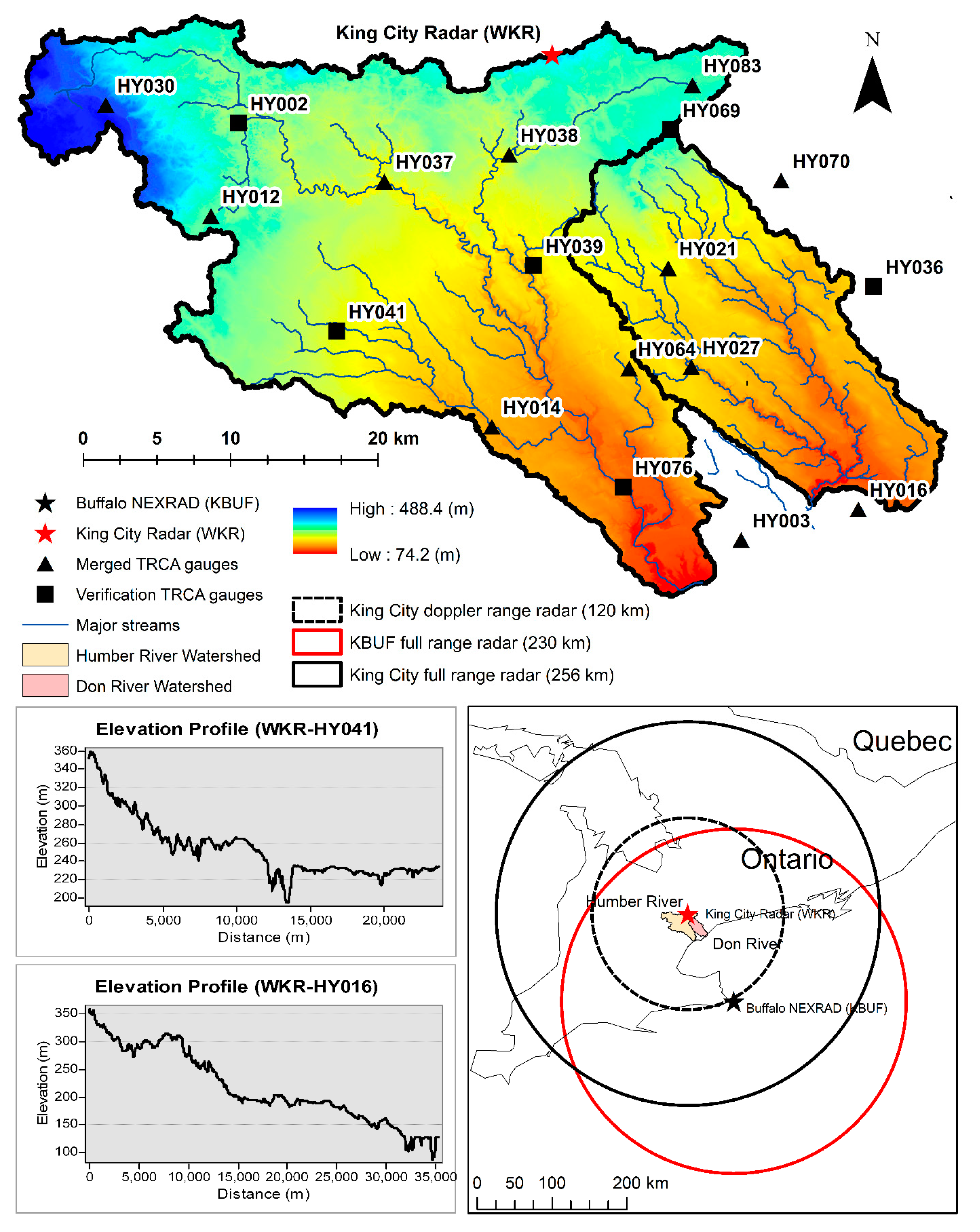
2. Study Area
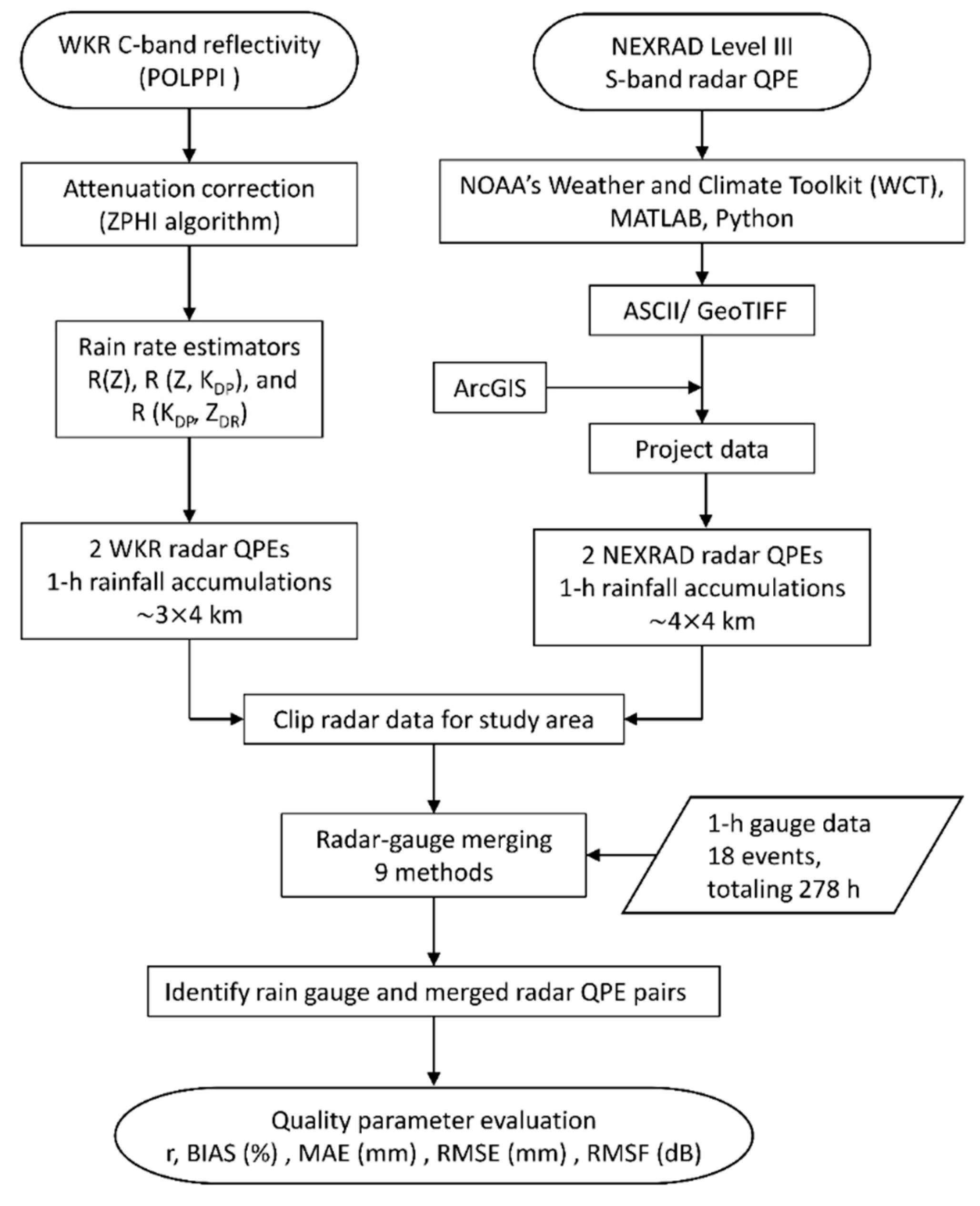
3. Materials and Methods
3.1. Data
3.1.1. Rain Gauge Data
3.1.2. King City WKR C-Band Dual-Polarized Radar QPEs
3.1.3. KBUF NEXRAD S-Band Dual-Polarized Radar QPEs
3.2. Radar-Gauge Merging Methods
3.2.1. Mean Field Bias Correction (MFB)
3.2.2. Frequency and Intensity Correction (FIC)
3.2.3. Local Intensity Scaling (LOCI)
3.2.4. CDF Matching (CDFM)
3.2.5. Range-Dependent Bias Adjustment (RDA)
3.2.6. Modified Brandes Spatial Adjustment (MBSA)
3.2.7. Kriging
Ordinary Kriging (OK)
Kriging with Radar-Based Error Correction (KRE)
3.3. Evaluation of Radar-Gauge Merging Techniques
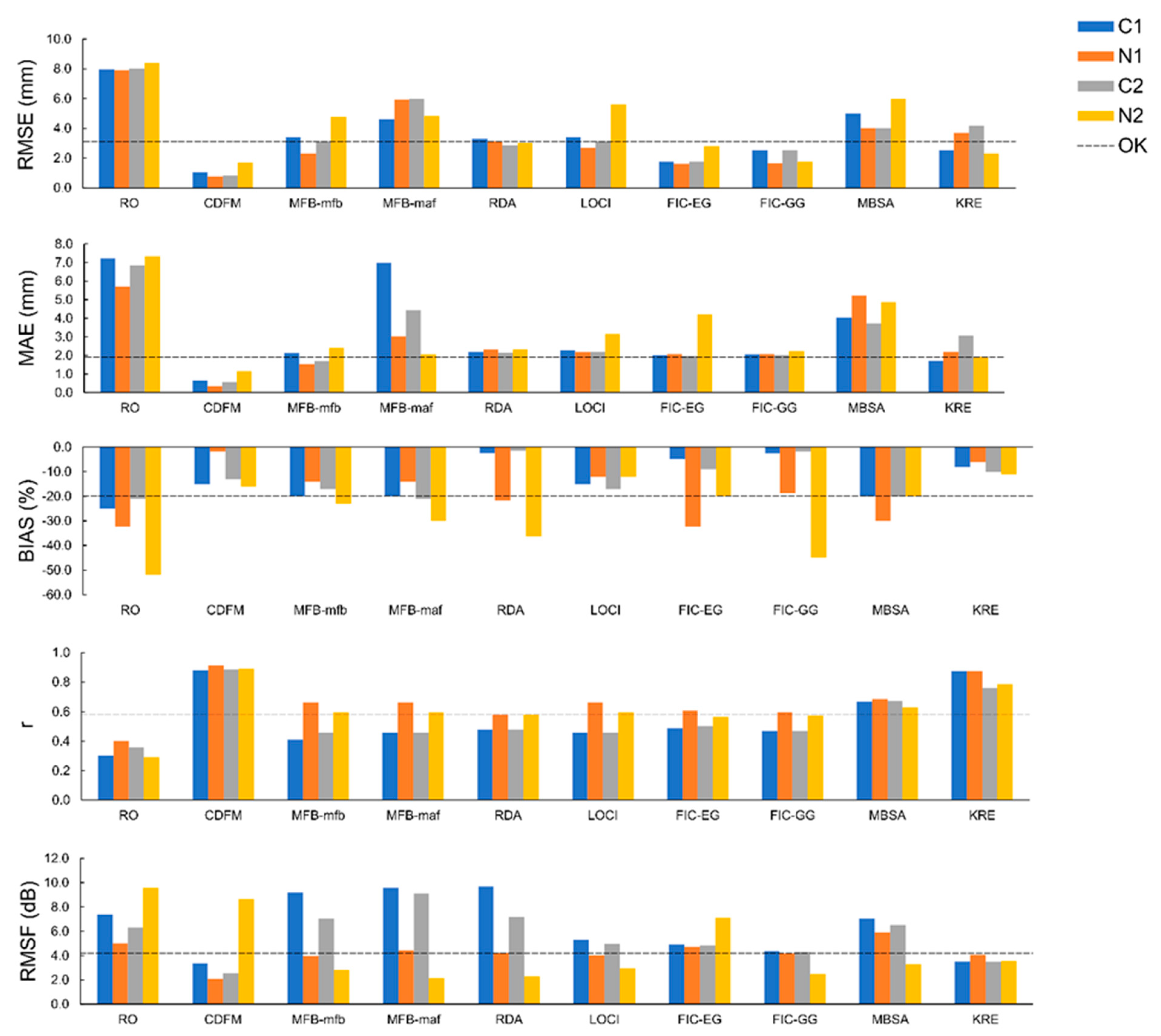
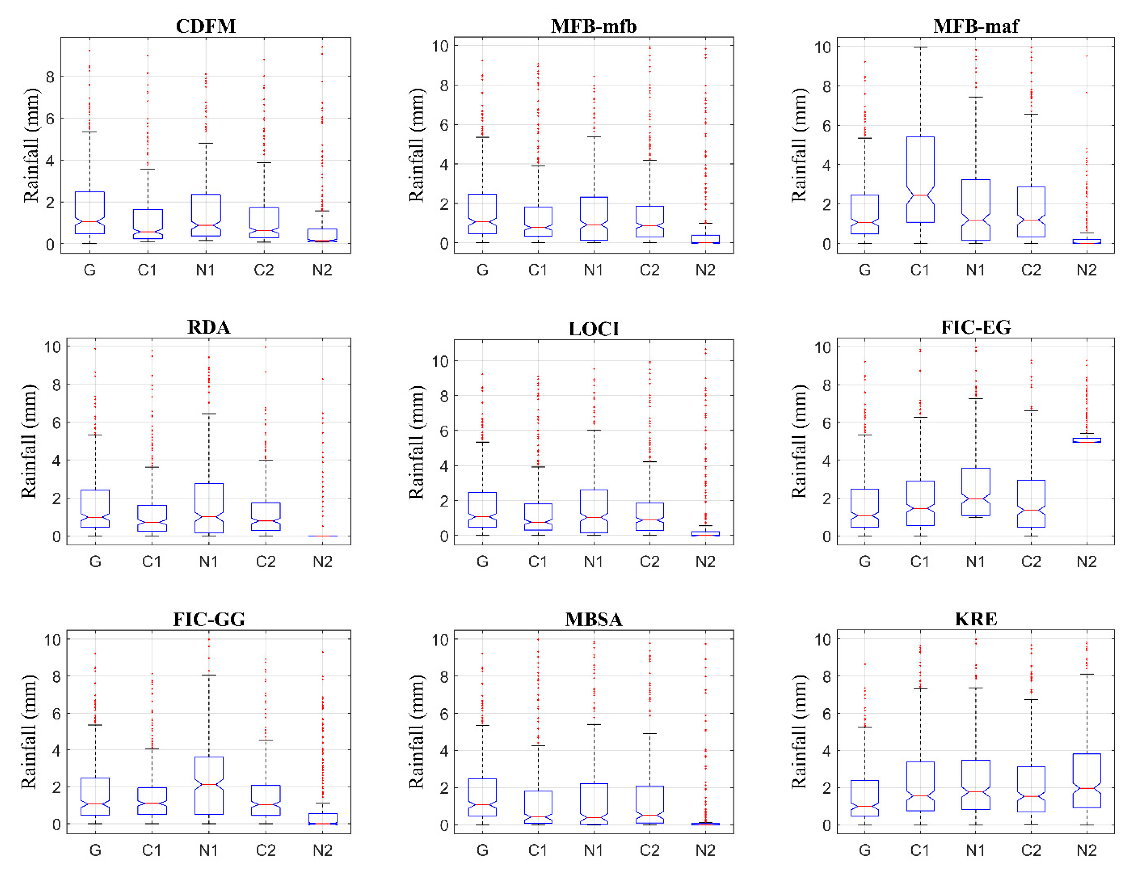
4. Results and Discussion
5. Conclusions
Author Contributions
Funding
Acknowledgments
Conflicts of Interest
References
- Balica, S.F.; Popescu, I.; Beevers, L.; Wright, N.G. Parametric and physically based modelling techniques for flood risk and vulnerability assessment: A comparison. Environ. Model. Softw. 2013, 41, 84–92. [Google Scholar] [CrossRef]
- Zahmatkesh, Z.; Kumar Jha, S.; Coulibaly, P.; Stadnyk, T. An overview of river flood forecasting procedures in Canadian watersheds. Can. Water Resour. J. Rev. Can. Resour. Hydr. 2019, 44, 213–229. [Google Scholar] [CrossRef]
- Arduino, G.; Reggiani, P.; Todini, E. Recent advances in flood forecasting and flood risk assessment. Hydrol. Earth Syst. Sci. Discuss. Eur. Geosci. Union 2005, 9, 280–284. [Google Scholar] [CrossRef]
- Awol, F.S.; Coulibaly, P.; Tsanis, I.; Unduche, F. Identification of hydrological models for enhanced ensemble reservoir inflow forecasting in a large complex prairie watershed. Water 2019, 11, 2201. [Google Scholar] [CrossRef]
- PC, S.; Nakatani, T.; Misumi, R. The role of the spatial distribution of radar rainfall on hydrological modeling for an urbanized river basin in Japan. Water 2019, 11, 1703. [Google Scholar] [CrossRef]
- Yang, L.; Tian, F.; Niyogi, D. A need to revisit hydrologic responses to urbanization by incorporating the feedback on spatial rainfall patterns. Urban Clim. 2015, 12, 128–140. [Google Scholar] [CrossRef]
- McMillan, H.; Jackson, B.; Clark, M.; Kavetski, D.; Woods, R. Rainfall uncertainty in hydrological modelling: An evaluation of multiplicative error models. J. Hydrol. 2011, 400, 83–94. [Google Scholar] [CrossRef]
- Zhu, D.; Peng, D.Z.; Cluckie, I.D. Statistical analysis of error propagation from radar rainfall to hydrological models. Hydrol. Earth Syst. Sci. 2013, 17, 1445–1453. [Google Scholar] [CrossRef]
- Beven, K. Towards an alternative blueprint for a physically based digitally simulated hydrologic response modelling system. Hydrol. Process. 2002, 16, 189–206. [Google Scholar] [CrossRef]
- Gilewski, P.; Nawalany, M. Inter-comparison of rain-gauge, radar, and satellite (IMERG GPM) precipitation estimates performance for rainfall-runoff modeling in a mountainous catchment in Poland. Water 2018, 10, 1665. [Google Scholar] [CrossRef]
- Randall, M.; James, R.; James, W.; Finney, K.; Heralall, M. PCSWMM Real Time Flood Forecasting–Toronto, Canada; CUNY: New York, NY, USA, 2014. [Google Scholar]
- Dhiram, K.; Wang, Z. Evaluation on radar reflectivity-rainfall Rate (ZR) relationships for guyana. Sciences 2016, 6, 489–499. [Google Scholar] [CrossRef]
- Thorndahl, S.; Einfalt, T.; Willems, P.; Nielsen, J.E.; ten Veldhuis, M.-C.; Arnbjerg-Nielsen, K.; Rasmussen, M.R.; Molnar, P. Weather radar rainfall data in urban hydrology. Hydrol. Earth Syst. Sci. Discuss. 2016, 21, 1359–1380. [Google Scholar] [CrossRef]
- Beneti, C.; Calheiros, R.V.; Sorribas, M.; Calvetti, L.; Oliveira, C.; Rozin, N.; Ruviaro, J. Operational hydrological modelling of small watershed using QPE from Dual-Pol radar in brazil. Preprints 2019, 2019060026. [Google Scholar] [CrossRef]
- Khan, S.I.; Flamig, Z.; Hong, Y. Flood Monitoring System Using Distributed Hydrologic Modeling for Indus River Basin. In Indus River Basin; Elsevier: Amsterdam, The Netherlands, 2019; pp. 335–355. [Google Scholar] [CrossRef]
- Meischner, P. Weather Radar: PRINCIPLES and Advanced Applications; Springer Science & Business Media: Berlin, Germany, 2005. [Google Scholar]
- Ran, Q.; Fu, W.; Liu, Y.; Li, T.; Shi, K.; Sivakumar, B. Evaluation of quantitative precipitation predictions by ECMWF, CMA, and UKMO for flood forecasting: Application to two basins in China. Nat. Hazards Rev. 2018, 19, 05018003. [Google Scholar] [CrossRef]
- Krajewski, W.F.; Kruger, A.; Smith, J.A.; Lawrence, R.; Gunyon, C.; Goska, R.; Seo, B.-C.; Domaszczynski, P.; Baeck, M.L.; Ramamurthy, M.K. Towards better utilization of NEXRAD data in hydrology: An overview of Hydro-NEXRAD. J. Hydroinf. 2010, 13, 255–266. [Google Scholar] [CrossRef]
- Marx, A.; Kunstmann, H.; Bárdossy, A.; Seltmann, J. Radar rainfall estimates in an alpine environment using inverse hydrological modelling. Adv. Geosci. 2006, 9, 25–29. [Google Scholar] [CrossRef]
- Moore, R.J.; Jones, A.E.; Jones, D.A.; Black, K.B.; Bell, V.A. Weather radar for flood forecasting: Some UK experiences. In Proceedings of the Sixth International Symposium on Hydrological Applications of Weather Radar, Citeseer, Melbourne, Australia, 2–4 February 2004; pp. 2–4. [Google Scholar]
- PC, S.; Misumi, R.; Nakatani, T.; Iwanami, K.; Maki, M.; Maesaka, T.; Hirano, K. Accuracy of quantitative precipitation estimation using operational weather radars: A case study of heavy rainfall on 9–10 September 2015 in the East Kanto region, Japan. J. Disaster Res. 2016, 11, 1003–1016. [Google Scholar] [CrossRef]
- Rabiei, E.; Haberlandt, U. Applying bias correction for merging rain gauge and radar data. J. Hydrol. 2015, 522, 544–557. [Google Scholar] [CrossRef]
- Wang, L.-P.; Ochoa-Rodríguez, S.; Van Assel, J.; Pina, R.D.; Pessemier, M.; Kroll, S.; Willems, P.; Onof, C. Enhancement of radar rainfall estimates for urban hydrology through optical flow temporal interpolation and Bayesian gauge-based adjustment. J. Hydrol. 2015, 531, 408–426. [Google Scholar] [CrossRef]
- Park, S.G.; Bringi, V.N.; Chandrasekar, V.; Maki, M.; Iwanami, K. Correction of radar reflectivity and differential reflectivity for rain attenuation at X band. Part I: Theoretical and empirical basis. J. Atmos. Ocean. Technol. 2005, 22, 1621–1632. [Google Scholar] [CrossRef]
- Ayat, H.; Kavianpour, M.R.; Moazami, S.; Hong, Y.; Ghaemi, E. Calibration of weather radar using region probability matching method (RPMM). Theor. Appl. Climatol. 2018, 134, 165–176. [Google Scholar] [CrossRef]
- Collier, C.G. Accuracy of rainfall estimates by radar, Part I: Calibration by telemetering raingauges. J. Hydrol. 1986, 83, 207–223. [Google Scholar] [CrossRef]
- Hubbert, J.C.; Dixon, M.; Ellis, S.M.; Meymaris, G. Weather radar ground clutter. Part I: Identification, modeling, and simulation. J. Atmos. Ocean. Technol. 2009, 26, 1165–1180. [Google Scholar] [CrossRef]
- Moszkowicz, S.; Ciach, G.J.; Krajewski, W.F. Statistical detection of anomalous propagation in radar reflectivity patterns. J. Atmos. Ocean. Technol. 1994, 11, 1026–1034. [Google Scholar] [CrossRef]
- PC, S.; Maki, M.; Shimizu, S.; Maesaka, T.; Kim, D.-S.; Lee, D.-I.; Iida, H. Correction of reflectivity in the presence of partial beam blockage over a mountainous region using X-band dual polarization radar. J. Hydrol. 2013, 14, 744–764. [Google Scholar] [CrossRef]
- Gabella, M.; Morin, E.; Notarpietro, R. Using TRMM spaceborne radar as a reference for compensating ground-based radar range degradation: Methodology verification based on rain gauges in Israel. J. Geophys. Res. Atmos. 2011, 116. [Google Scholar] [CrossRef]
- Zhang, J.; Qi, Y. A real-time algorithm for the correction of brightband effects in radar-derived QPE. J. Hydrometeorol. 2010, 11, 1157–1171. [Google Scholar] [CrossRef]
- Maki, M.; Park, S.-G.; Bringi, V.N. Effect of natural variations in rain drop size distributions on rain rate estimators of 3 cm wavelength polarimetric radar. J. Meteorol. Soc. Jpn. Ser. II 2005, 83, 871–893. [Google Scholar] [CrossRef]
- Boodoo, S.; Hudak, D.; Ryzhkov, A.; Zhang, P.; Donaldson, N.; Sills, D.; Reid, J. Quantitative precipitation estimation from a C-band dual-polarized radar for the 8 July 2013 flood in Toronto, Canada. J. Hydrometeorol. 2015, 16, 2027–2044. [Google Scholar] [CrossRef]
- Borga, M. Accuracy of radar rainfall estimates for streamflow simulation. J. Hydrol. 2002, 267, 26–39. [Google Scholar] [CrossRef]
- Jordan, P.; Seed, A.; Austin, G. Sampling errors in radar estimates of rainfall. J. Geophys. Res. Atmos. 2000, 105, 2247–2257. [Google Scholar] [CrossRef]
- Villarini, G.; Krajewski, W.F. Review of the different sources of uncertainty in single polarization radar-based estimates of rainfall. Surv. Geophys. 2010, 31, 107–129. [Google Scholar] [CrossRef]
- Jayakrishnan, R.; Srinivasan, R.; Arnold, J.G. Comparison of raingage and WSR-88D Stage III precipitation data over the Texas-Gulf basin. J. Hydrol. 2004, 292, 135–152. [Google Scholar] [CrossRef]
- Kouwen, N.; Garland, G. Resolution considerations in using radar rainfall data for flood forecasting. Can. J. Civ. Eng. 1989, 16, 279–289. [Google Scholar] [CrossRef]
- Krajewski, W.F.; Villarini, G.; Smith, J.A. Radar-rainfall uncertainties: Where are we after thirty years of effort? Bull. Am. Meteorol. Soc. 2010, 91, 87–94. [Google Scholar] [CrossRef]
- Neary, V.S.; Habib, E.; Fleming, M. Hydrologic modeling with NEXRAD precipitation in middle Tennessee. J. Hydrol. Eng. 2004, 9, 339–349. [Google Scholar] [CrossRef]
- Wilson, J.W.; Brandes, E.A. Radar measurement of rainfall-A summary. Bull. Am. Meteorol. Soc. 1979, 60, 1048–1058. [Google Scholar] [CrossRef]
- Vehviläinen, B.; Cauwengerghs, M.K.; Cheze, J.L.; Jurczyk, A.; Moore, R.J.; Olsson, J.; Salek, M.; Szturc, J. Evaluation of operational flow forecasting systems that use weather radar. COST717 WorkingGroup 1 2004, 1. Available online: http://www.smhi.se/cost717/doc/WDD012004081.pdf (accessed on 2 January 2020).
- Bringi, V.N.; Rico-Ramirez, M.A.; Thurai, M. Rainfall estimation with an operational polarimetric C-band radar in the United Kingdom: Comparison with a gauge network and error analysis. J. Hydrometeorol. 2011, 12, 935–954. [Google Scholar] [CrossRef]
- Chandrasekar, V.; Keränen, R.; Lim, S.; Moisseev, D. Recent advances in classification of observations from dual polarization weather radars. Atmos. Res. 2013, 119, 97–111. [Google Scholar] [CrossRef]
- Hall, W.; Rico-Ramirez, M.A.; Krämer, S. Classification and correction of the bright band using an operational C-band polarimetric radar. J. Hydrol. 2015, 531, 248–258. [Google Scholar] [CrossRef]
- Sugier, J.; Tabary, P.; Gourley, J.; Friedrich, K. Evaluation of dual-polarisation technology at C-band for operational weather radar network. EUMETNET Opera 2006, 2, 442. [Google Scholar]
- Dufton, D.R.L. Quantifying Uncertainty in Radar Rainfall Estimates Using an X-Band Dual Polarisation Weather Radar. Ph.D. Thesis, University of Leeds, Woodhouse, UK, 2016. [Google Scholar]
- Ryzhkov, A.V.; Schuur, T.J.; Burgess, D.W.; Heinselman, P.L.; Giangrande, S.E.; Zrnic, D.S. The Joint Polarization Experiment: Polarimetric rainfall measurements and hydrometeor classification. Bull. Am. Meteorol. Soc. 2005, 86, 809–824. [Google Scholar] [CrossRef]
- Berenguer, M.; Sempere-Torres, D.; Corral, C.; Sánchez-Diezma, R. A fuzzy logic technique for identifying nonprecipitating echoes in radar scans. J. Atmos. Ocean. Technol. 2006, 23, 1157–1180. [Google Scholar] [CrossRef]
- Ryzhkov, A.V.; Giangrande, S.E.; Melnikov, V.M.; Schuur, T.J. Calibration issues of dual-polarization radar measurements. J. Atmos. Ocean. Technol. 2005, 22, 1138–1155. [Google Scholar] [CrossRef]
- McKee, J.L.; Binns, A.D.; Helsten, M.; Shifflett, M. Evaluation of Gauge-Radar Merging Methods Using a Semi-Distributed Hydrological Model in the Upper Thames River Basin, Canada. JAWRA J. Am. Water Resour. Assoc. 2018, 54, 594–612. [Google Scholar] [CrossRef]
- Goudenhoofdt, E.; Delobbe, L. Evaluation of radar-gauge merging methods for quantitative precipitation estimates. Hydrol. Earth Syst. Sci. 2009, 13, 195–203. [Google Scholar] [CrossRef]
- McKee, J.L.; Binns, A.D. A review of gauge–radar merging methods for quantitative precipitation estimation in hydrology. Can. Water Resour. J. Rev. Can. Resour. Hydr. 2016, 41, 186–203. [Google Scholar] [CrossRef]
- Ochoa-Rodriguez, S.; Wang, L.-P.; Willems, P.; Onof, C. A review of radar-rain gauge data merging methods and their potential for urban hydrological applications. Water Resour. Res. 2019. [Google Scholar] [CrossRef]
- Vieux, B.E.; Bedient, P.B. Assessing urban hydrologic prediction accuracy through event reconstruction. J. Hydrol. 2004, 299, 217–236. [Google Scholar] [CrossRef]
- Anagnostou, E.N.; Krajewski, W.F.; Seo, D.-J.; Johnson, E.R. Mean-field rainfall bias studies for WSR-88D. J. Hydrol. Eng. 1998, 3, 149–159. [Google Scholar] [CrossRef]
- Brandes, E.A. Optimizing rainfall estimates with the aid of radar. J. Appl. Meteorol. 1975, 14, 1339–1345. [Google Scholar] [CrossRef]
- Cole, S.J.; Moore, R.J. Hydrological modelling using raingauge-and radar-based estimators of areal rainfall. J. Hydrol. 2008, 358, 159–181. [Google Scholar] [CrossRef]
- Fulton, R.A.; Breidenbach, J.P.; Seo, D.-J.; Miller, D.A.; O’Bannon, T. The WSR-88D rainfall algorithm. Weather For. 1998, 13, 377–395. [Google Scholar] [CrossRef]
- Harrison, D.L.; Scovell, R.W.; Kitchen, M. High-resolution precipitation estimates for hydrological uses. In Proceedings of the Institution of Civil Engineers-Water Management; Thomas Telford Ltd.: Exeter, UK, 2009; Volume 162, pp. 125–135. [Google Scholar] [CrossRef]
- Jewell, S.A.; Gaussiat, N. An assessment of kriging-based rain-gauge–radar merging techniques. Q. J. R. Meteorol. Soc. 2015, 141, 2300–2313. [Google Scholar] [CrossRef]
- Nanding, N.; Rico-Ramirez, M.A.; Han, D. Comparison of different radar-raingauge rainfall merging techniques. J. Hydroinf. 2015, 17, 422–445. [Google Scholar] [CrossRef]
- Seo, D.-J.; Breidenbach, J.P. Real-time correction of spatially nonuniform bias in radar rainfall data using rain gauge measurements. J. Hydrometeorol. 2002, 3, 93–111. [Google Scholar] [CrossRef]
- Sideris, I.V.; Gabella, M.; Erdin, R.; Germann, U. Real-time radar–rain-gauge merging using spatio-temporal co-kriging with external drift in the alpine terrain of Switzerland. Q. J. R. Meteorol. Soc. 2014, 140, 1097–1111. [Google Scholar] [CrossRef]
- Thorndahl, S.; Nielsen, J.E.; Rasmussen, M.R. Bias adjustment and advection interpolation of long-term high resolution radar rainfall series. J. Hydrol. 2014, 508, 214–226. [Google Scholar] [CrossRef]
- Berne, A.; Krajewski, W.F. Radar for hydrology: Unfulfilled promise or unrecognized potential? Adv. Water Resour. 2013, 51, 357–366. [Google Scholar] [CrossRef]
- Cecinati, F.; de Niet, A.; Sawicka, K.; Rico-Ramirez, M. Optimal temporal resolution of rainfall for urban applications and uncertainty propagation. Water 2017, 9, 762. [Google Scholar] [CrossRef]
- Ochoa-Rodriguez, S.; Wang, L.; Bailey, A.; Schellart, A.; Willems, P.; Onof, C. Evaluation of radar-rain gauge merging methods for urban hydrological applications: Relative performance and impact of gauge density. UrbanRain15 Proc. Rainfall Urban Nat. Syst. 2015. [Google Scholar] [CrossRef]
- Wang, L.; Ochoa-Rodriguez, S.; Onof, C.; Willems, P. Singularity-sensitive gauge-based radar rainfall adjustment methods for urban hydrological applications. Hydrol. Earth Syst. Sci. 2015, 19, 4001–4021. [Google Scholar] [CrossRef]
- Wang, L.-P.; Ochoa-Rodríguez, S.; Simões, N.E.; Onof, C.; Maksimović, Č. Radar–raingauge data combination techniques: A revision and analysis of their suitability for urban hydrology. Water Sci. Technol. 2013, 68, 737–747. [Google Scholar] [CrossRef]
- Kumar, A.; Binns, A.D.; Gupta, S.K.; Singh, V.P.; McKee, J.L. Analysing the Performance of Various Radar-Rain Gauge Merging Methods for Modelling the Hydrologic Response of Upper Thames River Basin, Canada. In Proceedings of the World Environmental and Water Resources Congress, West Palm Beach, FL, USA, 22–26 May 2016; pp. 359–371. [Google Scholar] [CrossRef]
- Boodoo, S.; Hudak, D.; Ryzhkov, A.; Zhang, P.; Donaldson, N.; Reid, J. Quantitative precipitation estimation (QPE) from C-band dual-polarized radar for the July 8th 2013 flood in Toronto, Canada. Presented at ERAD 2014 - the Eighth European Conference on Radar in Meteorology and Hydrology, Garmisch-Partenkirchen, Germany, 1–5 September 2014. ID 322. [Google Scholar]
- Watershed Features—Humber River. Toronto and Region Conservation Authority (TRCA). Available online: https://trca.ca/conservation/watershed-management/humber-river/watershed-features/ (accessed on 26 November 2019).
- Don River. Toronto and Region Conservation Authority (TRCA). Available online: https://trca.ca/conservation/watershed-management/don-river/ (accessed on 26 November 2019).
- Mekis, E.; Donaldson, N.; Reid, J.; Zucconi, A.; Hoover, J.; Li, Q.; Nitu, R.; Melo, S. An overview of surface-based precipitation observations at environment and climate change Canada. Atmos. Ocean 2018, 56, 71–95. [Google Scholar] [CrossRef]
- Ryzhkov, A.; Zhang, P.; Hudak, D.; Alford, J.; Knight, M.; Conway, J. Validation of polarimetric methods for attenuation correction at C band. In Proceedings of the Proceedings 33rd Conferevce Radar Meteorol, Cairns, Australia, 6 August 2007. [Google Scholar]
- Lack, S.A.; Fox, N.I. An examination of the effect of wind-drift on radar-derived surface rainfall estimations. Atmos. Res. 2007, 85, 217–229. [Google Scholar] [CrossRef]
- Reed, S.M.; Maidment, D.R. Coordinate transformations for using NEXRAD data in GIS-based hydrologic modeling. J. Hydrol. Eng. 1999, 4, 174–182. [Google Scholar] [CrossRef]
- Brandes, E.A.; Zhang, G.; Vivekanandan, J. Experiments in rainfall estimation with a polarimetric radar in a subtropical environment. J. Appl. Meteorol. 2002, 41, 674–685. [Google Scholar] [CrossRef]
- Gjertsen, U.; Salek, M.; Michelson, D.B. Gauge adjustment of radar-based precipitation estimates in Europe. In Proceedings of the Proceedings of ERAD, Visby, Sweden, 6–10 September 2004; Volume 7. [Google Scholar]
- Hitschfeld, W.; Bordan, J. Errors inherent in the radar measurement of rainfall at attenuating wavelengths. J. Meteorol. 1954, 11, 58–67. [Google Scholar] [CrossRef]
- Borga, M.; Tonelli, F.; Moore, R.J.; Andrieu, H. Long-term assessment of bias adjustment in radar rainfall estimation. Water Resour. Res. 2002, 38, 8-1–8-10. [Google Scholar] [CrossRef]
- Ines, A.V.; Hansen, J.W. Bias correction of daily GCM rainfall for crop simulation studies. Agric. For. Meteorol. 2006, 138, 44–53. [Google Scholar] [CrossRef]
- Schmidli, J.; Frei, C.; Vidale, P.L. Downscaling from GCM precipitation: A benchmark for dynamical and statistical downscaling methods. Int. J. Clim. 2006, 26, 679–689. [Google Scholar] [CrossRef]
- Drusch, M.; Wood, E.F.; Gao, H. Observation operators for the direct assimilation of TRMM microwave imager retrieved soil moisture. Geophys. Res. Lett. 2005, 32. [Google Scholar] [CrossRef]
- Michelson, D.; Andersson, T.; Koistinen, J.; Collier, C.G.; Riedl, J.; Nielsen, A.; Overgaard Persson, T. BALTEX Radar Data Centre Products and Their Methodologies; SMHI: North Köping, Sweden, 2000. [Google Scholar]
- Michelson, D.B.; Koistinen, J. Gauge-radar network adjustment for the Baltic Sea Experiment. Phys. Chem. Earth Part B Hydrol. Ocean. Atmos. 2000, 25, 915–920. [Google Scholar] [CrossRef]
- Andrieu, H.; Creutin, J.D. Identification of vertical profiles of radar reflectivity for hydrological applications using an inverse method. Part I: Formulation. J. Appl. Meteorol. 1995, 34, 225–239. [Google Scholar] [CrossRef]
- Barnes, S.L. A technique for maximizing details in numerical weather map analysis. J. Appl. Meteorol. 1964, 3, 396–409. [Google Scholar] [CrossRef]
- Goovaerts, P. Geostatistics for Natural Resources Evaluation; Oxford University Press on Demand: Oxford, UK, 1997. [Google Scholar]
- Sinclair, S.; Pegram, G. Combining radar and rain gauge rainfall estimates using conditional merging. Atmos. Sci. Lett. 2005, 6, 19–22. [Google Scholar] [CrossRef]
- Koistinen, J.; Puhakka, T. An improved spatial gauge-radar adjustment technique. In Proceedings of the 20th Conference on Radar Meteorology, Boston, MA, USA, 30 November–3 December 1981; pp. 179–186. [Google Scholar]
- Mekonnen, G.B.; Matula, S.; Doležal, F.; Fišák, J. Adjustment to rainfall measurement undercatch with a tipping-bucket rain gauge using ground-level manual gauges. Meteorol. Atmos. Phys. 2015, 127, 241–256. [Google Scholar] [CrossRef]
- Steiner, M.; Smith, J.A.; Burges, S.J.; Alonso, C.V.; Darden, R.W. Effect of bias adjustment and rain gauge data quality control on radar rainfall estimation. Water Resour. Res. 1999, 35, 2487–2503. [Google Scholar] [CrossRef]
- Seo, D.-J.; Habib, E.; Andrieu, H.; Morin, E. Hydrologic applications of weather radar. J. Hydrol. 2015, 531, 231–233. [Google Scholar] [CrossRef]
- Seo, B.-C.; Krajewski, W.F. Correcting temporal sampling error in radar-rainfall: Effect of advection parameters and rain storm characteristics on the correction accuracy. J. Hydrol. 2015, 531, 272–283. [Google Scholar] [CrossRef]
- Smith, J.A.; Baeck, M.L.; Villarini, G.; Welty, C.; Miller, A.J.; Krajewski, W.F. Analyses of a long-term, high-resolution radar rainfall data set for the Baltimore metropolitan region. Water Resour. Res. 2012, 48. [Google Scholar] [CrossRef]
- Ciach, G.J.; Krajewski, W.F.; Villarini, G. Product-error-driven uncertainty model for probabilistic quantitative precipitation estimation with NEXRAD data. J. Hydrometeorol. 2007, 8, 1325–1347. [Google Scholar] [CrossRef]
- Smith, B.; Rodriguez, S. Spatial analysis of high-resolution radar rainfall and citizen-reported flash flood data in ultra-urban New York City. Water 2017, 9, 736. [Google Scholar] [CrossRef]
- Villarini, G.; Krajewski, W.F. Inference of spatial scaling properties of rainfall: Impact of radar rainfall estimation uncertainties. IEEE Geosci. Remote Sens. Lett. 2009, 6, 812–815. [Google Scholar] [CrossRef]
- Fang, X.; Thompson, D.B.; Cleveland, T.G.; Pradhan, P.; Malla, R. Time of concentration estimated using watershed parameters determined by automated and manual methods. J. Irrig. Drain. Eng. 2008, 134, 202–211. [Google Scholar] [CrossRef]
- Bedient, P.B.; Holder, A.; Benavides, J.A.; Vieux, B.E. Radar-based flood warning system applied to Tropical Storm Allison. J. Hydrol. Eng. 2003, 8, 308–318. [Google Scholar] [CrossRef]
- Brocca, L.; Hasenauer, S.; Lacava, T.; Melone, F.; Moramarco, T.; Wagner, W.; Dorigo, W.; Matgen, P.; Martínez-Fernández, J.; Llorens, P. Soil moisture estimation through ASCAT and AMSR-E sensors: An intercomparison and validation study across Europe. Remote Sens. Environ. 2011, 115, 3390–3408. [Google Scholar] [CrossRef]
- Kornelsen, K.C.; Coulibaly, P. Data-based disaggregation of SMOS soil moisture. In Proceedings of the 2014 IEEE Geoscience and Remote Sensing Symposium, Quebec City, QC, Canada, 13–18 July 2014; pp. 3334–3337. [Google Scholar] [CrossRef]
- Reichle, R.H.; Koster, R.D. Bias reduction in short records of satellite soil moisture. Geophys. Res. Lett. 2004, 31. [Google Scholar] [CrossRef]
- Leach, J.M.; Kornelsen, K.C.; Coulibaly, P. Assimilation of near-real time data products into models of an urban basin. J. Hydrol. 2018, 563, 51–64. [Google Scholar] [CrossRef]
- Zahmatkesh, Z.; Tapsoba, D.; Leach, J.; Coulibaly, P. Evaluation and bias correction of SNODAS snow water equivalent (SWE) for streamflow simulation in eastern Canadian basins. Hydrol. Sci. J. 2019, 64, 1541–1555. [Google Scholar] [CrossRef]
- Reed, S.; Schaake, J.; Zhang, Z. A distributed hydrologic model and threshold frequency-based method for flash flood forecasting at ungauged locations. J. Hydrol. 2007, 337, 402–420. [Google Scholar] [CrossRef]
- Zhang, H.; Li, D.; Wang, X.; Jiang, X. Quantitative evaluation of NEXRAD data and its application to the distributed hydrologic model BPCC. Sci. China Technol. Sci. 2012, 55, 2617–2624. [Google Scholar] [CrossRef]
- Smith, J.A.; Baeck, M.L.; Meierdiercks, K.L.; Miller, A.J.; Krajewski, W.F. Radar rainfall estimation for flash flood forecasting in small urban watersheds. Adv. Water Resour. 2007, 30, 2087–2097. [Google Scholar] [CrossRef]


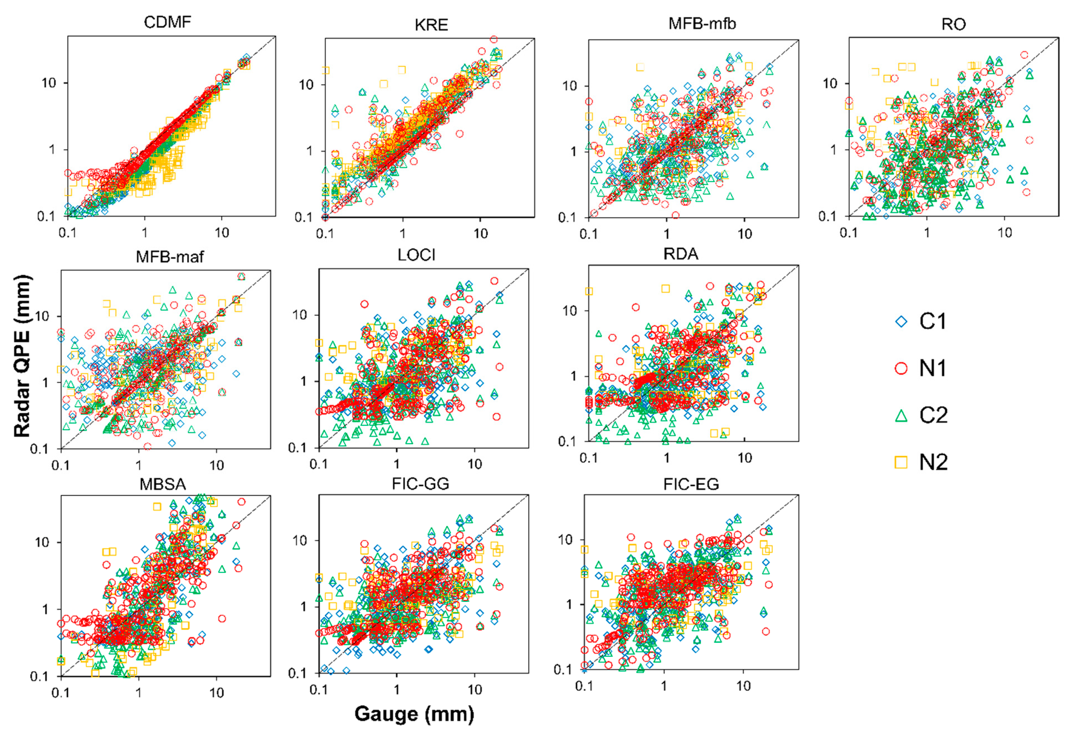
| Radar QPE | Description | Formula | Reference |
|---|---|---|---|
| C1 | Combined Z and KDP algorithm using a threshold on KDP | [79] | |
| C2 | Multi-parameter rain rate estimator using KDP and ZDR | [43] | |
| N1 | NEXRAD Level III (DPA) | [59] | |
| N2 | NEXRAD Level III (OHA) | [59] |
| Event No | Start Date | UTC | End Date | UTC | Season | Duration (Hours) | Max Total Rainfall (mm) | Max Rainfall Intensity (mm/h) |
|---|---|---|---|---|---|---|---|---|
| 1 | 1 June 2012 | 8:00 | 1 June 2012 | 23:00 | Summer | 16 | 39 | 28.0 |
| 2 | 28 May 2013 | 20:00 | 29 May 2013 | 8:00 | Spring | 14 | 60 | 39.2 |
| 3 | 8 July 2013 | 18:00 | 9 July 2013 | 2:00 | Summer | 9 | 93.8 | 46.8 |
| 4 | 31 July 2013 | 19:00 | 1 August 2013 | 10:00 | Summer | 16 | 50 | 17.6 |
| 5 | 28 July 2014 | 0:00 | 28 July 2014 | 12:00 | Summer | 13 | 85 | 81.0 |
| 6 | 6 September 2014 | 0:00 | 6 September 2014 | 10:00 | Fall | 11 | 52.6 | 21.9 |
| 7 | 20 April 2015 | 3:00 | 20 April 2015 | 19:00 | Spring | 17 | 32 | 6.1 |
| 8 | 30 May 2015 | 15:00 | 31 May 2015 | 23:00 | Spring | 33 | 66 | 19.0 |
| 9 | 8 June 2015 | 0:00 | 8 June 2015 | 13:00 | Summer | 14 | 44.2 | 32.0 |
| 10 | 27 June 2015 | 17:00 | 28 June 2015 | 21:00 | Summer | 29 | 57 | 26.0 |
| 11 | 28 October 2015 | 7:00 | 28 October 2015 | 23:00 | Fall | 17 | 49.8 | 11.0 |
| 12 | 10 November 2015 | 19:00 | 11 November 2015 | 11:00 | Fall | 17 | 20.4 | 8.0 |
| 13 | 13 August 2016 | 16:00 | 14 August 2016 | 1:00 | Summer | 11 | 45.2 | 28.8 |
| 14 | 16 August 2016 | 8:00 | 16 August 2016 | 19:00 | Summer | 12 | 34.4 | 12.8 |
| 15 | 23 June 2017 | 5:00 | 23 June 2017 | 14:00 | Summer | 10 | 65.2 | 25.2 |
| 16 | 20 July 2017 | 15:00 | 20 July 2017 | 17:00 | Summer | 3 | 41.6 | 31.4 |
| 17 | 27 July 2017 | 0:00 | 27 July 2017 | 15:00 | Summer | 16 | 15.2 | 7.6 |
| 18 | 18 November 2017 | 22:00 | 19 November 2017 | 8:00 | Fall | 11 | 20 | 11.0 |
| Merging Method | RMSE Decrease (%) | BIAS Decrease (%) | r Increase (%) | |||||||||
| C1 | N1 | C2 | N2 | C1 | N1 | C2 | N2 | C1 | N1 | C2 | N2 | |
| CDFM | 86.94 | 90.50 | 89.41 | 79.85 | 14.86 | 94.72 | 3.76 | 50.01 | 193.83 | 127.50 | 146.43 | 206.89 |
| MFB-mfb | 57.25 | 70.51 | 60.71 | 43.15 | 20.00 | 56.64 | 19.05 | 55.78 | 37.02 | 66.08 | 27.64 | 105.87 |
| MFB-maf | 42.14 | 25.26 | 25.00 | 22.40 | 20.00 | 56.64 | 10.00 | 42.32 | 52.60 | 66.08 | 27.64 | 105.87 |
| RDA | 58.73 | 60.23 | 64.26 | 63.86 | 89.94 | 32.61 | 92.56 | 30.11 | 49.03 | 54.85 | 32.68 | 99.65 |
| LOCI | 57.14 | 66.10 | 60.62 | 53.07 | 40.00 | 62.55 | 19.05 | 76.75 | 52.65 | 66.08 | 27.69 | 105.87 |
| FIC-EG | 77.70 | 79.47 | 78.22 | 66.74 | 96.96 | 10.00 | 94.90 | 61.55 | 62.81 | 51.68 | 39.30 | 94.97 |
| FIC-GG | 68.32 | 79.31 | 68.66 | 59.21 | 89.29 | 41.72 | 91.68 | 13.54 | 55.70 | 49.39 | 30.11 | 98.09 |
| MBSA | 37.11 | 49.48 | 50.00 | 28.57 | 20.00 | 7.09 | 4.76 | 61.55 | 123.40 | 70.70 | 86.48 | 116.85 |
| KRE | 68.14 | 53.23 | 57.50 | 78.31 | 67.90 | 71.42 | 51.23 | 78.85 | 191.87 | 118.66 | 111.11 | 170.57 |
| Merging Method | RMSF Decrease (%) | MAE Decrease (%) | ||||||||||
| C1 | N1 | C2 | N2 | C1 | N1 | C2 | N2 | 1.00 | ||||
| CDFM | 54.46 | 58.52 | 59.94 | 9.78 | 91.06 | 94.17 | 91.98 | 84.23 | 25.00 | |||
| MFB-mfb | 24.71 | 21.22 | 11.58 | 70.32 | 70.61 | 73.28 | 75.36 | 67.04 | 50.00 | |||
| MFB-maf | 30.00 | 11.09 | 44.33 | 77.50 | 3.07 | 46.99 | 35.30 | 72.10 | 75.00 | |||
| RDA | 31.78 | 15.81 | 13.91 | 75.88 | 69.38 | 59.36 | 68.65 | 68.04 | 100.00 | |||
| LOCI | 28.26 | 19.99 | 21.33 | 69.05 | 68.40 | 61.87 | 68.02 | 57.11 | 125.00 | |||
| FIC-EG | 33.13 | 5.45 | 23.60 | 25.80 | 72.21 | 63.59 | 71.31 | 52.23 | 150.00 | |||
| FIC-GG | 40.52 | 16.38 | 31.87 | 73.81 | 71.35 | 63.59 | 70.34 | 69.80 | 200.00 | |||
| MBSA | 3.95 | 17.81 | 3.65 | 65.66 | 43.82 | 8.45 | 45.98 | 33.76 | (%) | |||
| KRE | 52.16 | 18.97 | 44.71 | 63.07 | 76.46 | 61.83 | 55.14 | 78.00 | ||||
© 2020 by the authors. Licensee MDPI, Basel, Switzerland. This article is an open access article distributed under the terms and conditions of the Creative Commons Attribution (CC BY) license (http://creativecommons.org/licenses/by/4.0/).
Share and Cite
Wijayarathne, D.; Coulibaly, P.; Boodoo, S.; Sills, D. Evaluation of Radar-Gauge Merging Techniques to Be Used in Operational Flood Forecasting in Urban Watersheds. Water 2020, 12, 1494. https://doi.org/10.3390/w12051494
Wijayarathne D, Coulibaly P, Boodoo S, Sills D. Evaluation of Radar-Gauge Merging Techniques to Be Used in Operational Flood Forecasting in Urban Watersheds. Water. 2020; 12(5):1494. https://doi.org/10.3390/w12051494
Chicago/Turabian StyleWijayarathne, Dayal, Paulin Coulibaly, Sudesh Boodoo, and David Sills. 2020. "Evaluation of Radar-Gauge Merging Techniques to Be Used in Operational Flood Forecasting in Urban Watersheds" Water 12, no. 5: 1494. https://doi.org/10.3390/w12051494
APA StyleWijayarathne, D., Coulibaly, P., Boodoo, S., & Sills, D. (2020). Evaluation of Radar-Gauge Merging Techniques to Be Used in Operational Flood Forecasting in Urban Watersheds. Water, 12(5), 1494. https://doi.org/10.3390/w12051494