Article

Modeling Daily and Monthly Water Quality Indicators in a Canal Using a Hybrid Wavelet-Based Support Vector Regression Structure

Department of Environmental Science and Engineering, Fudan University, Shanghai 200438, China
*
Author to whom correspondence should be addressed.
Water 2020, 12(5), 1476; https://doi.org/10.3390/w12051476
Submission received: 24 April 2020 / Revised: 30 April 2020 / Accepted: 19 May 2020 / Published: 21 May 2020
(This article belongs to the Special Issue Water-Quality Modeling)

Abstract

:
Accurate prediction of water quality indicators plays an important role in the effective management of water resources. The models which studied limited water quality indicators in natural rivers may give inadequate guidance for managing a canal being used for water diversion. In this study, a hybrid structure (WA-PSO-SVR) based on wavelet analysis (WA) coupled with support vector regression (SVR) and particle swarm optimization (PSO) algorithms was developed to model three water quality indicators, chemical oxygen demand determined by KMnO4 (CODMn), ammonia nitrogen (NH3-N), and dissolved oxygen (DO), in water from the Grand Canal from Beijing to Hangzhou. Modeling was independently conducted over daily and monthly time scales. The results demonstrated that the hybrid WA-PSO-SVR model was able to effectively predict non-linear stationary and non-stationary time series and outperformed two other models (PSO-SVR and a standalone SVR), especially for extreme values prediction. Daily predictions were more accurate than monthly predictions, indicating that the hybrid model was more suitable for short-term predictions in this case. It also demonstrated that using the autocorrelation and partial autocorrelation of time series enabled the construction of appropriate models for water quality prediction. The results contribute to water quality monitoring and better management for water diversion.

1. Introduction

Due to intensified human activities and growth in living standards, many cities around the world are facing challenges of critically deteriorating water quality [1,2]. Water quality is a description of the chemical, physical, and biological characteristics of water with respect to its suitability for intended uses [3,4]. Reliable forecasting of water quality allows for the identification of future contaminant problems, and/or the initiation of effective countermeasures to prevent water pollution and protect public health. In China, the South-to-North Water Diversion Project is a major undertaking designed to resolve water shortage problems in northern China. The east route of the project uses an old artificial canal, known as the Grand Canal, which extends from Beijing to Hangzhou, as a diversion structure. Unlike some natural rivers, this artificial canal is usually characterized by a slow flow rate and irregular changes in water flow, as the canal occasionally opens and closes sluices to transfer a large amount of water. The water quality of the Grand Canal is a critical problem for the water diversion project, and predicting the degree of pollution along the canal is essential to guarantee water quality safety. In the past, a lot of forecasting models have been used in natural rivers, and they performed very well [5,6]. These models usually focused on only dissolved oxygen or the turbidity and salinity of water, but gave less attention to organic pollutants and nutrients pollutants [7,8]. Several previous studies have examined the spatial and temporal variations in water quality along the Grand Canal [9,10]. However, predicting water quality in the canal and this area has been comparatively scarce; even more rare and difficult is forecasting water quality using data with different measurement frequencies.
Many research efforts over the past decade have been aimed at developing and improving water quality prediction models [11,12]. Statistical models of time series data have become particularly popular in water quality [13,14]. A popular and widely used one is the autoregressive integrated moving average (ARIMA) model, which has already shown its capability in water quality prediction [5]. Statistical modeling of water quality possesses many advantages, including simplification of complex of relations between water quality indicators, and the identification of similar temporal and spatial characteristics patterns among water quality indicators [15,16]. However, accurately describing nonlinear characteristics of a data series is a significant shortcoming of the approach, because the statistical models are usually based on temporal linear correlations within the modeled dataset.
To overcome this shortage, machine learning is widely used to address a range of nonlinear prediction problems, recently including the prediction of water quality [17,18,19]. A support vector machine (SVM) is a typical model that represents an advanced form of machine learning and shows remarkable performance. SVM is well-known for its ability to improve classification and regression analysis [20,21]. Using kernel techniques as a part of a time series prediction provides for a more accurate estimation of the data, even where the data series are nonlinear, non-stationary, and not characterized a priori [22]. In the recent years, the particle swarm optimization (PSO) algorithm has been applied to the optimization approach [23]. It is also a good way to optimize model parameters when using SVM models [24].
Currently, hybrid models have been extensively applied in a wide range of fields including environmental pollution forecasting and hydrology [25,26,27]. Wavelet analysis is also a popular recent approach to data analysis and can distinguish between noise and useful signals information. Wavelet analysis is able to capture the non-stationary characteristics of data series and has been applied successfully to forecasting activities [28]. Najah et al. [28] used wavelet analysis and Adaptive Neuro-Fuzzy Inference System to predict the electrical conductivity, the total dissolved solids and turbidity in a river. Liu and colleagues made dissolved oxygen prediction in crab culture based on wavelet analysis and least squares support vector machine [29]. However, there is a lack of studies on other water quality indicators, as well as in the different hydrological environment.
With the important position of the Grand Canal in the water diversion project and the national requirements of monitoring the water quality to guarantee water safety, this study tried to examine the efficiency of a hybrid model in predicting three organic pollutants and nutrients water quality indicators for this manually controlled canal. In this study, a wavelet analysis-support vector regression approach with particle swarm optimization algorithms (WA-PSO-SVR) over different time scales was established. The analyzed data include: (1) daily data collected over a period of one year (1 April 2015 to 1 March 2016), and (2) monthly data obtained over a period of about twelve years (January 2005 to November 2016). Three water quality indicators were modeled, including chemical oxygen demand determined by KMnO4 (CODMn), ammonia nitrogen (NH3-N), and dissolved oxygen (DO). The performance of the models developed for both time scales were compared and assessed. In addition, to assess the potential advantages of using the WA-PSO-SVR model, its results were compared to the results from a simple support vector regression with particle swarm optimization model (PSO-SVR) and a standalone SVR model, which were developed for the datasets.
This research demonstrates the reliability and suitability of the hybrid model in forecasting water quality indicators in situations. The results are helpful for (1) providing an effective method of water quality prediction for water diversion in the region towards better governance policies in daily management, (2) adding more research materials for the hybrid model applied in different water quality indicators and hydrological environment, and (3) contributing to the fields of non-linear water quality data prediction modeling over different time scales.

2. Materials and Methods

2.1. Study Area and Data Used

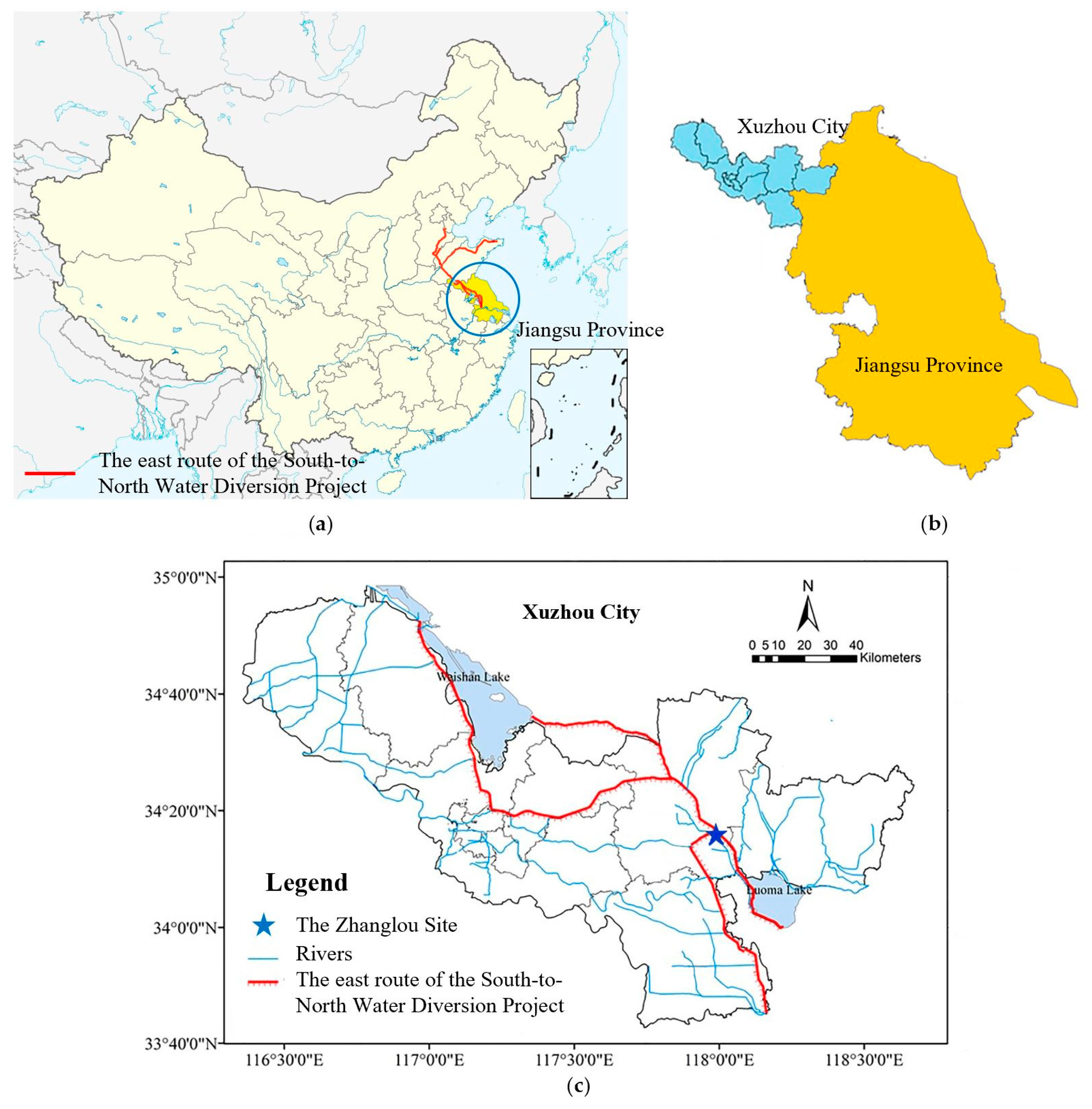
Xuzhou City is located in Jiangsu Province, China, and is one of the cities positioned along the east route of the South-to-North Water Diversion Project. The first stage of the east route project was constructed from 2005 to 2013, and water transmission started from the end of 2013. To ensure the water quality safety requirements of water diversion, six state-controlled water quality monitor sites (i.e., Zhanglou, Linjiaba, Shanjizha, Shazhuangqiao, Lijiqiao, and Shajixizha) were established in Xuzhou. Since 2013, five auto-monitoring systems at these monitor sites (except Shanjizha) were set up successively. The Zhanglou sampling site (34°15′58″ N, 117°59′33″ W), where the data for this study were collected, is located within the Huai River basin along the main channel of the Grand Canal, which extends from Beijing to Hangzhou (Figure 1).
Water quality data from rivers often exhibit periodicity, which is commonly related to annual or seasonal variations in system hydrology and environmental conditions. The most recent research has considered only a single time scale. For example, Kisi and Parmar [30] compared three models using ten years of monthly COD data. Another nearly twenty-year monthly dataset was studied by Barzegar and colleagues [31,32]. In this study, the performance of predictive models over different time scales was analyzed to obtain a better understanding of their predictive capabilities. These models independently used daily and monthly water quality data collected from the Zhanglou monitoring site. The daily data consisted of a total of 366 auto-monitoring datasets obtained from 1 April 2015 to 31 March 2016 from the auto-monitoring system. The monthly data included 143 records that were based on manually collected monitoring data obtained from January 2005 to November 2016. These data were collected by the Xuzhou Environmental Monitoring Centre. Previous research has shown that the water quality in the Xuzhou area was influenced strongly by industrial and urban activities; nutrient concentrations in the water body are particularly high [10]. For example, because Xuzhou is a mining city, it possesses several mining and metallurgical industries. In addition, Xuzhou, with a population of 10.29 million (up to 2015), has long supported agriculture. Given the high concentrations of organic pollutants and nutrients, three indicators, i.e., chemical oxygen demand determined by KMnO4 (CODMn), ammonia nitrogen (NH3-N), and dissolved oxygen (DO), were selected for analysis. These parameters were selected because (1) they provide a general overview of the degree to which organic pollutants and nutrients have contaminated the river, and (2) the measurement and control of these pollutants is one of the primary tasks inherent in the operation of the water diversion [33,34]. Thus, CODMn, NH3-N, and DO were selected as the target indicators used to develop and test the predictive models in this study. A statistical summary of these three water quality indicators for both daily and monthly time scales is presented in Table 1. Table 1 also includes information on whether the time series are stationary. Water was not transferred daily or on a regular pattern. Rather, transfers depended on the demand for water in northern areas, which were usually conducted in winter or spring. As a result, the water flows tended to significantly change on transferring days. With regards to the monthly data series, significant efforts to control waste water and non-point source pollution led to a slight decrease in the pollution level within the region.
For the generation of the daily model, the first 305 sets of auto-monitoring data were used for model training. The remaining 61 sets of data were used to evaluate the performance of the established models. Generation of the monthly model used 119 sets of manually collected monitoring data for training, and 24 sets of data for testing. The basic methods used in this study are described below.

2.2. Wavelet Analysis (WA)

Wavelet transforms are efficient for data analysis, picture and signal processing, resolution reconstruction, and information detection [35,36]. They have been shown to be a useful and powerful mathematical tool for the analysis and processing of non-stationary time series [37,38]. While the wavelet transform theory is similar to the Fourier transform, wavelet transforms allow the signal to be dilated and translated, and time-frequency features can be extracted through a completely flexible window function called the mother wavelet [39]. Continuous wavelet transform (CWT) is a formal tool that provides an overcomplete representation of a signal x(t) by letting the translation and scale parameter of the wavelets vary continuously. The wavelet is defined as:
W ( τ ,   a ) = 1 a x ( t ) Ψ   ( t τ a ) d t
where Ψ ( t ) represents a continuous function in both the time domain and the frequency domain called the mother wavelet, a is the scale or frequency factor, and τ is the time shifting factor.
The discrete wavelet transform is more commonly used than the successive wavelet transform, due to its lower computational time requirements and simpler development process [40]. Based on the decomposition of the original signal into different signal channels at various levels, a discrete wavelet transform (DWT) can be derived from a CWT by expanding the orthogonal basis of scaling and wavelet functions. The signal x(t) can be represented by scaling coefficients m 0 k and wavelet coefficients n j k :
x ( t ) = k = m 0 k φ j k ( t ) + j = 1 k = n j k Ψ j k ( t )
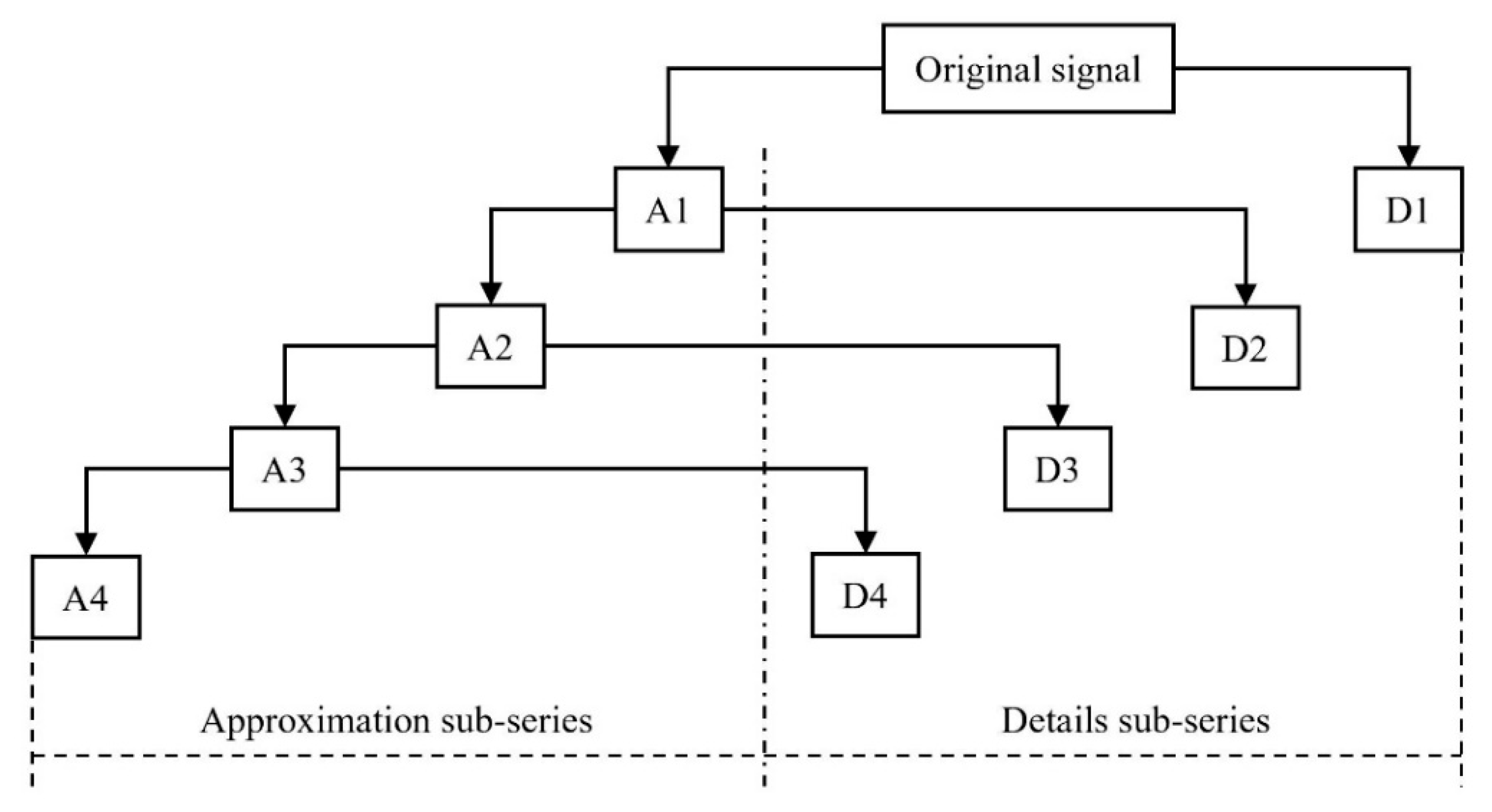
DWT uses both a high-pass and a low-pass filter to separate the frequency-bands of the signal. The structure of a four-layer multi-resolution analysis is illustrated in Figure 2 after decomposition. The high-pass filter g(t) produces several sets of detail coefficients, c D j , which are associated with the wavelet function, while the low-pass filter h(t) produces the approximation coefficients, c A j , which are associated with the scaling function (Figure 2). These coefficients can be represented as:
c A j + 1 ( t ) = h ( n 2 t ) c A j ( n )
c D j + 1 ( t ) = g ( n 2 t ) c A j ( n )
where n is the number of samples and j is the last decomposition level.

2.3. Support Vector Regression (SVR)

The support vector machine (SVM) proposed by Vapnik [41,42] is a supervised learning model that analyses data used for classification and regression analysis. Based on the principle of structured risk minimization, SVM uses a suitable kernel function to construct an optimal separating hyperplane, which simultaneously maximizes the geometric margin and minimizes the upper bound of the generalization error, instead of the empirical error [43]. Additionally, SVM is extended to solve regression problems by applying a set of high dimensional linear functions. The regression function of an SVM (SVR) can be formulated as follows:
d = w T x + b
where w is the weight vector, b is the bias, and d and x belong to the training sample J = { x i , d i } i = 1 N . With the introduction of an ε-insensitive loss function, the coefficients w and b are estimated by minimizing the risk functional:
1 2 w 2 + C i = 1 N | y i d i | ε
which is subjected to the following constraints (Equations (7)–(10)): for i = 1 ,   2 , , N
d i y i ε + ξ i
y i d i ε + ξ i
ξ i 0
ξ i 0
In (Equation (6)), C is a constant that determines the trade-off between the training error and the penalization term w 2 , and y i is the estimator output. The ξ i and ξ i (Equations (9) and (10)) are two sets of nonnegative slack variables. To solve this optimization problem, Lagrange multipliers are introduced, and the minimization formula can be expressed as follows:
J ( w , ξ , ξ i , α , α , γ , γ ) = 1 2 w 2 + C i = 1 N ( ξ i + ξ i ) i = 1 N ( γ i ξ i + γ i ξ i ) i = 1 N α i ( w T x i + b d i + ε + ξ i ) i = 1 N α i ( d i w T x i b + ε + ξ i ) α , α , γ , γ 0 ,   i = 1 , 2 , , N
where α i and α i are the Lagrange multipliers. Then, by calculating the partial derivatives of w , b, ξ and ξ , and setting the resulting derivatives equal to zero, the original problem can be conversed to its dual problem. Finally, the SVR can be expressed as:
f ( x ) = i = 1 N ( α i α i ) ( x i , x ) + b
In order to convert a problem to a nonlinear regression problem, a kernel function was introduced. There are four suggested possible choices for the kernel function, namely linear, polynomial, radial Gaussian, and sigmoid. Using K ( x i , x ) instead of ( x i , x ) , the nonlinear SVR function can be presented as follows:
f ( x ) = i = 1 N ( α i α i ) K ( x i , x ) + b
During the SVR modeling process, the radial basis function (RBF) kernel was selected. As a kernel function, it is a good default kernel and is widely used [44]. Two parameters, the penalty factor c and the parameter gamma g in the RBF kernel, are important and need to be chosen by users. As for the parameter c, if it is too large, the model may have a high penalty for non-separable points and overfit; conversely, if too small, it would be underfit [45]. Gamma g is a free parameter of RBF, and a large g means a Gaussian distribution with a small variance, implying the support vector does not have wide-spread influence, which therefore leads to high bias and low variance models (and vice versa). In practice, the parameters c and g were varied through a wide range of scales. Therefore, the PSO method was introduced to optimize these parameters for the SVR models, as described below.

2.4. Particle Swarm Optimization (PSO) Algorithms

The PSO algorithm is an optimization algorithm for improving candidate solutions that simulate the movement of social behavior [46]. The technique includes a population of proposed solutions or particles moving toward the optimal solution of the problem; a new population is obtained that shifts the position of the previous population during each iteration.
The “particle” of the swarm X i represents its position in the search space of possible solutions. The particle position X i 0 and its velocity V i 0 can be obtained randomly and then adjusted dynamically according to its historical behavior. The optimal local location of the particle is p l , whereas p g is the optimum solution searched by the particle in the global space.
The basic mathematical expressions for PSO are as follows:
v i j ( t + 1 ) = v i j ( t ) + c 1 r 1 ( p l j ( t ) x i j ( t ) ) + c 2 r 2 ( p g j ( t ) x i j ( t ) )
x i j ( t + 1 ) = x i j ( t ) + v i j ( t + 1 )
where t is the iteration number, r 1 and r 2 are random variables obeying a uniform distribution of the interval (0, 1), and c 1 and c 2 are acceleration constants.
The PSO algorithm guides particles to search for the optimal solution through individual competition and cooperation among the community. An inertia weight w is introduced to control the optimization performance. If ζ = ζ 1 + ζ 2 , where ζ 1 = c 1 r 1 and ζ 2 = c 2 r 2 , the equations can be represented as:
v ( t + 1 ) = w v ( t ) + ζ ( s x ( t ) )
x ( t + 1 ) = x ( t ) + v ( t + 1 )
where s = ζ 1 p l + ζ 2 p g ζ 1 + ζ 2 . The velocity recurrence relation at time t, t + 1, t + 2 is:
v ( t + 2 ) + ( ξ 1 w ) v ( t + 1 ) + w v ( t ) = 0

2.5. Model Development

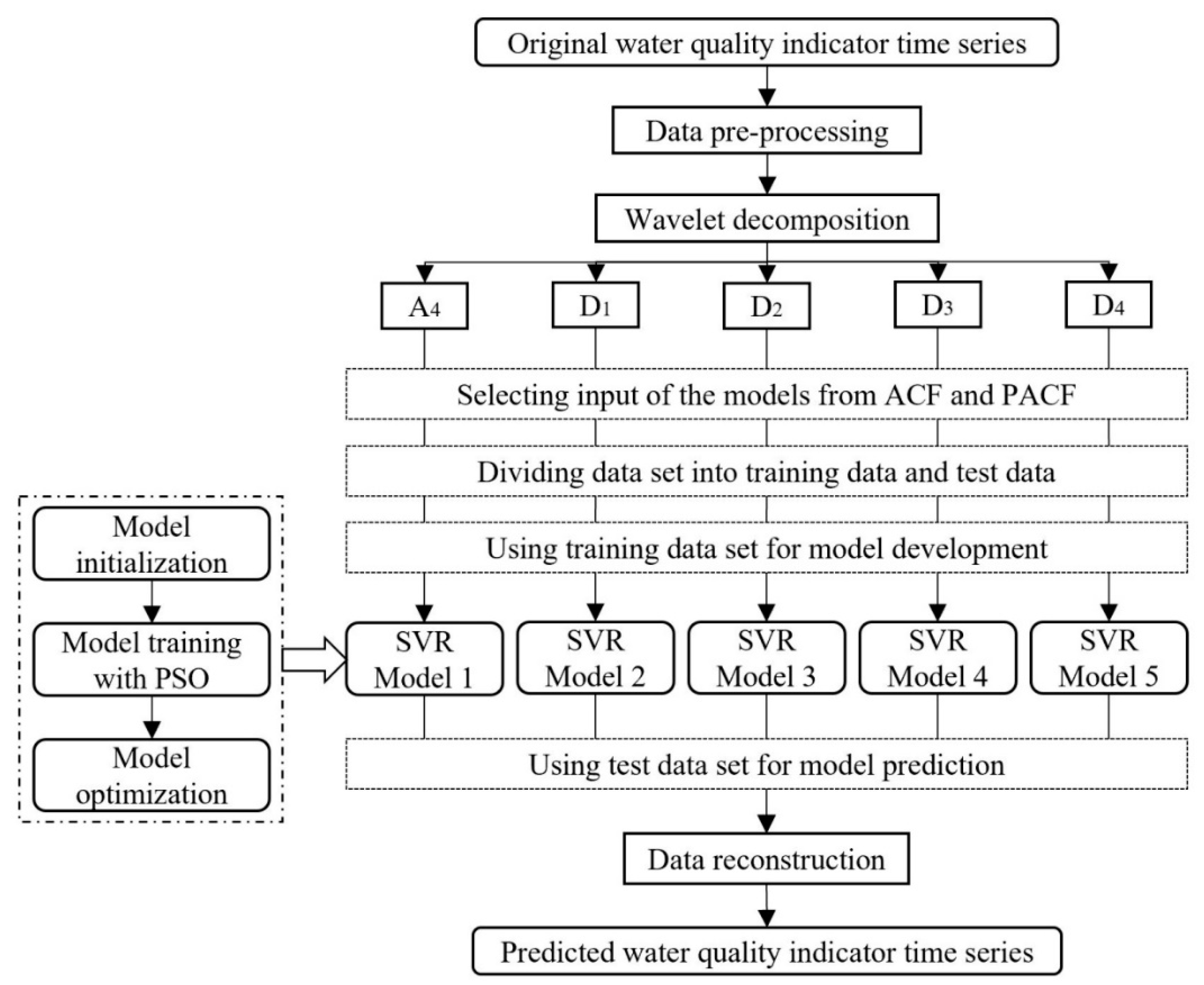
The wavelet analysis and SVR models have a unique advantage in capturing both linear and nonlinear data characteristics. Thus, in this study, WA, SVR, and PSO components were constructed together as a hybrid model to predict CODMn, NH3-N, and DO at the selected monitoring site. The implemented steps used to predict the water quality indicators are shown in Figure 3 and included the following:
  • Data pre-processing. Due to occasional inefficiencies of the auto-monitoring systems, some auto-monitoring data were missing or erroneous. Thus, statistical outliers and structural zeros were removed from the dataset. In the case of missing data, an exponential smoothing method was used to estimate and replace the missing values.
  • Wavelet analysis. Wavelet analysis was used to decompose each time series into wavelet sub-series. The choice of mother wavelets influences sub-series decomposition and construction. Three mother wavelets that are commonly employed are the Daubechies, Symlet, and Haar. The db3 wavelet is a function based on Daubechies extremal phase wavelets with a vanishing moment of 3; it has often been successfully applied in water quality predictions [29,32]. Thus, a db3 wavelet based on four layers was used herein for decomposing the water quality data series. All the analyzed time series were found to possess five sub-series, one represents the approximation series A4, and the other four are the detailed series from each layer, D1, D2, D3, and D4.
  • Data standardization. In order to remove dimensional effects which may bias the predictive models, the data were standardized by scaling the input variables over their range of observation prior to the modeling processes. The general formula for standardization is:
    x i = x i x m i n x m a x x m i n
    where x i and x i express the normalized and raw observations of variable x, respectively; and x m i n and x m a x refer to the minimum and maximum values of variable x, respectively. Based on the characteristics of the different series and performance of the predictive models, the original data series and approximation series ranged from 0 to 1, while the detail series were between −1 and 1.
  • PSO-SVR modeling. The hybrid model exhibits a multi-input single output structure. The relevant and important input variables in the models were extracted using values from an autocorrelation function (ACF) and partial autocorrelation function (PACF) from each time series, with the criterion of the correlation coefficient set at the 95% confidence level. The PSO method was then applied to deduce the optimal parameter values for the SVR models. For each data series, five predictive models (one model for A4 and four models for D1 to D4) were run and calculated separately.
  • Data reconstruction. After calculation, algebraic sums of the predicted values based on the five sub-series (A4, D1, D2, D3, and D4) were obtained to generate the final forecasting results for each data series.
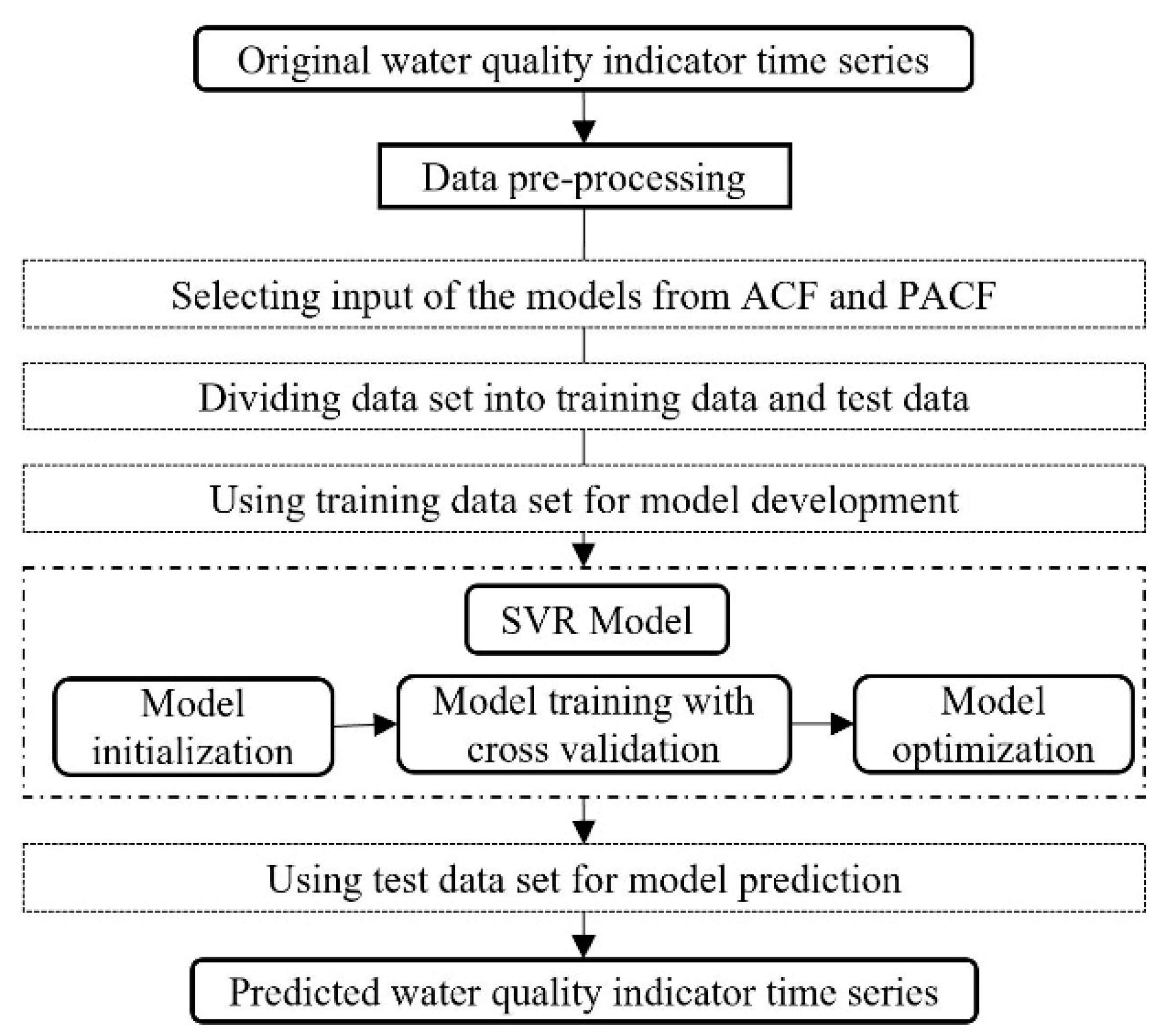
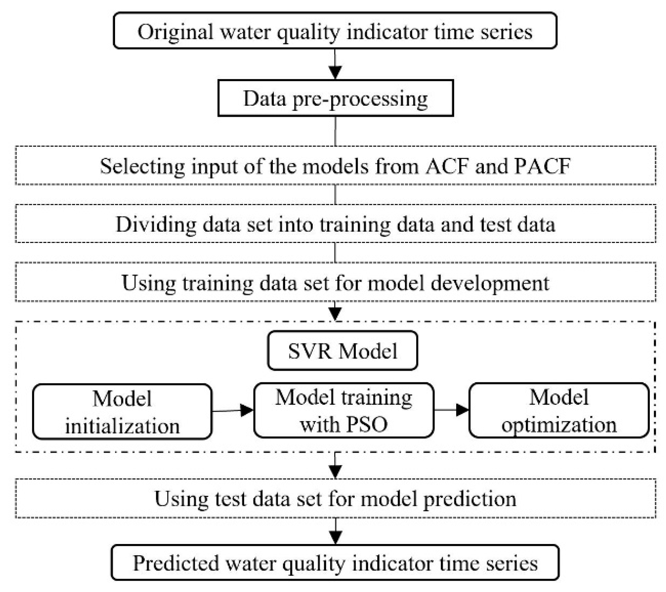
In order to validate the performance of the proposed hybrid model, two other models were developed. One was a standalone SVR model, which refers to developing SVR models of original standardized data series and using basic cross validation to select the optimal model parameters (Appendix A, Figure A1). The other model was a PSO-SVR model, which is similar to the SVR model, but it uses PSO algorithms as the optimization method (Appendix A, Figure A2).

2.6. Performance Assessment of the Models

The performance of the predictive models was evaluated by using four statistical indicators: the root mean square error (RMSE), the mean absolute percentage error (MAPE), the coefficient of determination (R2), and the Nash–Sutcliffe efficiency coefficient (NSE).
Higher R2 and lower RMSE and MAPE values indicate a more precise model. The Nash–Sutcliffe efficiency coefficient (NSE), which ranges from −∞ to 1, can be used to assess the forecasting power of hydrological models [47]. The closer the NSE model efficiency is to 1, the more accurate the model. When NSE = 0, model predictions are as accurate as the mean of the observed data. In contrast, when NSE < 0, the residual variance is larger than the observed data variance and the model is unreliable. Equations (20)–(23) are the mathematical expressions used to calculate RMSE, MAPE, R2, and NSE, respectively:
RMSE = 1 N I = 1 N ( y i ^ y i ) 2
MAPE = I = 1 N | y i ^ y i y i | × 100 %
R 2 = ( i = 1 N ( y i y ¯ ) ( y i ^ y ˜ ) ) 2 i = 1 N ( y i y ¯ ) 2 · i = 1 N ( y i ^ y ˜ ) 2
NSE = 1 i = 1 N ( y i y i ^ ) 2 i = 1 N ( y i y ¯ ) 2
where N is the total number of data points being modeled, y i ^ is the predicted value, y i is the observed value, and y ˜ and y ¯ are the average of predicted and observed values, respectively.

3. Results

This study employed a hybrid forecasting model based on wavelet analysis and SVR with PSO algorithms for optimization to predict three water quality indicators at the Zhanglou monitoring site along the Grand Canal. To assess the predictive ability of the hybrid model, both non-stationary and stationary data series over two-time scales, daily and monthly, were considered. Based on the structure of the hybrid model, all-time series were initially decomposed. Then, the selected input data were used to train the established models and make predictions. Results related to each model are presented below.

3.1. Models for Daily Prediction

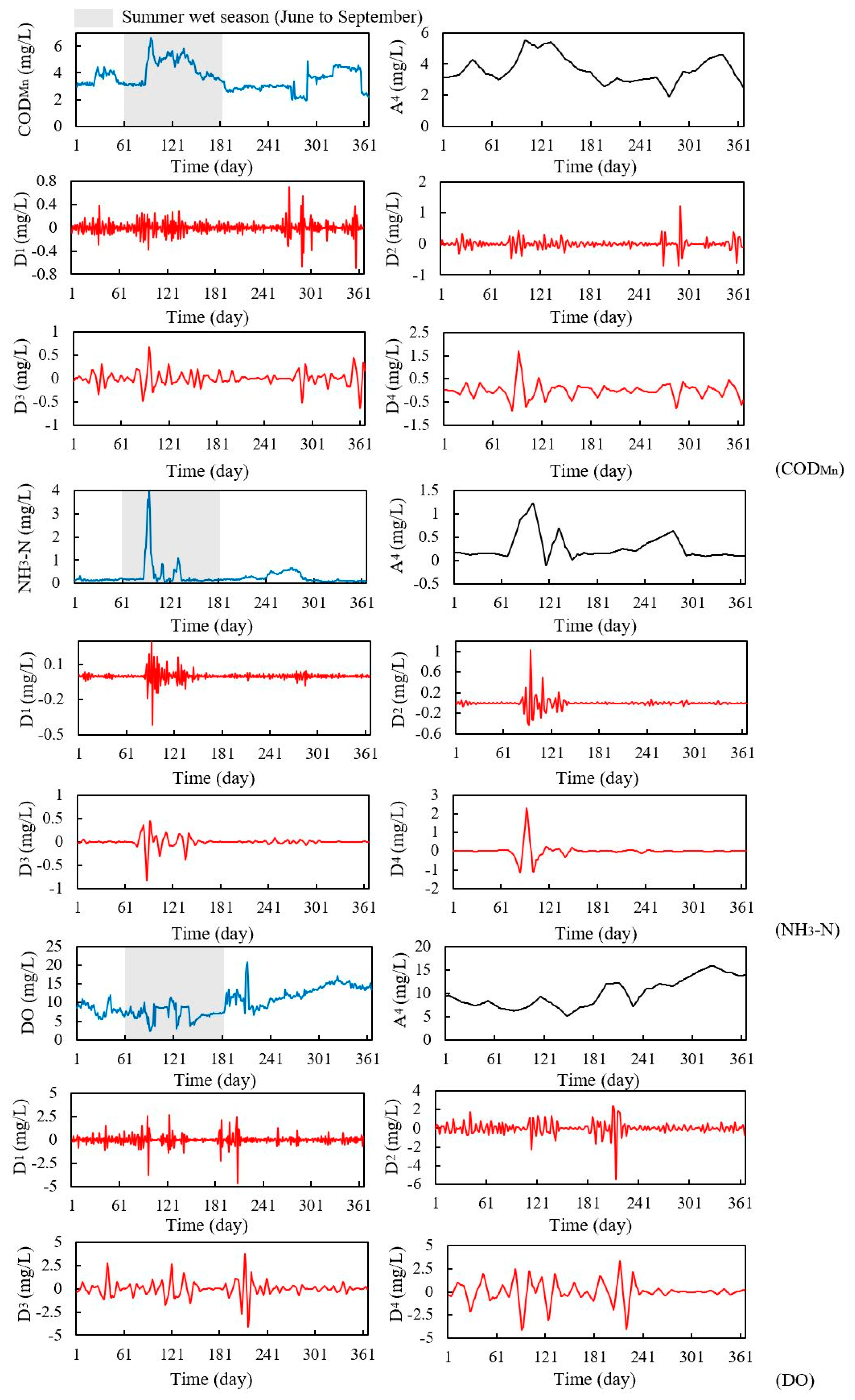
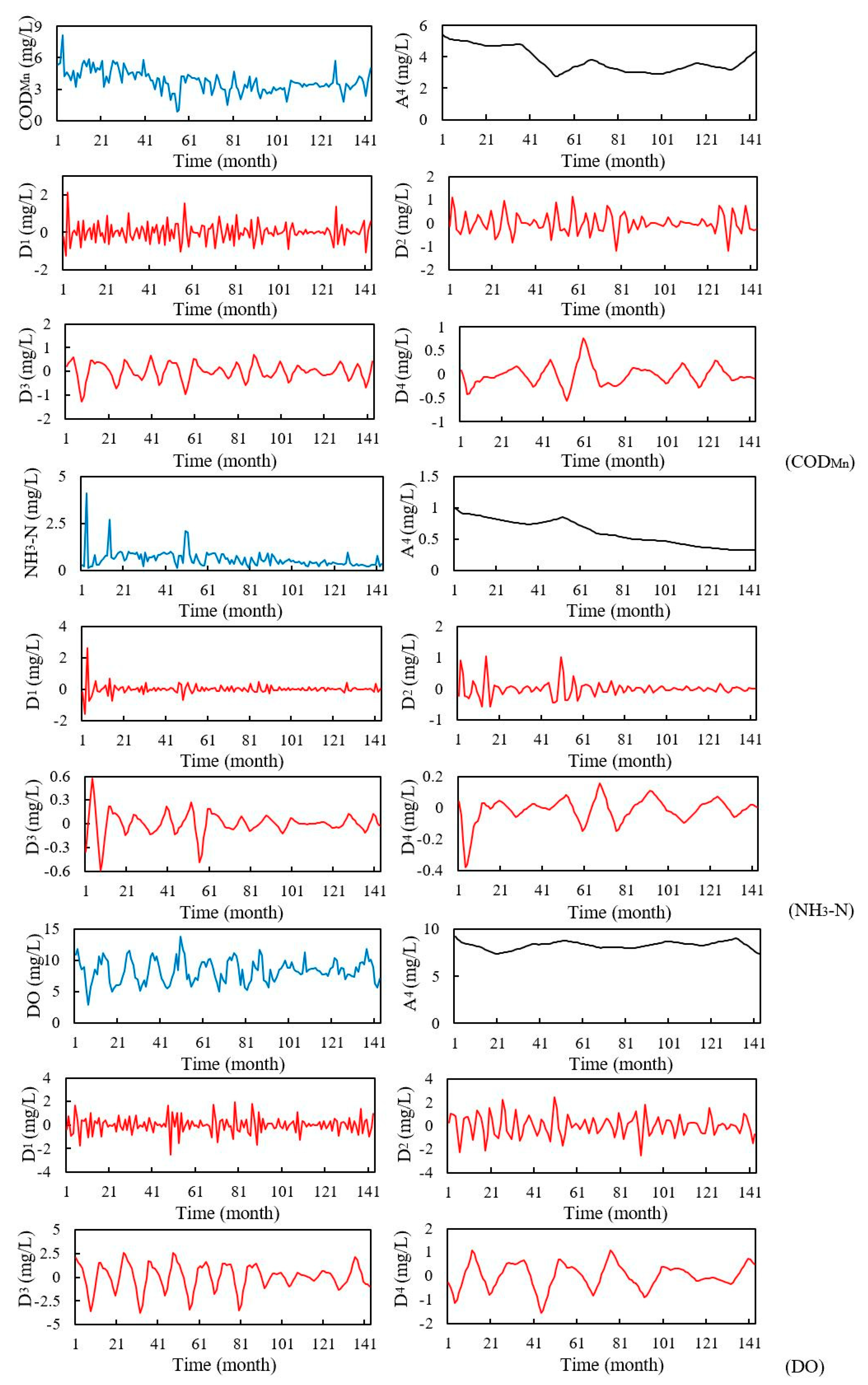
The daily time series of CODMn, NH3-N, and DO were decomposed using the db3 wavelet based on four layers (as described above). The sub-series after decomposition and reconstruction are shown in Figure 4. These three series were all non-linear. All three parameters exhibited considerable fluctuations during the summer wet season (from June to September) (Figure 4). This may be caused by a large amount of precipitation during this period which accounted for more than 80% of the annual precipitation.
Of the three original daily time series, NH3-N was stationary, while CODMn and DO were non-stationary. The decomposed and reconstructed sub-series included both stationary and non-stationary series. For the stationary series, the inputs for subsequent models were selected using their autocorrelation coefficients. For non-stationary series, the inputs were selected by their partial autocorrelation coefficients to obtain a high level of model performance [7]. Results related to the three water quality indicators that were produced by the hybrid WA-PSO-SVR model and the two other contrasting models (i.e., the PSO-SVR and the standalone SVR which used cross validation as optimization method) are presented in Figure 5.
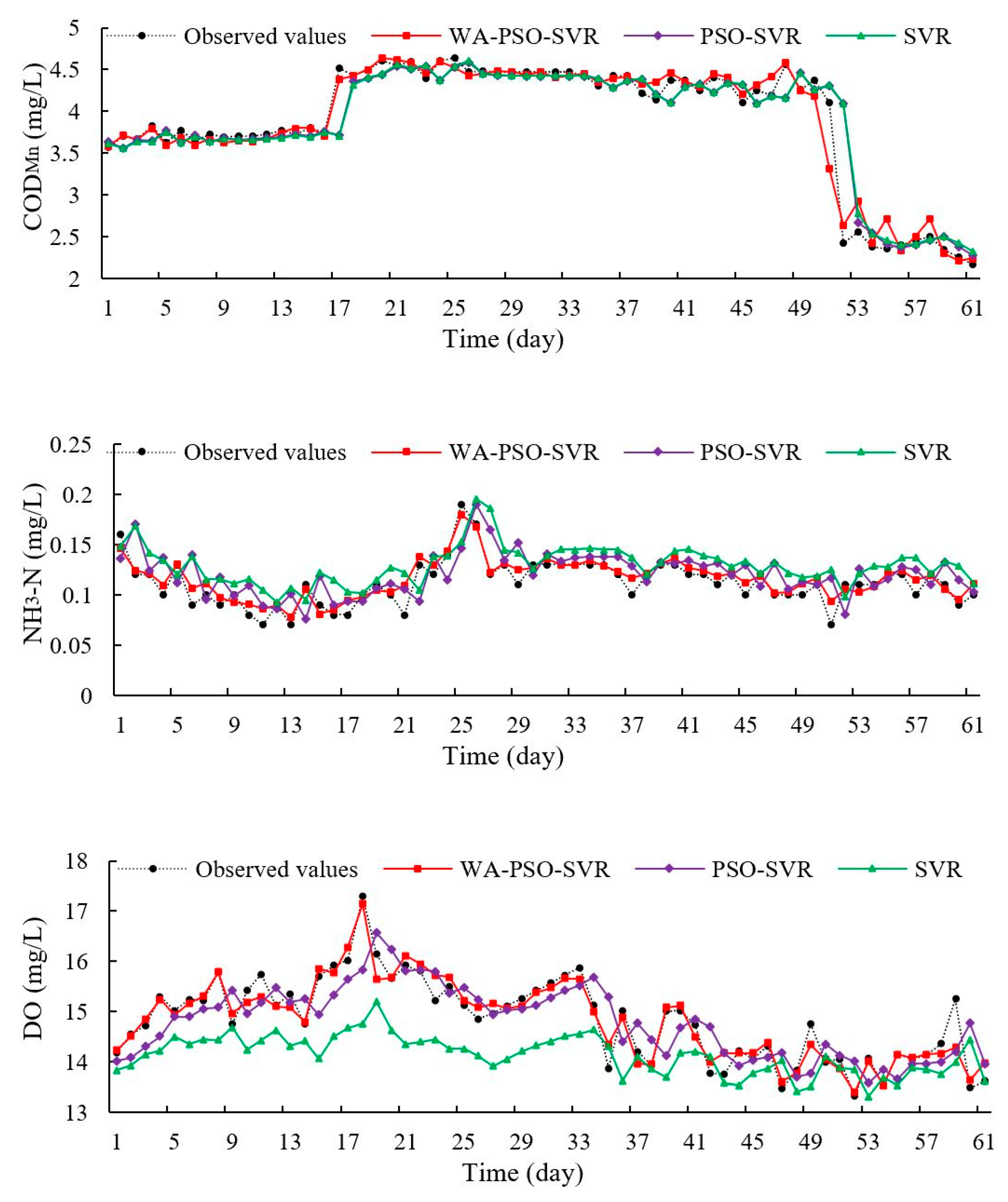
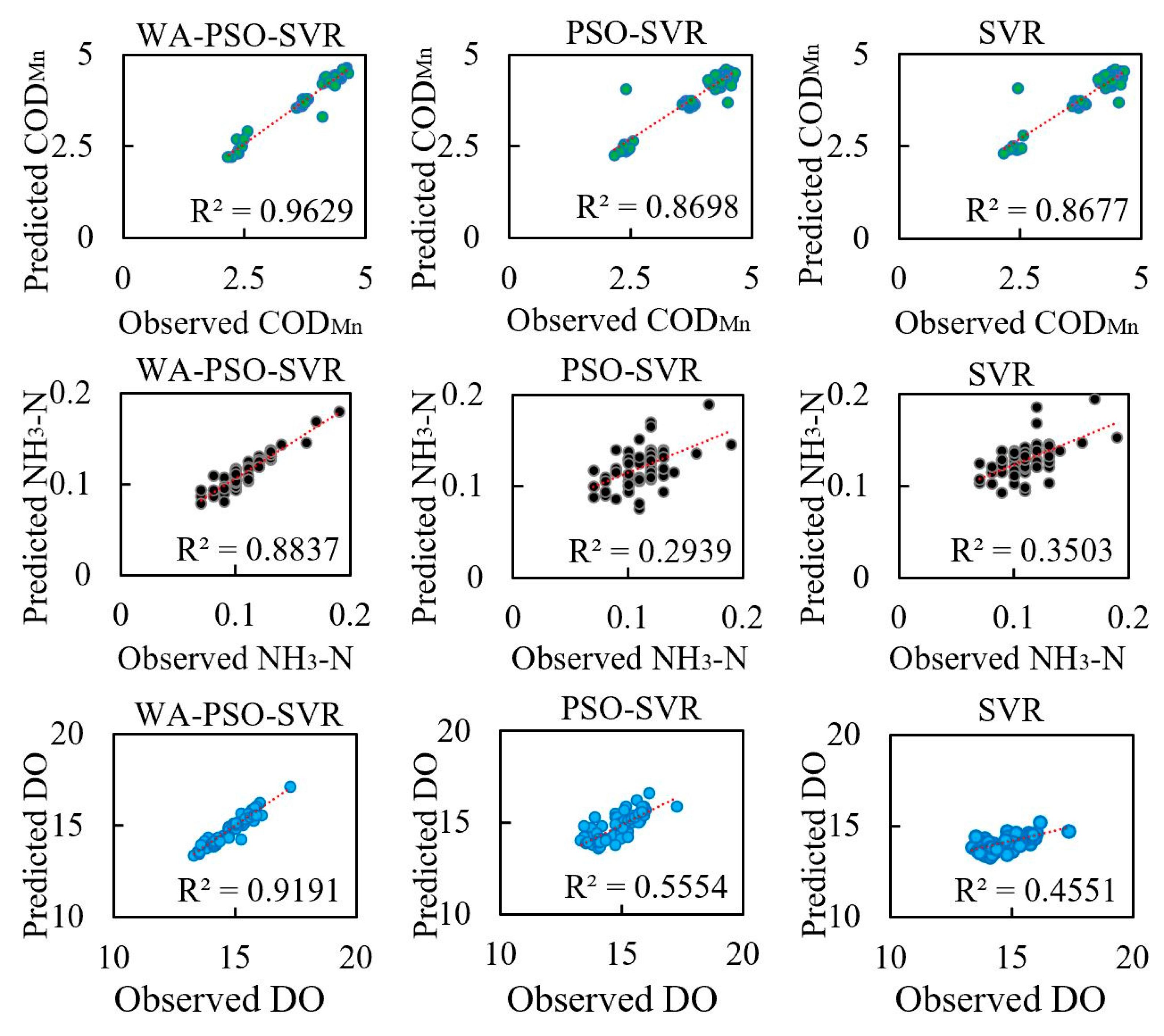
All of the three models predicted changes in trend and performed well as a whole (Figure 5). The prediction of CODMn was better than for the other two indicators (NH3-N and DO). Each indicator was more closely predicted by the WA-PSO-SVR model than by either the PSO-SVR or the single SVR model, especially for the prediction of extreme values. Predictive results generated by the PSO-SVR and the single SVR models were similar; in fact, the results nearly overlap for CODMn. The predication of DO differed significantly among the three models. The performance of the standalone SVR model was lower than that of the other two models when predicted and observed values are compared. In addition, both the PSO-SVR and single SVR models possessed a one-day lag between observed and predicted values, which led to larger model errors that can be seen in scatter plots (Figure 6). The coefficient of determination (R2) for the WA-PSO-SVR models are about 0.9, while the values for the other models are much lower. Although the prediction of DO was the worst (Figure 5), the R2 values of predicting NH3-N were the lowest among the three indicators. The highest R2 value for NH3-N was only 0.8837; it was calculated using the WA-PSO-SVR model. The PSO-SVR model possessed larger errors than the standalone SVR model.
Table 2 provides the statistical evaluation of daily CODMn by the three models. All three models were efficient, with NSE values close to 1. During the testing period, NSE values for the WA-PSO-SVR model were 10.73% and 11.04% higher than the PSO-SVR and standalone SVR model, respectively. RMSE was calculated to be 46.76% and 47.23% lower, while MAPE was 40.77% and 42.86% lower, respectively.
For the prediction of NH3-N (Table 3), the WA-PSO-SVR model performed well, while the other two models had poor performances and were unreliable as they exhibited NSE values below 0. These results illustrate that the hybrid model was the only one that can be used for daily NH3-N prediction.
Table 4 shows that while RMSE and MAPE values are not high, the standalone SVR model was unreliable. However, the WA-PSO-SVR model performed well, and the results possessed the highest NSE value, exceeding 0.9. Compared with the PSO-SVR model, the hybrid model performed 58.16%, 63.87%, and 77.10% better, in terms of RMSE, MAPE, and NSE, respectively.

3.2. Models for Monthly Prediction

As done for daily predictions, the monthly time series of CODMn, NH3-N, and DO were initially decomposed (Figure 7). NH3-N exhibited a declining trend, whereas CODMn and DO exhibited constant trends with generally consistent fluctuations.
Given that the time series data for all three parameters were collected over a nearly twelve-year period, the data possessed periodicity. In the case of DO, the periodicity was on a one-year cycle, presumably because DO was correlated to seasonal water temperatures. Based on unit root testing of the data during pre-processing, NH3-N and DO were found to be non-stationary series, whereas the CODMn series was stationary. Following the selection of inputs for predictive models of each sub-series, the estimated results of the three models were calculated (Figure 8).
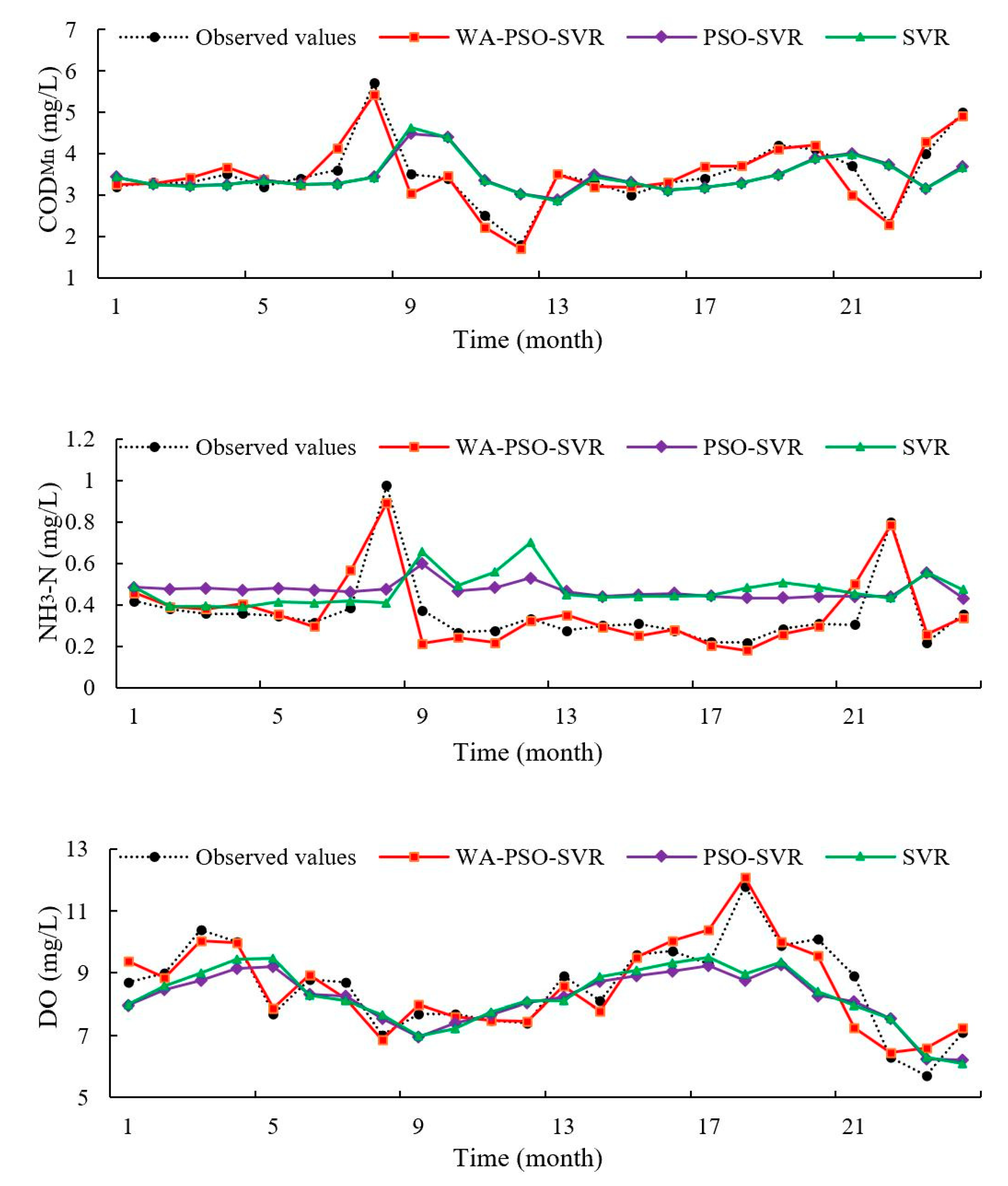
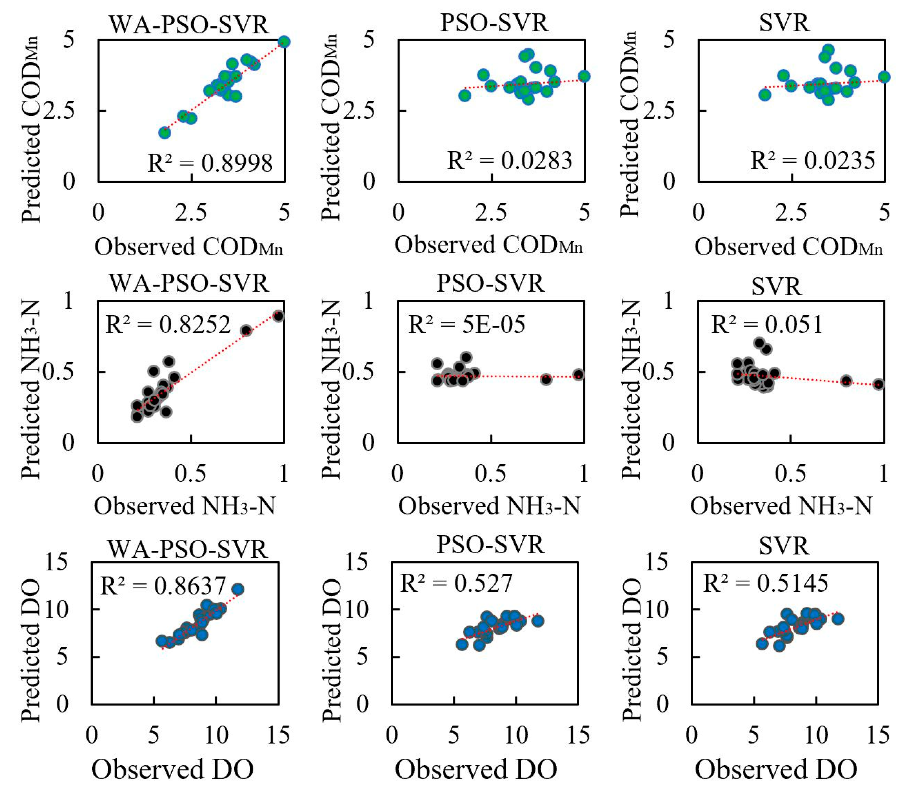
The performances of monthly predictions exhibited some similar characteristics to the daily predictions. The WA-PSO-SVR models of all three indicators performed much better than the other two models. However, in contrast to the daily predictions, the prediction of DO was relatively satisfactory over the monthly time-scale. The prediction of NH3-N exhibited the largest errors. The predicted curves by the PSO-SVR and standalone SVR models for CODMn overlapped (as they did for the daily predictions); the predictions of DO were also similar. The hybrid models were also better at predicting extreme values. This was especially true for the prediction of maximum DO concentrations; the hybrid model was the only one that accurately (closely) described changes in DO. The other two models even predicted values that were opposite to the observed values. In addition, these two models produced predictions that possessed a one-month lag delay in predicted indicators. The scatter plots in Figure 9 show that the WA-PSO-SVR models significantly outperformed the others. The prediction of NH3-N was the worst; the highest R2 value was 0.8252. The prediction of NH3-N also exhibited the largest differences between the hybrid model and the others. The PSO-SVR and standalone SVR models both preformed extremely poorly in terms of NH3-N predictions.
Comparison of observed and predicted CODMn data by the WA-PSO-SVR model during the testing phase produced RMSE, MAPE, and NSE values of 0.2506, 5.126%, and 0.8941, respectively (Table 5). These statistical values show that the model was able to make relatively accurate predictions of monthly CODMn time series. In contrast, the PSO-SVR and SVR models had similar statistical assessment values, with NSE values below 0, indicating they generated undesired predictive results.
The prediction of monthly NH3-N data was similar to CODMn (Table 6). Only the WA-PSO-SVR model produced reliable results, although its MAPE value was much larger for NH3-N than for the prediction of CODMn. RMSE, MAPE, and NSEs values calculated for the results of the other two models illustrate that they all produced large errors and had difficulties in generating satisfactory and accurate results.
All three models were better able to predict NH3-N than the other parameters; the WA-PSO-SVR model outperformed the other two models (Table 7). The WA-PSO-SVR model produced RMSE values that were 50.23% and 48.96% lower in comparison to the results generated by the PSO-SVR and SVR models, respectively. The MAPE values were 55.94% and 56.65% better, respectively, while the NSE values of the WA-PSO-SVR model improved by 99.93% and 87.69% over the others, respectively.

4. Discussion

Because of the requirement of daily water transfer management, an available forecasting model is essential to environmental governance. This model is mainly established for general changing trend prediction helping long-term water pollution control, but not for giving accurate forecasting of emergency or sudden changes caused by accident events, such as flooding or pollution leaks.
Regardless of whether daily or monthly time series data were predicted, the WA-PSO-SVR models produced more accurate results for the three analyzed water quality indicators. The hybrid modeling approach demonstrated to be a reliable approach for water quality prediction. Besides the similar studies that have been done for DO in the river and pond or the turbidity and salinity of water [7,8,29], this study showed that the hybrid structure could be applied in more fields. During this study, the performance of the WA-PSO-SVR models was better when modeling daily data than monthly data, indicating that wavelet analysis, when applied to short-term forecasting, would produce more accurate results. Previous studies led to similar conclusions in that hourly machine learning models outperformed daily models when making DO predictions using wavelet-neural network models [26].
As mentioned above, of the six time series related to the three water quality indicators, only the daily NH3-N and monthly CODMn series were stationary. However, the accuracy of the WA-PSO-SVR modeling results was uncorrelated to whether the time series were stationary. For daily NH3-N and monthly CODMn prediction, the hybrid models generated satisfying results, whereas both the PSO-SVR and SVR produced unreliable results for them, as determined by negative NSE values. The PSO-SVR and SVR have given satisfactory performances in some other studies [21]; however, these results showed a possibility that the hybrid model was more suitable for stationary data than the PSO-SVR and SVR models in this situation. Similar to the stationarity of the data series, when comparing the WA-PSO-SVR and other two models, the model performances were also unrelated to the distribution of data. Wavelet analysis could increase the accuracy of prediction, which was independent of Skewness and Kurtosis values.
The PSO-SVR and SVR curves of observed and predicted values showed that there was a one-step lag in predicted values (Figure 5 and Figure 8). However, these models could effectively re-create changes in parameter trends relatively accurately. This phenomenon has occurred in some studies [7,26]. Usually, it means that the models had some drawbacks and deficient ability to provide accurate extreme values. This may be caused by a lack of sufficient input information by considering only autocorrelation of data series. A good way to solve this deficiency is by using a hybrid decomposition structure [7,27]. In this study, the hybrid WA-PSO-SVR models demonstrated their ability to predict extreme values through time.
Moreover, regardless of the time scale modeled (i.e., daily or monthly data), the estimation of CODMn was extremely good with the highest NSE values, followed closely by DO, and NH3-N was the worst. However, when comparing the RMSE and MAPE values, the results were different. NH3-N had the lowest RMSE, but DO had the lowest MAPE. In general, the prediction of NH3-N was more difficult. The NH3-N models always had larger MAPE and lower NSE among three indicators. This is related to the distribution of the data series. Although all of the original six data series did not have a normal distribution, two NH3-N series had larger absolute values of Skewness and Kurtosis among them, indicating that they were far from normal distribution than other series. Highly skewed and imbalanced data is a reason that could lead to the poor performance of these models [48].
Because there are many indicators that can be used to assess the level of water quality pollution, the prediction of water quality may rely on either multiple and single variable models. However, multivariable models do not always perform better than single variable models because of strong statistical autocorrelations of the water quality indicators [6]. In this study, all models were developed based on their autocorrelation, including models of sub-series decomposed from wavelet analysis. The WA-PSO-SVR modeling results illustrate that these simple models with a single variable had the ability to provide reliable and accurate predictive outcomes. However, previous research has found that models that do not consider autocorrelation can also produce good estimations [19]. Thus, the cross-correlation between indicators or the spatial correlation between a single parameter collected at different sample points is important. How these correlations influence a model’s performance should be studied in the future.
However, as mentioned above, this approach leads to the limitation that the models were based on historical trends of data series, and they were hard to give early warnings of abnormal values which indicate the happening of emergent events. Models to be used for an emergency response is required to account for all of the mechanisms and factors [49]. The warning system for water transfer is another topic that needs to be studied next.

5. Conclusions

The prediction of water quality is important in monitoring the changing trends of water quality and managing water transfer better. A reliable predicting model can help the decision makers to do daily management and reduce the adverse consequences resulting from the potential deteriorating water quality. Therefore, in this study, a hybrid WA-PSO-SVR structure was developed to predict daily and monthly water quality parameters in a canal. This hybrid model was successfully applied to simulate the time series of three water quality indicators at Zhanglou Site along the Grand Canal. In light of the results obtained above, the following general conclusions were drawn.
First, wavelet analysis is an efficient method to improve the performance of machine learning models. The accuracy of models increased in all situations. Regardless of whether the times series were stationary, the WA-PSO-SVR model always produced the best predictions. In contrast, the PSO-SVR and standalone SVR models occasionally produced results exhibiting lower NSE values, indicating that they were less reliable in this case. The hybrid model also had a strong ability to track fluctuations in parameter trends and to predict extreme values. Second, a comparison of the performances of all models developed for both daily and monthly data showed that daily or short-term predictions were better than the longer predictions. With regards to the daily WA-PSO-SVR models, the NSE values of CODMn, NH3-N, and DO reached up to 0.9627, 0.8433, and 0.9190, respectively, indicating that the models were available to provide satisfactory predictions. Third, among the three indicators in this study, CODMn and DO were effectively predicted for both daily and monthly timeframes, but NH3-N showed the worst performances, as the data series much deviated to normal distribution. Finally, this study shows that the prediction of water quality indicators using only a data series (i.e., without considering other indicators) is possible. The autocorrelation of series data can identify statistically significant lagged data and be used to construct appropriate predictive models for daily management purposes.
This study provided a reliable method to track the changing trends of water quality in a canal. The results presented in this study contribute to the knowledge for both short-term and long-term water quality predictions which actively support environmental monitoring tasks. In particular, the hybrid model would be applied in the east route of the South-to-North Water Diversion Project, and is expected to help the decision makers to take timely actions towards a better water diversion operation and environmental management, by predicting water quality more accurately.
Author Contributions

Conceptualization, Y.W. and Z.F.; Methodology, Y.W.; Software, Y.W.; Validation, Y.Y. and Y.P.; Formal analysis, Y.W. and Y.P.; Resources, Z.F.; Writing—original draft preparation, Y.W. and Y.Y.; Writing—review and editing, Y.P. and Z.F.; Visualization, Y.W. and Y.Y.; Funding acquisition, Z.F. All authors have read and agreed to the published version of the manuscript.

Funding

This work was supported by the National Key Research and Development Program of China (Grant numbers 2016YFC0502705) and the Shanghai Pujiang Program.

Acknowledgments

We are grateful to anonymous reviewers for helpful comments on the manuscript.

Conflicts of Interest

The authors declare no conflict of interest.

Appendix A

Figure A1. Flow chart of the standalone SVR structure for the prediction of water quality indicators.
Water 12 01476 g0a1
Figure A2. Flow chart of the PSO-SVR structure for the prediction of water quality indicators.
Water 12 01476 g0a2

References

  1. Gorgoglione, A.; Gioia, A.; Iacobellis, V. A framework for assessing modeling performance and effects of rainfall-catchment-drainage characteristics on nutrient urban runoff in poorly gauged watersheds. Sustainability 2019, 11, 4933. [Google Scholar] [CrossRef] [Green Version]
  2. Liu, A.; Egodawatta, P.; Guan, Y.; Goonetilleke, A. Influence of rainfall and catchment characteristics on urban stormwater quality. Sci. Total Environ. 2013, 444, 255–262. [Google Scholar] [CrossRef] [PubMed] [Green Version]
  3. Boyacioglu, H. Development of a water quality index based on a European classification scheme. Water SA 2007, 33, 101–106. [Google Scholar] [CrossRef] [Green Version]
  4. Khalil, B.; Ouarda, T.B.M.J.; St-Hilaire, A.; Chebana, F. A statistical approach for the rationalization of water quality indicators in surface water quality monitoring networks. J. Hydrol. 2010, 386, 173–185. [Google Scholar] [CrossRef]
  5. Katimon, A.; Shahid, S.; Mohsenipour, M. Modeling water quality and hydrological variables using ARIMA: A case study of Johor River, Malaysia. Sustain. Water Resour. Manag. 2018, 4, 991–998. [Google Scholar] [CrossRef]
  6. Rajaee, T.; Jafari, H. Utilization of WGEP and WDT models by wavelet denoising to predict water quality parameters in rivers. J. Hydrol. Eng. 2018, 23, 04018054. [Google Scholar] [CrossRef]
  7. Fijani, E.; Barzegar, R.; Deo, R.C.; Tziritis, E.; Skordas, K.; Konstantinos, S. Design and implementation of a hybrid model based on two-layer decomposition method coupled with extreme learning machines to support real-time environmental monitoring of water quality parameters. Sci. Total Environ. 2019, 648, 839–853. [Google Scholar] [CrossRef]
  8. Ahmed, A.N.; Othman, F.B.; Afan, H.A.; Ibrahim, R.K.; Fai, C.M.; Hossain, S.; Ehteram, M.; Elshafie, A. Machine learning methods for better water quality prediction. J. Hydrol. 2019, 578, 124084. [Google Scholar] [CrossRef]
  9. Li, S.; Guo, W.; Mitchell, B. Evaluation of water quality and management of Hongze Lake and Gaoyou Lake along the Grand Canal in Eastern China. Environ. Monit. Assess. 2011, 176, 373–384. [Google Scholar] [CrossRef] [PubMed]
  10. Xiaolong, W.; Jingyi, H.; Ligang, X.; Qi, Z. Spatial and seasonal variations of the contamination within water body of the Grand Canal, China. Environ. Pollut. 2010, 158, 1513–1520. [Google Scholar] [CrossRef]
  11. Gorai, A.K.; Hasni, S.A.; Iqbal, J. Prediction of ground water quality index to assess suitability for drinking purposes using fuzzy rule-based approach. Appl. Water Sci. 2016, 6, 393–405. [Google Scholar] [CrossRef] [Green Version]
  12. Sahu, M.; Mahapatra, S.S.; Sahu, H.; Patel, R.K. Prediction of Water Quality Index Using Neuro Fuzzy Inference System. Water Qual. Expo. Health 2011, 3, 175–191. [Google Scholar] [CrossRef]
  13. Barakat, A.; El Baghdadi, M.; Rais, J.; Aghezzaf, B.; Slassi, M. Assessment of spatial and seasonal water quality variation of Oum Er Rbia River (Morocco) using multivariate statistical techniques. Int. Soil Water Conserv. Res. 2016, 4, 284–292. [Google Scholar] [CrossRef]
  14. Saha, N.; Rahman, M.S. Multivariate statistical analysis of metal contamination in surface water around Dhaka export processing industrial zone, Bangladesh. Environ. Nanotechnol. Monit. Manag. 2018, 10, 206–211. [Google Scholar] [CrossRef]
  15. Dong, L.; Wang, L.; Khahro, S.F.; Gao, S.; Liao, X. Wind power day-ahead prediction with cluster analysis of NWP. Renew. Sustain. Energy Rev. 2016, 60, 1206–1212. [Google Scholar] [CrossRef]
  16. Çamdevýren, H.; Demýr, N.; Kanik, A.; Keskýn, S. Use of principal component scores in multiple linear regression models for prediction of Chlorophyll-a in reservoirs. Ecol. Model. 2005, 181, 581–589. [Google Scholar] [CrossRef]
  17. Liu, C.; Hu, Y.; Yu, T.; Xu, Q.; Liu, C.; Li, X.; Shen, C. Optimizing the Water Treatment Design and Management of the Artificial Lake with Water Quality Modeling and Surrogate-Based Approach. Water 2019, 11, 391. [Google Scholar] [CrossRef] [Green Version]
  18. Wang, Y.; Wu, L.; Engel, B. Prediction of sewage treatment cost in rural regions with multivariate adaptive regression splines. Water 2019, 11, 195. [Google Scholar] [CrossRef] [Green Version]
  19. Heddam, S.; Kisi, O. Modelling daily dissolved oxygen concentration using least square support vector machine, multivariate adaptive regression splines and M5 model tree. J. Hydrol. 2018, 559, 499–509. [Google Scholar] [CrossRef]
  20. Yoon, H.; Kim, Y.; Ha, K.; Lee, S.-H.; Kim, G.-P. Comparative evaluation of ANN-and SVM-time series models for predicting freshwater-saltwater interface fluctuations. Water 2017, 9, 323. [Google Scholar] [CrossRef] [Green Version]
  21. Mohammad, S.K.; Paulin, C. Application of Support Vector Machine in Lake Water Level Prediction. J. Hydrol. Eng. 2006, 11, 199–205. [Google Scholar]
  22. Sapankevych, N.I.; Sankar, R. Time series prediction using support vector machines: A survey. IEEE Comput. Intell. Mag. 2009, 4, 24–38. [Google Scholar] [CrossRef]
  23. Ostadrahimi, L.; Mariño, M.A.; Afshar, A. Multi-reservoir operation rules: Multi-swarm PSO-based optimization approach. Water Resour. Manag. 2012, 26, 407–427. [Google Scholar] [CrossRef]
  24. Nieto, P.G.; Garcia-Gonzalo, E.; Alonso-Fernández, J.R.; Muñiz, C.D. Hybrid PSO–SVM-based method for long-term forecasting of turbidity in the Nalón river basin: A case study in Northern Spain. Ecol. Eng. 2014, 73, 192–200. [Google Scholar] [CrossRef]
  25. Zhang, F.; Dai, H.; Tang, D. A conjunction method of wavelet transform-particle swarm optimization-support vector machine for streamflow forecasting. J. Appl. Math. 2014, 2014, 910196. [Google Scholar] [CrossRef]
  26. Alizadeh, M.J.; Kavianpour, M.R. Development of wavelet-ANN models to predict water quality parameters in Hilo Bay, Pacific Ocean. Mar. Pollut. Bull. 2015, 98, 171–178. [Google Scholar] [CrossRef]
  27. Meng, E.; Huang, S.; Huang, Q.; Fang, W.; Wu, L.; Wang, L. A robust method for non-stationary streamflow prediction based on improved EMD-SVM model. J. Hydrol. 2019, 568, 462–478. [Google Scholar] [CrossRef]
  28. Najah, A.A.; El-Shafie, A.; Karim, O.A.; Jaafar, O. Water quality prediction model utilizing integrated wavelet-ANFIS model with cross-validation. Neural Comput. Appl. 2012, 21, 833–841. [Google Scholar] [CrossRef]
  29. Liu, S.; Xu, L.; Jiang, Y.; Li, D.; Chen, Y.; Li, Z. A hybrid WA–CPSO-LSSVR model for dissolved oxygen content prediction in crab culture. Eng. Appl. Artif. Intell. 2014, 29, 114–124. [Google Scholar] [CrossRef]
  30. Kisi, O.; Parmar, K.S. Application of least square support vector machine and multivariate adaptive regression spline models in long term prediction of river water pollution. J. Hydrol. 2016, 534, 104–112. [Google Scholar] [CrossRef]
  31. Barzegar, R.; Adamowski, J.; Moghaddam, A.A. Application of wavelet-artificial intelligence hybrid models for water quality prediction: A case study in Aji-Chay River, Iran. Stoch. Environ. Res. Risk Assess. 2016, 30, 1797–1819. [Google Scholar] [CrossRef]
  32. Barzegar, R.; Moghaddam, A.A.; Adamowski, J.; Ozga-Zielinski, B. Multi-step water quality forecasting using a boosting ensemble multi-wavelet extreme learning machine model. Stoch. Environ. Res. Risk Assess. 2018, 32, 799–813. [Google Scholar] [CrossRef]
  33. Guo, P.; Ren, J. Variation trend analysis of water quality along the eastern route of South-to-North Water Diversion Project. South North Water Transf. Water Sci. Technol. 2014, 1, 59–64. (In Chinese) [Google Scholar]
  34. Hu, Y.; Han, B.; Du, J. Water quality of Xuzhou block of the south-to-north water transfer project and countermeasures. Soils 2007, 3, 483–487. (In Chinese) [Google Scholar]
  35. Qian, T.; Vai, M.I.; Xu, Y. Wavelet Analysis and Applications; Birkhäuser: Basel, Switzerland, 2007. [Google Scholar]
  36. Xu, M.; Han, M.; Lin, H. Wavelet-denoising multiple echo state networks for multivariate time series prediction. Inf. Sci. 2018, 465, 439–458. [Google Scholar] [CrossRef]
  37. Adamowski, J.; Chan, H.F. A wavelet neural network conjunction model for groundwater level forecasting. J. Hydrol. 2011, 407, 28–40. [Google Scholar] [CrossRef]
  38. Partal, T.; Kişi, Ö. Wavelet and neuro-fuzzy conjunction model for precipitation forecasting. J. Hydrol. 2007, 342, 199–212. [Google Scholar] [CrossRef]
  39. Kisi, O.; Cimen, M. A wavelet-support vector machine conjunction model for monthly streamflow forecasting. J. Hydrol. 2011, 399, 132–140. [Google Scholar] [CrossRef]
  40. Christopoulou, E.B.; Skodras, A.N.; Georgakilas, A.A. The “Trous”wavelet transform versus classical methods for the improvement of solar images. In Proceedings of the 14th International Conference on Digital Signal Processings, Santorini, Greece, 1–3 July 2002. [Google Scholar]
  41. Vapnik, V.N. The nature of statistical learning theory. IEEE Trans. Neural Netw. 1995, 8, 988–999. [Google Scholar]
  42. Vapnik, V.N. Statistical Learning Theory (Adaptive and Learning Systems for Signal Processing, Communications, and Control); Wiley: New York, NY, USA, 1998. [Google Scholar]
  43. Haykin, S.S. Neural Networks and Learning Machines; Pearson: Upper Saddle River, NJ, USA, 2009; Volume 3. [Google Scholar]
  44. Ring, M.; Eskofier, B.M. An approximation of the Gaussian RBF kernel for efficient classification with SVMs. Pattern Recognit. Lett. 2016, 84, 107–113. [Google Scholar] [CrossRef]
  45. Alpaydin, E. Introduction to Machine Learning; MIT Press: Cambridge, MA, USA, 2009. [Google Scholar]
  46. Kennedy, J.; Eberhart, R. Particle swarm optimization. In Proceedings of the ICNN’95-International Conference on Neural Networks, Perth, WA, Australia, 27 November–1 December 1995. [Google Scholar]
  47. Nash, J.E.; Sutcliffe, J.V. River flow forecasting through conceptual models part I—A discussion of principles. J. Hydrol. 1970, 10, 282–290. [Google Scholar] [CrossRef]
  48. Liu, Y.; An, A.; Huang, X. Boosting prediction accuracy on imbalanced datasets with SVM ensembles. In Pacific-Asia Conference on Knowledge Discovery and Data Mining; Springer: Berlin, Germany, 2006. [Google Scholar]
  49. Borzilov, V.A.; Novitsky, M.A.; Konoplev, A.V.; Voszhennikov, O.I.; Gerasimenko, A.C. A model for prediction and assessment of surface water contamination in emergency situations and methodology of determining its parameters. Radiat. Prot. Dosim. 1993, 50, 349–351. [Google Scholar] [CrossRef]
Figure 1. (a) Location of east route of the South-to-North Water Diversion Project in China; (b) Location of the Xuzhou City in Jiangsu Province; (c) Location of the Zhanglou sampling site.
Water 12 01476 g001
Figure 2. Parse tree structure of a four-layer multi-resolution wavelet analysis.
Water 12 01476 g002
Figure 3. Flow chart of the wavelet analysis-support vector regression approach with particle swarm optimization algorithm (WA-PSO-SVR) structure for the prediction of water quality indicators.
Water 12 01476 g003
Figure 4. Approximation and detailed sub-series of daily data using a db3 based on layer 4.
Water 12 01476 g004
Figure 5. Observed versus predicted values of daily data in the testing phase.
Water 12 01476 g005
Figure 6. Scatter plots of predicted versus observed values (daily data) in the testing phase.
Water 12 01476 g006
Figure 7. Approximation and detailed sub-series of monthly data using a db3 based on layer 4.
Water 12 01476 g007
Figure 8. Observed versus predicted results of monthly data in the testing phase.
Water 12 01476 g008
Figure 9. Scatter plots of predicted versus observed values (monthly data) in the testing phase.
Water 12 01476 g009
Table 1. Descriptive statistics for the measured water quality indicators at the Zhanglou site.
IndicatorsUnitData GroupMax.Min.MedianStd. Dev.SkewnessKurtosisStationarity 1
CODMnmg/LDaily6.631.943.510.920.60−0.01N
Monthly8.200.803.601.050.471.87S
NH3-Nmg/LDaily3.970.060.160.416.0043.06S
Monthly4.100.110.500.464.1725.98N
DOmg/LDaily20.812.249.183.360.29−0.53N
Monthly13.802.908.401.850.06−0.20N
1 The stationarity of time series was assessed using the Augmented Dickey–Fuller (ADF) test; N refers to non-stationary series, S refers to stationary series.
Table 2. Statistical values of daily CODMn prediction in the training and testing phase.
ModelTrainingTesting
RMSEMAPE (%)NSERMSEMAPE (%)NSE
WA-PSO-SVR0.11032.0850.98670.14202.3330.9627
PSO-SVR0.29294.5300.90580.26673.9390.8694
SVR0.28794.5010.90900.26914.0830.8670
Table 3. Statistical values of daily NH3-N prediction in the training and testing phase.
ModelTrainingTesting
RMSEMAPE (%)NSERMSEMAPE (%)NSE
WA-PSO-SVR0.057113.240.98390.00896.7910.8433
PSO-SVR0.085315.430.96410.022817.32−0.0351
SVR0.147618.460.89240.025921.27−0.3466
Table 4. Statistical values of daily dissolved oxygen (DO) prediction in the training and testing phase.
ModelTrainingTesting
RMSEMAPE (%)NSERMSEMAPE (%)NSE
WA-PSO-SVR0.79806.2220.92040.23291.1060.9190
PSO-SVR1.429810.590.74440.55673.0610.5371
SVR1.30529.6230.78700.94125.271−0.3230
Table 5. Statistical values of monthly CODMn prediction in the training and testing phase.
ModelTrainingTesting
RMSEMAPE (%)NSERMSEMAPE (%)NSE
WA-PSO-SVR0.31026.7240.90710.25065.1260.8941
PSO-SVR0.742519.140.46790.803218.00−0.0881
SVR0.739519.000.47220.813618.15−0.1166
Table 6. Statistical values of monthly NH3-N prediction in the training and testing phase.
ModelTrainingTesting
RMSEMAPE (%)NSERMSEMAPE (%)NSE
WA-PSO-SVR0.133320.100.86830.073014.680.8142
PSO-SVR0.354942.740.06700.206255.17−0.4802
SVR0.327038.820.20820.229857.56−0.8388
Table 7. Statistical values of monthly DO prediction in the training and testing phase.
ModelTrainingTesting
RMSEMAPE (%)NSERMSEMAPE (%)NSE
WA-PSO-SVR0.44293.8760.94220.52224.2770.8587
PSO-SVR1.123010.950.62861.04929.7070.4295
SVR1.080010.050.65651.02329.8660.4575