Comparing Rainfall Erosivity Estimation Methods Using Weather Radar Data for the State of Hesse (Germany)

Abstract

Rainfall erosivity exhibits a high spatiotemporal variability. Rain gauges are not capable of detecting small-scale erosive rainfall events comprehensively. Nonetheless, many operational instruments for assessing soil erosion risk, such as the erosion atlas used in the state of Hesse in Germany, are still based on spatially interpolated rain gauge data and regression equations derived in the 1980s to estimate rainfall erosivity. Radar-based quantitative precipitation estimates with high spatiotemporal resolution are capable of mapping erosive rainfall comprehensively. In this study, radar climatology data with a spatiotemporal resolution of 1 km² and 5 min are used alongside rain gauge data to compare erosivity estimation methods used in erosion control practice. The aim is to assess the impacts of methodology, climate change and input data resolution, quality and spatial extent on the R-factor of the Universal Soil Loss Equation (USLE). Our results clearly show that R-factors have increased significantly due to climate change and that current R-factor maps need to be updated by using more recent and spatially distributed rainfall data. Radar climatology data show a high potential to improve rainfall erosivity estimations, but uncertainties regarding data quality and a need for further research on data correction approaches are becoming evident.

1. Introduction

The R-factor is a measure of rainfall erosivity and an important input variable for estimating soil losses by water using the Universal Soil Loss Equation (USLE) and its many variations [1]. Based on the documented relationship between the amount of soil erosion and the kinetic energy of precipitation, the rainfall erosivity can be derived directly from temporally highly resolved precipitation time series [1,2,3]. The R-factor of one event is defined as the product of the kinetic energy and the maximum 30-min intensity of an erosive rainfall event. The R-factors of all events throughout a year are added to obtain the annual R-factor, which is usually averaged over a period of at least ten years as an input to the USLE.

In the past, measurement data from rain gauges or, more recently, from automated rain gauges were used for estimating rainfall erosivity. Still today, the R-factors calculated from these point-scale data for every station are spatially interpolated to derive maps of rainfall erosivity. This approach has also been recently applied to generate a European erosivity map [4]. However, due to the small spatial extent of convective precipitation cells and a high variability of precipitation intensity within these cells, which contributes significantly to rainfall erosivity, the spatial recording of the rainfall erosivity is incomplete and patchy [5]. Rain gauges are not capable of detecting the spatial distribution of local heavy rainfall hot spots or individual heavy rainfall events, which are highly relevant for erosion modelling. Interpolating R-factors calculated from point measurements therefore results in a smoothing and an underestimation of erosivity [6]. In order to capture the highly variable spatiotemporal distribution of rainfall intensity during erosive rainfall events, highly resolved precipitation data, both spatial and temporal, are needed. Weather radars are capable of providing such data, but the number of studies deriving erosivity directly from such highly resolved datasets is still rather low [4].

In practice, R-factor maps are frequently derived by regression equations from spatially interpolated summer precipitation sums or annual precipitation sums in order to obtain comprehensive erosivity information. This methodology is much easier to apply than the direct event-based derivation of the R-factor from gauge data, but it suffers from representativity issues. Again, data smoothing by spatial interpolation and regression equations lead to smoothed R-factors. High R-factors often remain limited to mountain tops, while the actual occurrence of heavy rainfall as a consequence of convective events in the lowlands is not taken into account [7].

In Germany, for instance, the R-factor is derived by regional authorities for each federal state according to the technical standard DIN 19708 [8], whereby most federal states use regional adjusted regression equations. The derived erosivity maps serve inter alia as an input for soil erosion modelling in order to evaluate the fulfilment of EU Cross-Compliance soil protection regulations. Based on these evaluation outcomes, income support for farmers is calculated and requirements for erosion control are imposed. However, the applied regression equations were usually derived based on data from a few rain gauge recorders (usually < 20) integrating rainfall data from the 1960s to the 1980s [9]. The regression equations are only rarely updated (e.g., in North-Rhine Westfalia [10]) or, in many federal states, not at all. However, several studies indicate spatial and temporal changes in precipitation distribution and quantities as well as an increase and intensification of heavy rainfall and thus an increase in precipitation erosivity due to climate change [6,11,12]. Consequently, the validity of the currently applied regression equations, which were determined based on precipitation data of the last climate period or even older data, must also be questioned, especially in regard to the current atmospheric conditions.

In the German federal state of Hesse, a lot of information on soil quality and degradation, including the R-factor, is collected in the technical information system “Erosion Atlas Hesse” [13,14]. The erosion atlas is an important instrument for precautionary soil protection in Hesse since it shows areas with a high risk of erosion and helps farmers to plan erosion control measures. Furthermore, it supports urban land-use planning through the identification of sites that require additional protection measures. The estimation of the R-factor for the erosion atlas is currently based on a regression equation derived in 1981 from data of 18 rain gauges in Bavaria, which comprise time series of up to 14 years throughout the period of 1958–1977 [9,15]. The precipitation data used for calculating the R-factor are spatially interpolated mean summer precipitation sums (May to October) for the period of 1971–2000 on a 1 km² grid [16]. There is evidence that rainfall distribution and intensity has changed since this time period [12,17], emphasising the need for updated precipitation datasets and methods that estimate rainfall erosivity.

The radar climatology dataset RADKLIM (“RADarKLIMatologie”) [18] addresses the need for updating precipitation data. RADKLIM is a radar-based quantitative precipitation estimation dataset provided by the German Weather Service (Deutscher Wetterdienst, DWD). It is available for the whole of Germany starting from 2001 with a high spatial (1 km²) and temporal (up to 5 min) resolution [19]. The largely comprehensive nationwide detection of all precipitation events indicates a high potential for the derivation of spatial information to calculate the R-factor. The high temporal resolution of the data as well as recent advances in computer hardware enable the direct event-based calculation of the R-factor. However, the differences in measurement method and scale between radar and rain gauges, especially in detecting heavy rainfall, must be taken into account when interpreting the results. The precipitation totals in radar climatology tend to be slightly lower than the precipitation amounts measured by rain gauges and this underestimation by radar climatology is particularly pronounced for high precipitation intensities [20]. This is due to the averaging of precipitation over the area of the radar pixels and path-integrated rainfall-induced attenuation of the radar beam [21].

For the direct event-based calculation of the R-factor based on radar data, Fischer et al. [22] found similar effects and derived correction factors to compensate for the underestimation of the R-factor calculated with radar climatology data. The proposed factors include a spatial scaling factor, which reflects the attenuation of intensity peaks by averaging the precipitation over the radar pixel area, and a method factor, which should compensate for the systematic underestimation of erosion by the radar data compared to rain gauge measurements.

In addition, several studies have recently investigated the influence of the temporal resolution of precipitation data on the calculation of the R-factor [22,23]. In principle, the authors agree that the level of the R-factor decreases with decreasing temporal resolution. The intensity peaks, which are decisive for determining the kinetic energy of the precipitation, are detected less accurately with decreasing temporal resolution and are thus attenuated. However, authors disagree about the correction of this effect, since the level of any correction factor depends on the temporal resolution of the rainfall data that is used as a reference. Based on rain gauge and RADKLIM data for Germany, Fischer et al. [22] use one minute as the highest possible resolution for a factor value of 1. Panagos et al. [23], on the other hand, use a reference of 30 min as factor value of 1 in their European-wide study based on rain gauge data. For the RADKLIM product with a 5-min resolution, this results in a temporal correction factor of 1.05 [22] or 0.7984 [23], and for the RADKLIM product with hourly resolution, the temporal correction factors are 1.9 and 1.5597, respectively.

The goal of this study was to compare the performance of different calculation methods for the R-factor using rain gauge and radar rainfall data. The impacts, advantages, disadvantages and correction approaches for several input datasets were analysed; additionally, updated regression equations were derived. Taking the improvement in monitoring systems through a higher coverage by measurements and discrepancies concerning methodology, input data quality and resolution, observation period and correction approaches into account, the paper proposed these hypotheses for the derivation of R-factors from radar climatology and rain gauge data for the period 2001–2016:

• The newly calculated R-factors from both datasets are higher than the R-factors from earlier calculations due to changes in climate, interannual rainfall distribution and rainfall intensity.
• Since radar data include small-scale convective cells without gaps, the R-factors derived from the radar climatology should be higher on average than those calculated from rain gauge measurements. At the same time, the radar measurements underestimate the maximum precipitation intensities. The latter can be compensated by the correction factors according to Fischer et al. [22].
• The spatial distribution of the R-factors derived from the radar climatology deviates from the patterns of the R-factors calculated and interpolated by means of the regression equation due to the comprehensive coverage of all heavy rainfall events.

2. Materials and Methods

2.1. Study Area

For this study, the federal state of Hesse was selected as the investigation area due to its central location within Germany and its complex terrain, which allow for a good transferability of the outcomes. The federal state of Hesse has a total area of approximately 21,115 km². The area is characterised by a diverse topography with several low mountain ranges and highlands crossed by depressions and river valleys (see Figure 1). The highest elevation is 950 m.a.s.l., whereas the lowest elevation is about 73 m.a.s.l. A large portion of the intensively used agricultural areas in the lowlands are oriented in Rhenish direction (SSW-NNO) [24]. The study area is located in the humid midlatitudes in a transition zone between a maritime climate in north-western Germany and a more continental climate in the south and east of Germany. Westerly winds influence the distribution of precipitation and, thus, many of the intensively used agricultural areas are located in the rain shadow on the lee side east of the mountain ranges.

2.2. Data Basis

2.2.1. Radar Climatology Data

The DWD currently operates 17 ground-based C-band weather radars. The nationwide coverage was established in 2001. In 2018, the DWD published the radar climatology dataset RADKLIM, which consists of gridded nationwide quantitative precipitation estimate composites with a spatial resolution of 1 km² and a temporal resolution of up to 5 min starting from 2001. For this study, we used the YW product in 5-min resolution [18] and the RW product [25] in hourly resolution for the period 2001–2016. Their derivation procedure comprises various correction algorithms to compensate for typical radar-related errors and artefacts such as clutter, spokes, signal attenuation and bright band effects. Ground clutter can be caused by non-meteorological objects such as mountains, buildings, wind energy plants or trees that disturb the radar signal and cause non-precipitation echoes. If the radar beam is blocked in whole or in part by such objects, the sector behind these obstacles is shielded, which causes a linear artefact, the so-called negative spoke. Signal attenuation may cause significant underestimation of rainfall rates. It can be caused by a wet radome, by heavy precipitation events that shield the sector behind or by range degradation at far range from the radar. Bright Band effects occur in the melting layer where the comparatively large surface of melting snowflakes is covered by a film of water, which may cause very strong radar signals.

For the derivation of the radar climatology, the reflectivity is converted to rain rates, and the local radar station data are merged and transformed to a cartesian grid. Aggregated hourly rain rates are adjusted to ground-truth automated rain gauge measurements, which yields the RW product. Finally, the hourly rain rates are disaggregated to the original 5-min intervals in order to obtain the quasi-adjusted YW product [19]. For disaggregation, the hourly precipitation sum of the adjusted RW product is distributed to the twelve 5-min intervals based on the temporal rainfall distribution throughout the respective hour. The data processing was conducted by DWD. In the state of Hesse, only the stations operated by DWD are used for radar data adjustments.

2.2.2. Rain Gauge Data

For this study, we combined two different rain gauge datasets in 1-min resolution. We used data from 76 automated rain gauges throughout Hesse operated by DWD, which are freely available in the DWD Open Data Portal [26], as well as from 52 rain gauges of the Hessian monitoring network operated by HLNUG, which are not publicly available. Both datasets were carefully checked for plausibility and a cleaning procedure was implemented to remove erroneous values. For a detailed description of the data processing and cleaning procedure please refer to [27].

In general, the DWD rain gauge data are available for the period 2001–2016, whereas those of the HLNUG stations only cover the period 2001–2015. However, the time series of the combined rain gauge dataset varies strongly between stations. In this study, 21 stations with time series shorter than nine years were excluded. The final dataset used for analysis consisted of 110 rain gauge stations. Finally, the 1-min rain gauge data were aggregated to a temporal resolution of 5 min in order to match the temporal resolution of the radar climatology data.

2.3. Methodology

2.3.1. R-factor Calculation According to DIN 19708

The R-factors were calculated according to the specifications of DIN 19708 [8] for the RADKLIM YW product and the rain gauge data, both in 5-min resolution. According to DIN 19708 [8], which is based on the results of Schwertmann et al. [2], erosive precipitation events have a precipitation sum of at least 10 mm or a precipitation intensity exceeding 10 mm/h within a time window of 30 min (i.e., an actual precipitation quantity of 5 mm in 30 min). The maximum precipitation sum occurring within a 30-min window of a rainfall event is identified by applying a moving window of six 5-min intervals and is related to one hour by doubling it. This value is referred to as maximum 30-min intensity I₃₀. As defined by DIN 19708 [8], the total amount of precipitation is doubled and assigned to I₃₀ if an event lasts less than 30 min. Rainfall events are separated by a precipitation pause of at least 6 h.

The R-factor of a specific precipitation event results from the product of the maximum 30-min intensity I₃₀ [mm/h] and the kinetic energy E [kJ/m²] of the total rainfall during the event.

$$R_{event}=E·I_{30}$$

(1)

The kinetic energy E of an erosive rainfall event was calculated with the following equation from DIN 19708:

$$E={\displaystyle \sum }_{i=1,n}^{i=n}{E}_i$$

(2)

with

$$E_i=\left(11.89+8.73·lo{g}_{10}\left(I_i\right)\right)·N_i·{10}^{-3}for0.05\le I_i\le 76.2$$

$$E_i=0for{I}_i<0.05$$

$$E_i=28.33·N_i·{10}^{-3}for{I}_i>76.2$$

Thereby is

$i$	5-min interval of the rainfall event
$E_i$	kinetic energy of the rainfall in period i [kJ/m2]
$N_i$	rainfall depth in period i, [mm]
$I_i$	rainfall intensity in period i, [mm/h], that is $I_i=N_i·\frac{60\mathrm{Min}}{5\mathrm{Min}}$

Finally, the R-factor per year for a given location is the sum of the R_event products [kJ/m² mm/h = N/(ha a)] of all erosive rainfall events in a year. Due to the great interannual variability of erosivity, it is recommended to average the annual R-factors over a period of at least ten years [8]. For the calculations based on the radar climatology this criterion was fulfilled everywhere, whereas the time series of five rain gauges was limited to nine years.

For the calculation of the R-factor from both data sets, the development of new routines was necessary. One difficulty is the large data volume of the YW product for the whole of Hesse, which required a balancing of memory requirements and computing efficiency. The developed Python routines are based on the HDF5 file format [28] with monthly pandas [29] DataFrames introduced by Kreklow [30]. This enables a continuous calculation of the R-factor over all days of a month. However, for reasons of efficiency, no smooth transitions between months were implemented. The routine assumes an end of the precipitation event at the end of each month and carries out the calculation for the amount of precipitation that has fallen up to that point. Thus, long lasting nightly precipitation events may be divided into two events or one event can be classified as non-erosive due to the interruption. However, since erosivity shows a clearly pronounced maximum in the late afternoon [5], when convection is usually strongest, the inaccuracy in the calculation due to the interruption at the turn of the month was regarded as negligible.

2.3.2. R-factor Calculation Using Regression

For the erosion atlas Hesse [13], the R-factor was derived using the following regression equation from the mean long-term precipitation of the summer months May–October N_su:

$$R_{EA}=0.141·N_{Su}-1.48$$

(3)

For comparison of methodologies and effects of precipitation changes, additional R-factors were calculated using this regression equation based on the hourly RW product of the radar climatology and the condensed rain gauge dataset. In conjunction with the R-factors calculated according to DIN 19708 (see Section 2.3.1) and the erosion atlas Hesse, these additional R-factor estimates based on regression allow to compare different combinations of input data and derivation methods.

All calculated R-factor derivatives are summarised in

Table 1. Overview of all R-factor derivatives analysed in this study.

Name	Derivation Method	Input Dataset	Spatial Extent	n
RYW,DIN	DIN 19708	RADKLIM YW (5 min)	All radar pixels in Hesse (1 × 1 km)	23,320
RYW,DIN, Agri	DIN 19708	RADKLIM YW (5 min)	Radar pixels containing ≥ 10 ha of cropland	11,555
RG,DIN	DIN 19708	Rain gauge data (5 min)	All rain gauges	110
RYWG,DIN	DIN 19708	RADKLIM YW (5 min)	Pixels containing a rain gauge	110
REA	$0.141·N_{Su}-1.48$	Interpolated rain gauge data (1971–2000)	1 × 1 km grid for Hesse	23,320
REA,Agri	$0.141·N_{Su}-1.48$	Interpolated rain gauge data (1971–2000)	Grid cells containing ≥ 10 ha of cropland	11,555
RRW,Reg	$0.141·N_{Su}-1.48$	RADKLIM RW (1 h)	All radar pixels in Hesse	23,320
RRW,Reg,Agri	$0.141·N_{Su}-1.48$	RADKLIM RW (1 h)	Radar pixels containing ≥ 10 ha of cropland	11,555
RG,Reg	$0.141·N_{Su}-1.48$	Rain gauge data	All rain gauges in Hesse	110
RRWG,Reg	$0.141·N_{Su}-1.48$	RADKLIM RW (1 h)	Pixels containing a rain gauge	110
REAG	$0.141·N_{Su}-1.48$	Interpolated rain gauge data (1971–2000)	Grid cells containing a rain gauge	110
RYW,F	$R_{DIN}·\left(\left(1.13+0.35\right)·1.05\right)$	RADKLIM YW (5 min)	All radar pixels in Hesse	23,320
RYW,F,Agri	$R_{DIN}·\left(\left(1.13+0.35\right)·1.05\right)$	RADKLIM YW (5 min)	Radar pixels containing ≥ 10 ha of cropland	11,555
RG,F	$R_{DIN}·1.05$	Rain gauge data	All rain gauges	110
RYWG,F	$R_{DIN}·\left(\left(1.13+0.35\right)·1.05\right)$	RADKLIM YW (5 min)	Pixels containing a rain gauge	110
RG,P	$R_{DIN}·0.7984$	Rain gauge data	All rain gauges	110

.

Since the R-factor is only important for estimating soil loss from agricultural land and not in forests or urban areas, we conducted an additional analysis of all of the abovementioned R-factor derivatives that only considered cropland areas. For this, all data pairs for which the respective RADKLIM pixel contained less than ten hectares of cropland were removed. The resulting datasets are marked by the appendix “Agri” in the R-factor index, e.g., R_YW,DIN,Agri.

Consequently, the analyses of this study cover three different spatial extents for which data pairs of all available datasets were created in order to enable meaningful comparisons for similar spatial scales:

(a)

all 1 km² pixels within Hesse (n = 23,320)

(b)

all pixels containing at least ten hectares of cropland (n = 11,555)

(c)

all rain gauge stations (n = 110)

In addition, the summer precipitation sums of RADKLIM and the rain gauges and their respective R-factor derivatives R_YW,DIN and R_G,DIN were used to determine two new regression equations. These serve to assess the following: the changes in the correlation between rainfall erosivity and precipitation sums, changes in comparison to the existing regression equation used for the erosion atlas, and the impact of sample size.

2.3.3. Application of Scaling Factors

Recent studies propose various scaling/correction factors to compensate for the temporal resolution of the input data and the differences between rain gauge and radar data. In order to be able to estimate the influence of the correction factors and to compensate for the presumed underestimation of the R-factor by the radar climatology, these factors were applied to the R-factors that were calculated according to DIN 19708.

The scaling according to [22] for the R-factors calculated from radar climatology results from

$$R_{YW,F}=R_{YW,DIN}·\left(\left(spatialscaling+methodfactor\right)·temporalscaling\right)$$

(4)

with

$$spatialscalingfactor=1.13;\mathrm{for}\mathrm{a}\mathrm{spatial}\mathrm{resolution}\mathrm{of}1\mathrm{km}\text{²}$$

$$methodfactor=0.35$$

$$temporalscalingfactor=1.05;\mathrm{for}\mathrm{a}\mathrm{temporal}\mathrm{resolution}\mathrm{of}5\min$$

For the rain gauge data, the scaling reduces to

$$R_{G,F}=R_{G,DIN}·temporalscalingfactor$$

(5)

with

$$temporalscalingfactor=1.05;\mathrm{for}\mathrm{a}\mathrm{temporal}\mathrm{resolution}\mathrm{of}5\min$$

In order to include the strongly deviating temporal correction factor proposed by Panagos et al. [23], a further calculation was performed for R_G,DIN:

$$R_{G,P}=R_{G,DIN}·temporalscalingfactor$$

(6)

with

$$temporalscalingfactor=0.7984;\mathrm{for}\mathrm{a}\mathrm{temporal}\mathrm{resolution}\mathrm{of}5\min$$

3. Results

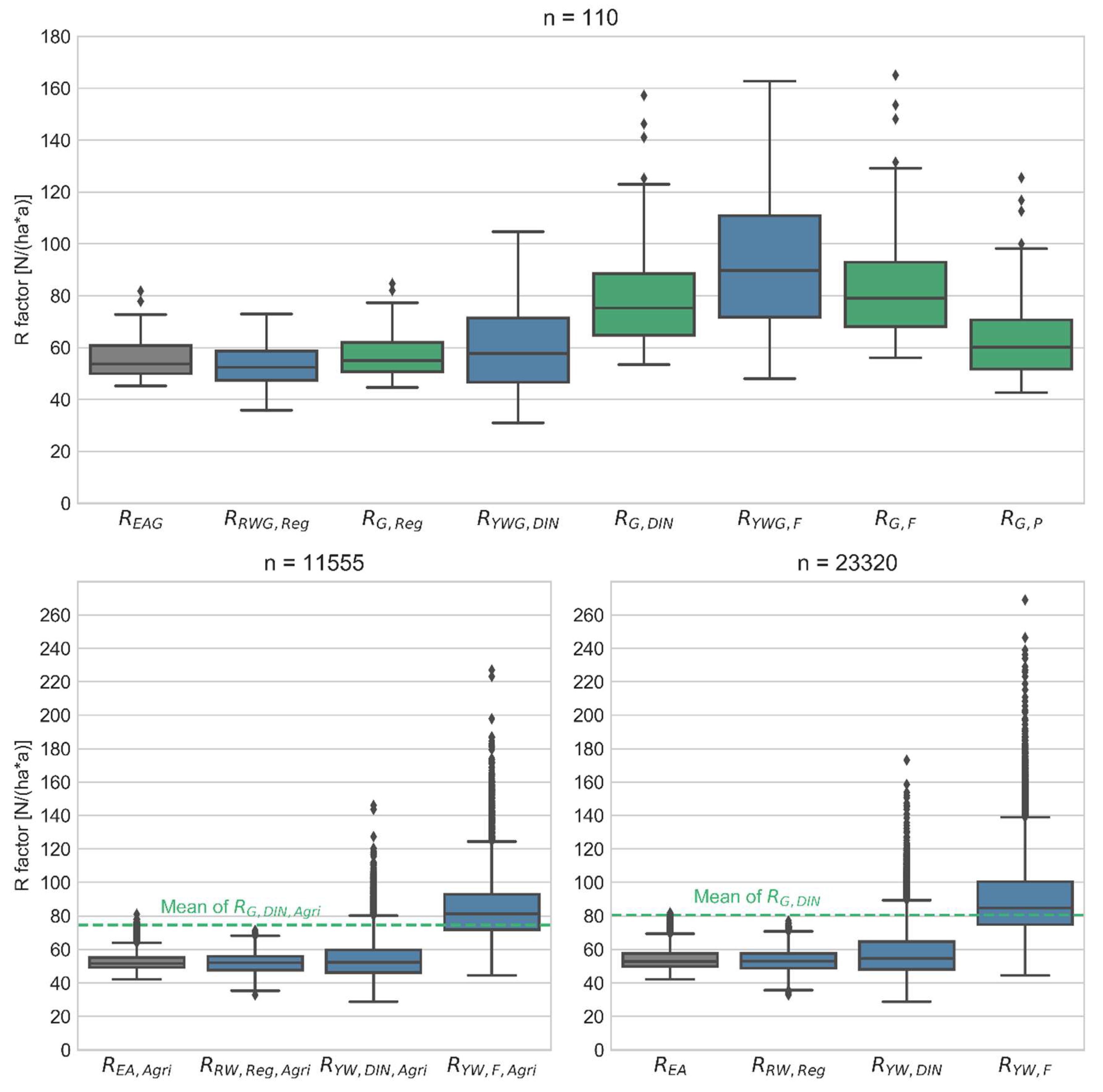
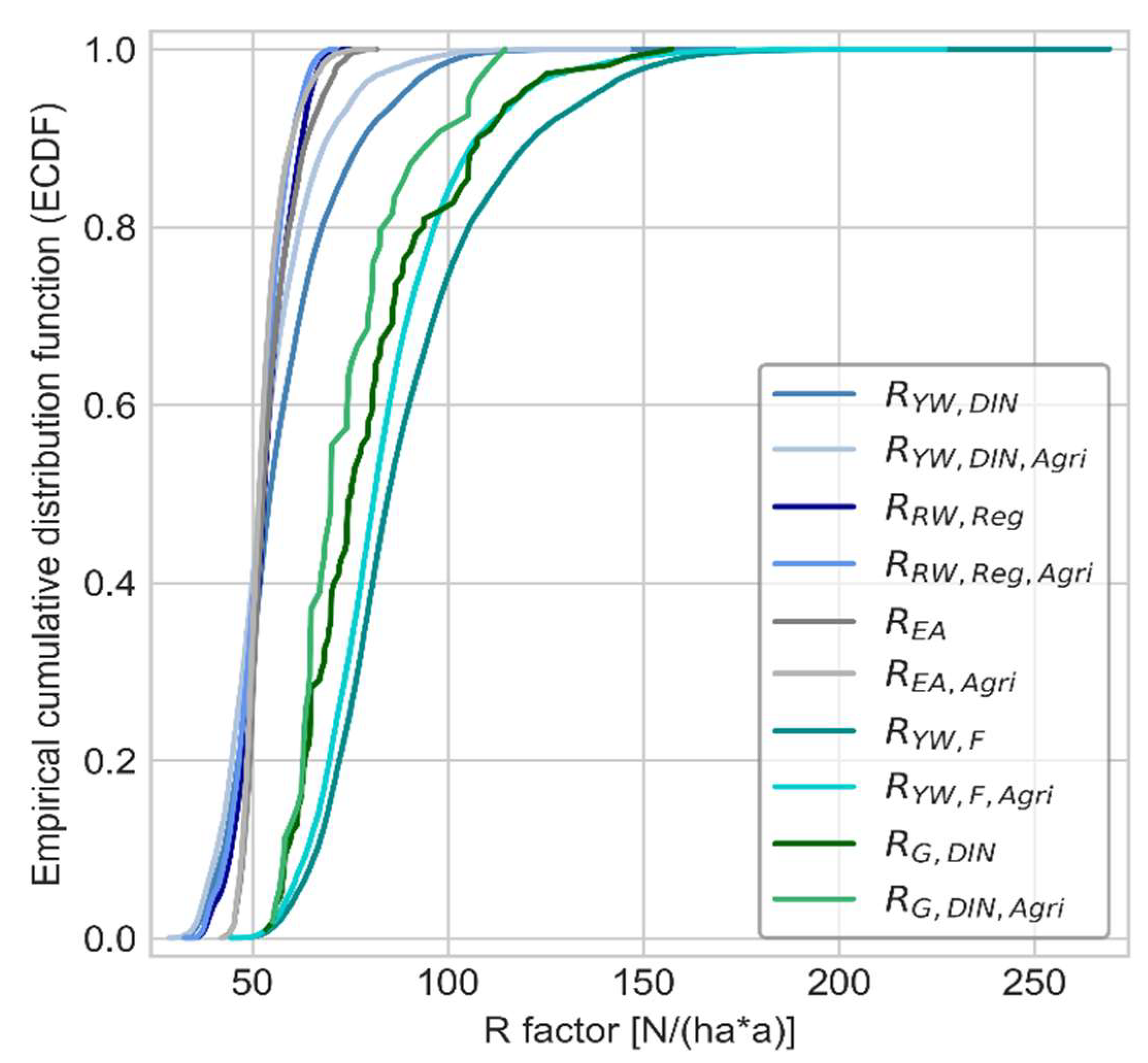
3.1. Statistical Comparison of the Calculated R-factors

The R-factor R_YW,DIN calculated from the original unscaled RADKLIM YW product according to DIN 19708 ranges between 28.8 and 173.2 kJ/m² mm/h with an average value of 58.0 kJ/m² mm/h (see

Table 2. Statistical summary of all R-factor derivatives.

R-factor	n	Method	Data Source	Mean	Standard Deviation	Min	Median	Max
RYW,DIN	23,320	DIN 19708	RADKLIM	58.0	14.7	28.8	54.6	173.2
RYW,DIN,Agri	11,555	DIN 19708	RADKLIM	54.2	12.0	28.8	52.3	146.1
RG,DIN	110	DIN 19708	Gauges	80.6	20.6	53.4	75.3	157.2
RYWG,DIN	110	DIN 19708	RADKLIM	60.1	15.8	31.0	57.8	104.7
REA	23,320	Regression	Erosion atlas	54.5	6.6	42.1	52.8	81.8
REA,Agri	11,555	Regression	Erosion atlas	52.8	5.3	42.1	51.7	81.0
RRW,Reg	23,320	Regression	RADKLIM	53.2	6.8	32.8	53.0	77.0
RRW,Reg,Agri	11,555	Regression	RADKLIM	51.9	6.4	32.8	52.1	71.4
RG,Reg	110	Regression	Gauges	57.0	8.8	44.7	55.0	84.7
RRWG,Reg	110	Regression	RADKLIM	53.1	7.8	35.9	52.4	73.0
REAG	110	Regression	Erosion atlas	55.9	8.1	45.2	53.7	81.8
RYW,F	23,320	DIN scaled	RADKLIM	90.1	22.8	44.5	84.8	269.1
RYW,F,Agri	11,555	DIN scaled	RADKLIM	84.2	18.6	44.5	81.3	227.0
RG,F	110	DIN scaled	Gauges	84.6	21.6	56.1	79.1	165.1
RYWG,F	110	DIN scaled	RADKLIM	93.4	24.6	48.0	89.8	162.7
RG,P	110	DIN scaled	Gauges	64.4	16.4	42.6	60.1	125.5

and Figure 2). It is thus 6.4% higher on average than the values of the erosion atlas R_EA, whereas its range is 263.7% higher and its standard deviation is 122.7% higher. R_YW,DIN shows thus a much higher variability than the strongly smoothed R_EA which was derived from spatially interpolated rainfall data using a regression equation (Equation (3)).

The R-factor calculated from the gauge dataset R_G,DIN has an average of 80.6 kJ/m² mm/h, which is 47.8% higher than the average value of R_EA and 39% higher than the average of R_YW,DIN. At 107 of 110 stations the rain gauges show higher R-factors than the corresponding pixels of the radar climatology. The average R-factor difference for all point-pixel pairs amounts to 20.5 kJ/m² mm/h between R_YWG,DIN and R_G,DIN. For the 72 stations operated by DWD, which were used for radar data adjustments, the average difference between R_YWG,DIN and R_G,DIN amounts to 19.1 kJ/m² mm/h, whereas the average difference at the 38 stations operated by HLNUG is slightly higher with 23.1 kJ/m² mm/h. Compared to the erosion atlas, all 110 rain gauge stations show higher R values with an average difference of 24.7 kJ/m² mm/h.

Using the regression equation from the erosion atlas (Equation (3)) and the RADKLIM RW product to derive R_RW,Reg yielded comparable values as R_EA with a slightly lower mean and maximum, significantly lower minimum, but a slightly higher median and standard deviation. For R_G,Reg, all statistical values were slightly higher than for R_EA and R_RW,Reg. Consequently, before scaling, the rain gauge dataset consistently produces the highest R-factors, but the magnitude of the differences is governed by the derivation method. The input dataset has little influence on the statistical characteristics of the outcome when using a regression equation and the major differences between these regression-based derivatives are the spatial resolutions and spatial distributions (see Section 3.2). When grouping all R-factor derivatives by the calculation method—irrespective of input data and spatial extent—the mean of those R-factors derived according to DIN 19708 (without scaling) is 9.1 kJ/m² mm/h higher than the mean of all R-factors derived using the regression equation. Furthermore, with 15.8 kJ/m² mm/h, the DIN method group showed on average a 122.2% higher standard deviation than the regression method group (7.1 kJ/m² mm/h), which underlines the smoothing effect that can be obtained by using a regression equation instead of the event-based method according to DIN 19708. The difference between both methods is particularly well illustrated by the very steep empirical cumulative distribution functions (ECDF) of all regression-based derivatives (see Figure 3).

Selecting pixels with cropland leads to an average decrease of R_YW,DIN by 3.8 kJ/m² mm/h (−6.6%). The minimum did not change, while the maximum decreased by 27.1 to 146.1 kJ/m² mm/h (see Figure 2 and Figure 3). Taking into account only the pixels with cropland and rain gauges, the count was reduced to 54 (a total of 54 rain gauges are located in radar pixels with cropland), the average R-factor (R_YWG,DIN,Agri) decreased also by 3.8 to 56.3 kJ/m² mm/h and the maximum decreased by 12.5 to 92.2 kJ/m² mm/h. For R_G,DIN, the impact of the data selection on the statistical distribution is considerably higher due to the smaller sample size. Its average decreased by 6.1 to 74.5 kJ/m² mm/h, whereby the maximum decreased by 42.5 to 114 kJ/m² mm/h when selecting only pixels with cropland. Consequently, the removal of many high erosivity values in the mountainous regions (see Figure A1), for which the uncertainty and underestimation of the radar data is particularly high, leads to a slightly better agreement of the R-factors calculated according to DIN 19708 from RADKLIM and rain gauge data. Grouping the nine R-factor derivatives based on R_YW,DIN, R_RW,Reg and R_EA by spatial extent resulted in a mean of 55.2 kJ/m² mm/h for all pixels of the study area, 52.9 kJ/m² mm/h for pixels with cropland and 56.3 kJ/m² mm/h for pixels with a rain gauge.

In regard to the data source, the results showing an underestimation of rainfall erosivity by the radar climatology compared to rain gauge data are in line with the outcomes of Fischer et al. (2018), thus the application of the proposed correction factors was considered to be useful and necessary. After scaling, the R-factors of the radar climatology and rain gauges correspond much better (see Figure 2 and Figure 3). The difference between the two datasets shifts in favour of the radar climatology, since on average R_YW,F is 8.8 kJ/m² mm/h higher than R_G,F (see Table 2). In comparison to R_EA, both R-factors were significantly higher after scaling. On average, R_YW,F was 65.3% higher and R_G,F was 58.5% higher than the R-factor R_EA of the erosion atlas. Although the correction factor proposed by Panagos et al. [23] reduces the R-factor to a level close to R_YW,DIN, R_G,P still showed an 18.2% higher mean than R_EA. Irrespective of the dataset used for derivation and the application of correction procedures, an increase of the R-factor compared to R_EA can thus be determined without doubt.

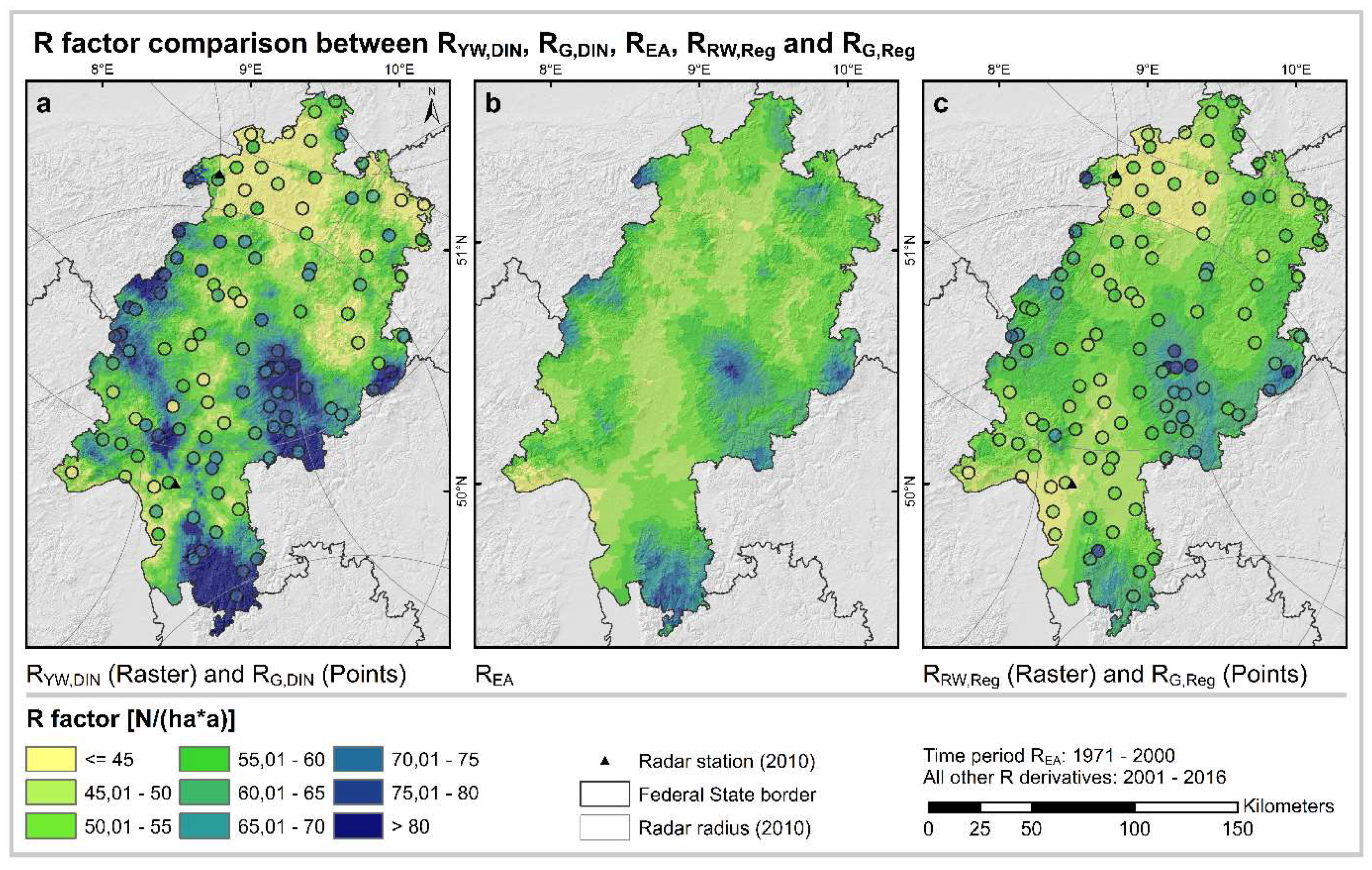
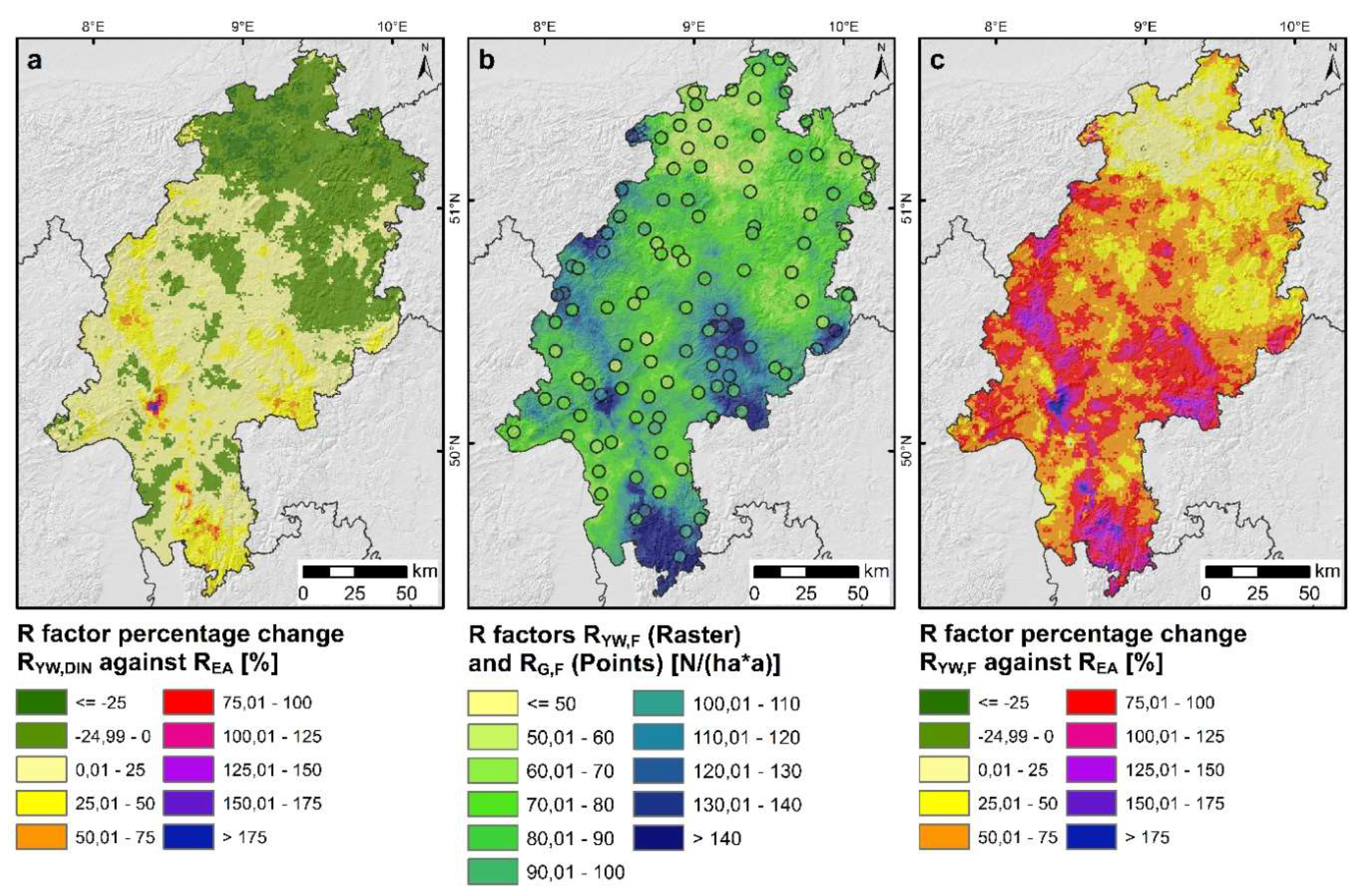
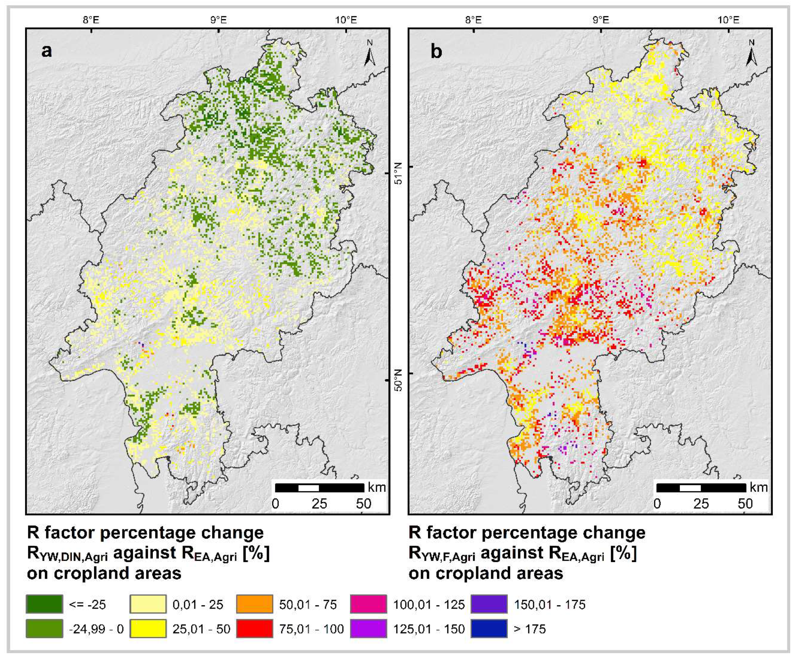
3.2. Spatial Distribution

For erosion control applications at a federal state scale which aim to identify regions with a particularly high risk of erosion, the spatial distribution of rainfall erosivity is actually more relevant than the absolute erosivity values. The lowest values of R_YW,DIN occur in the north of Hesse, around the West Hesse Depression, in an area for which no radar measurements were available during some months of the years 2007 and 2014 due to radar hardware upgrades. The average value of the annual R-factor without these two years shows that the minimum is nevertheless located in this area. This is therefore in accordance with the R-factor R_EA (calculation based on regression), which also shows a minimum in this area (see Figure 4). The areas of relatively low R-factors northwest of Fulda and in the Upper Rhine Plain correspond well in both datasets, too. In the north-east of Hesse, however, the newly calculated R-factor R_YW,DIN showed slightly lower erosivity over a large area with a similar spatial distribution. Both datasets showed an increase of the R-factor with increasing terrain height, whereby R_YW,DIN showed significantly higher values over a large area, especially in the Odenwald, Taunus, Westerwald and at Vogelsberg. However, at Vogelsberg, a weakness of the radar climatology to correctly quantify precipitation at higher altitudes was evident as the increase of the R-factor in the lower slope areas was considerably higher than in the summit area. In the area of Wetterau, a negative spoke of the Frankfurt Radar was clearly visible in R_YW,DIN and all other R-factors derived from RADKLIM. Still, in this area an increase of the R-factor compared to the erosion atlas can be seen in most of the grid cells, in some places even up to 45% (see Figure 5a).

The scaling is able to compensate for the underestimation of the R-factor by the radar climatology, which becomes particularly obvious in the northern parts of Hesse where the difference to the erosion atlas shows mostly positive values except for a few single pixels (see Figure 5c). Moreover, Figure 5b shows much better conformity with R_G,DIN in the entire study area, which has already been indicated in the previous section.

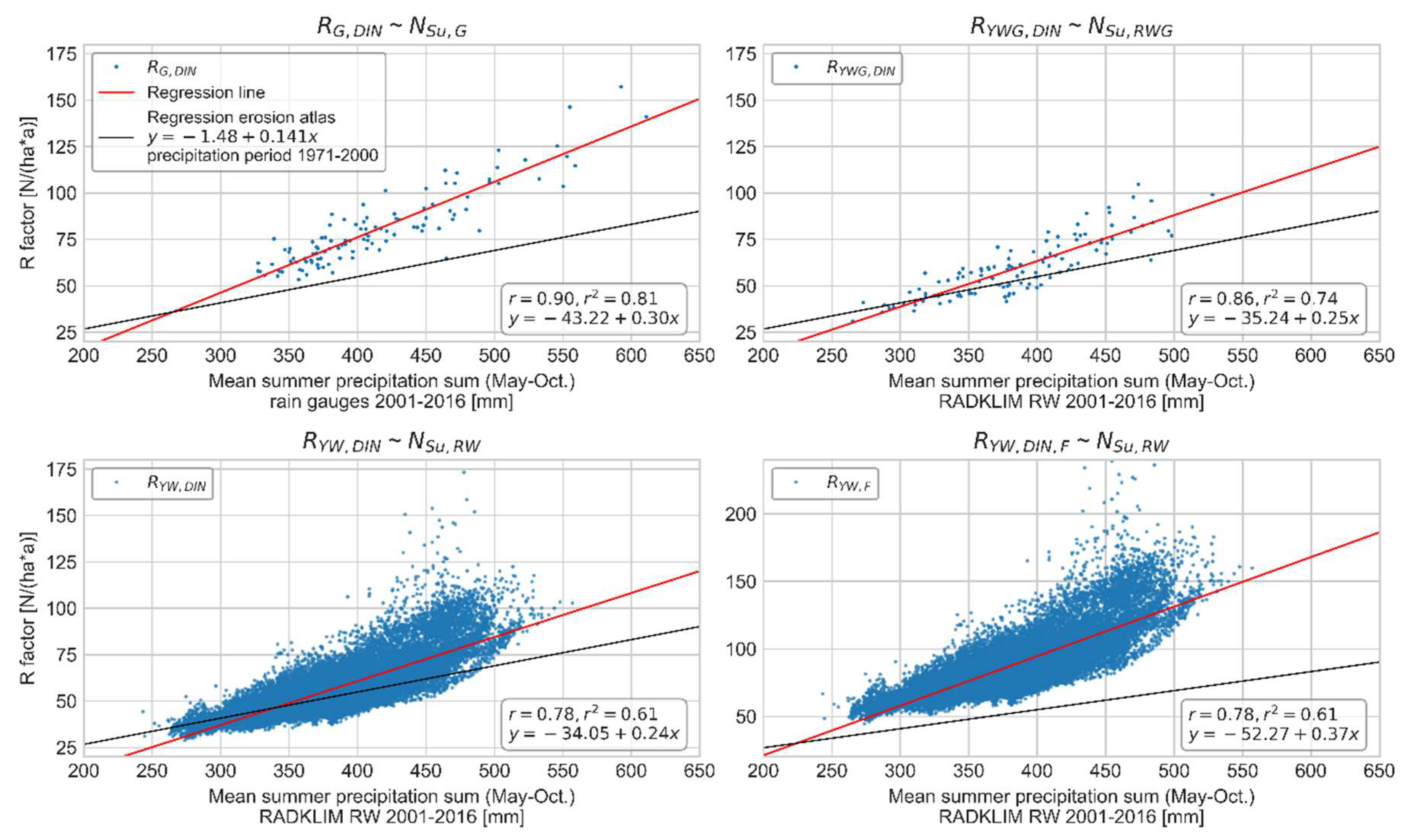
3.3. Derivation of Updated Regression Equations

The statistical comparisons in Section 3.1 show consistently lower values for all R-factors derived by means of regression. Besides the method itself and the input data source, the observation time period of the data used for the derivation of the regression equation might play a role due to climate change, which is why we derived an updated regression equation for comparison.

The new regression equations derived from the rain gauge data and the radar climatology both show a strong correlation between summer precipitation and R-factor. The fitted regression line has a considerably higher slope than the original one used for the erosion atlas (Equation (3)) (see Figure 6). Some data points of R_YW,DIN, which are mainly located in the area of the radar gap in northern Hesse, are still below the regression line from the erosion atlas. For R_G,DIN, however, all data points are above. Consequently, for the period 2001–2016, the regression equation used in the erosion atlas provides a value deviating from the R-factor according to DIN 19708 for all of the rain gauges.

When considering the newly derived regression equations from the radar climatology, it is striking that the equations for the entire data set and the pixels at the rain gauge locations are almost identical (see Figure 6). Consequently, the spatial distribution of the rain gauge locations can be regarded as very representative for mapping the overall distribution of rainfall erosivity in Hesse.

Another striking difference with regard to the sample size, however, is a series of several very high values of R_YW,DIN in the range between 400 and 500 mm summer precipitation. These are only included in the R-factor of the entire radar climatology dataset, but are not significantly reflected in the regression due to their relatively small number. Therefore, it can be assumed that extraordinarily intensive individual events have a strong impact due to the comparatively short time series. These events could only be detected by the high spatial resolution of the radar climatology and are not included in the rain gauge dataset.

Using the new regression equation derived from the rain gauges (R = −43.22 + 0.3 N_Su) with the summer precipitation sums of the RADKLIM RW product for the federal state of Hesse leads to a R-factor value range between 29.7 and 123.9 kJ/m² mm/h with an average of 73.2 kJ/m² mm/h. It has thus a significantly lower maximum than all event-based R-factor derivatives. Its mean value is slightly lower than that of R_G,DIN (80.6 kJ/m² mm/h) due to the slight overall underestimation of precipitation by the radar climatology, and lies approximately in the centre between the averages of R_YW,DIN (58 kJ/m² mm/h) and the corrected R_YW,F (90.1 kJ/m² mm/h).

4. Discussion

An evaluation of the radar climatology dataset revealed that it slightly underestimates precipitation quantities. This underestimation is particularly pronounced at higher altitudes and at high rainfall intensities [31]. In particular, the latter plays a decisive role for rainfall erosivity since rainfall intensity is directly linked to the kinetic energy of rainfall and, thus, its ability to detach soil particles. The assumption that the R-factor calculated from the radar climatology according to DIN 19708 without input data correction is too low could be confirmed by comparing it with the R-factor derived from the rain gauge dataset. However, irrespective of the dataset used for derivation, the spatial scale and the application of correction procedures, an increase of the R-factor compared to R_EA which is currently used in the technical information system erosion atlas Hesse [13] can be determined without doubt. This result highlights the need of updated R-factor methods for consultation and planning in Hesse.

The R-factors calculated by the regression equation from the erosion atlas, the summer precipitation sums of radar climatology, and rain gauges showed only slightly higher average values than the erosion atlas. Considering the significant differences to the R-factor derivations according to DIN 19708, this indicates that the regression equation used for the erosion atlas, which was derived from precipitation data of the 1960s, 70s and 80s, is no longer representative of the current climate conditions. Apparently, although there has only been a small increase in summer precipitation, there is a change in the heavy rainfall characteristics and/or in the relationship between erosive rainfall and total precipitation amount. This observation is in line with the projected changes in precipitation characteristics with regard to climate change. For most of Europe, it is expected that precipitation will increase during winter and decrease during summer [32,33]. Furthermore, the number of wet days is expected to decrease, whereas the intensity and the return levels of daily precipitation events will increase [12,32,34,35]. The combination of increasingly intense heavy rainfall and the reduced water infiltration capacity of dry soils is expected to amplify the risk of floods [36] and is also very likely to increase soil erosion. These observations indicate that the validity of regression equations for R-factor calculation might decrease, particularly if mean summer precipitation sums are used instead of mean annual sums. An additional influencing factor for higher R-factors calculated from rain gauge data could be the better recording of intensity peaks by more accurate modern rain gauges as opposed to the less accurate rain gauges used to collect the data for the 1971–2000 dataset [37].

Despite the discussed limitations, the regression-based approach has the advantage that it is much easier to apply in practice than the method according to DIN 19708, which is computationally much more expensive, especially when using it on spatially highly resolved data such as the radar climatology. Moreover, the use of a regression equation with precipitation sums always leads to a certain smoothing and is thus more robust against outliers than the event-based method when only comparatively short precipitation time series are available. However, as our results have clearly shown, the regression approach also requires frequent updates of the equations and hence a certain maintenance of the methodology. Obviously, updates to the equations rely on the availability of rain gauge data. For Germany, this is not a major issue anymore since temporally highly resolved rain gauge data are freely available at the DWD Open Data Portal. In other countries, however, this may be a greater obstacle.

With regard to the scaling of the R-factors which was proposed in recent studies [22,23], it should be noted that a correction that increases the RADKLIM R-factor is undoubtedly necessary to compensate for the systematic underestimation of precipitation data obtained from radar climatology. However, the degree of correction is difficult to estimate due to a lack of reference. If the scaled R-factor of the rain gauge dataset R_G,F is regarded as a correct reference for validation, the correction applied for R_YW,F and R_YWG,F appears somewhat too high, especially when looking at Figure 2. When considering the identical sample size and the largely consistent location of the point-pixel data pairs of R_YWG,F, the advantage of the radar and the fact that more events tend to be recorded hardly matters. However, the median of R_YWG,F almost corresponds to the third quartile of R_G,F. Here, a direct transferability of the correction factors, which were derived from a four-year series of measurements of 12 rain gauges within one square kilometre in Bavaria [22], may be limited. Further research efforts and measurements to extend these time series and derive correction factors of higher spatial representativity from more than one single raster cell would have the potential to significantly reduce the uncertainty when using radar climatology data—not only for rainfall erosivity estimation but for applications related to heavy rainfall in general.

In contrast, the scaling according to Panagos et al. [23] to compensate for the temporal resolution of the input data provides very questionable results. Taking into account the conducted plausibility check of the radar climatology and the comparisons with the rain gauge data by Kreklow et al. [31], an underestimation of the R-factor by the radar data is clearly demonstrated. Since the correction factor proposed by Panagos et al. [23] reduces the R-factor of the rain gauges to a level almost identical to that of the radar climatology, a correction factor that is too low must be assumed. The correction factor does not appear to be representative for Hesse, due to the fact that its derivation is based on a rain gauge dataset for the whole of Europe and equally includes data from maritime, continental, temperate, subpolar and Mediterranean climates. Already for the two neighbouring countries Austria and Italy, Fiener et al. [38] found significant differences in the magnitude and monthly distribution of the R-factor, which indicates a lack of spatial representativity of the temporal scaling factor proposed by Panagos et al. [23]. Such representativity issues have been subject to discussion between the authors [4,38,39]. In addition, the original methodology for the calculation of the R-factor is based on continuous precipitation recordings, which were aggregated to intervals of constant intensity [1]. Consequently, a temporal resolution of 1 min as a lowest reference chosen by Fischer et al. [22] is much closer to the original method than the reference resolution of 30 min used by Panagos et al. [23]. The much lower reference resolution used by Panagos et al. [23] thus explains the significantly lower temporal correction factor compared to the factor proposed by Fischer et al. [22].

With regard to practical application, it is recommended that the R-factor map currently used in the erosion atlas should be updated. Our results show that the first and most important step is to use more recent precipitation data for derivation, which are more representative under current climate conditions. Obviously, using the event-based method according to DIN 19708 with radar climatology, which was proposed by Auerswald et al. [6], provides the R-factor with the highest spatial detail, but it may be locally biased by some extreme rainfall events or radar artefacts which are not balanced out in the comparatively short radar time series. Moreover, a correction of R-factors derived from radar climatology according to DIN 19708 is necessary to compensate for underestimation, but the level of correction required is still subject to discussion. However, the radar climatology time series is still considerably longer than the time series used for deriving the original regression equations by Sauerborn [9], of which one was also used in the erosion atlas Hesse. Consequently, during a transition period, the most robust and easy-to-use approach to obtain updated R-factors is by using an updated regression equation derived from recent rain gauge data with summer precipitation sums calculated from radar climatology data. On the one hand, this approach accounts for climate change by increasing the R-factors according to reliable rain gauge observations. On the other hand, it makes use of the high spatial resolution of radar data and comprises a certain smoothing, since precipitation sums are less biased by local extreme events and by the underestimation of high rainfall intensities by weather radar in comparison to the event-based R-factors derived according to DIN 19708. Moreover, due to less snowfall and thus fewer uncertainties in the radar climatology data during the summer half-year, the use of radar-based summer precipitation sums increases the robustness of the recommended method compared to the use of radar-based annual precipitation sums.

Due to the central location of Hesse within Germany, the recommended updated regression equation based on rain gauge data for Hesse (R = −43.22 + 0.3 N_Su) has a high transferability for most of Germany. However, for federal states in northern and eastern Germany which have a more maritime or continental climate, regional regression equations should be calculated from recent local rain gauge data.

5. Conclusions

In this study, we compared several derivation approaches for the R-factor of the USLE and evaluated the performance of radar climatology and rain gauge data for different methods and three spatial extents. Moreover, two correction factors proposed in other studies were tested and updated regression equations were derived for the German federal state of Hesse.

Regarding the three hypotheses put forward at the beginning of this study, our results can be summarised as follows:

1. The newly derived R-factors from rain gauge and radar climatology data are indeed higher than the R-factors from existing calculations due to climate and weather changes. For the study period of 2001–2016, the regression equation used in the erosion atlas provides a lower R-factor than DIN 19708 for all of the rain gauges.

2. The contradiction between the theoretically higher R-factor of the radar climatology due to the more complete recording of all erosive rainfall events on the one hand and the underestimation of the R-factor due to the attenuation of intensity peaks, on the other hand, could be established. In the spatial average as well as when looking at the point-pixel data pairs, which largely eliminates the influence of the higher spatial resolution of the radar climatology data, the R-factors of the rain gauges are significantly higher. However, when looking at the entire radar data set, some strikingly high R-factor values, which were not captured by the rain gauges, become apparent. Due to their comparatively small number, however, they have no significant influence on the spatial mean value. In addition, these extraordinary high R-factors can also be a result of very intensive rainfall events in the comparatively short observation period that might be smoothed by prolonging the radar climatology dataset. The correction of the R-factors according to Fischer et al. [22] provides an improvement of the results for the radar climatology, although a possible overcorrection cannot be excluded.

3. The spatial distribution of the newly calculated R-factor according to DIN 19708 and that from the erosion atlas show a relatively good conformity with minima and maxima in similar regions as well as a consistent mapping of a relief dependency. In the northeast of Hesse, the R-factor calculated from the uncorrected radar climatology according to DIN 19708 shows comparatively lower values than the erosion atlas. In contrast, it also shows large areas of higher R-factor values than the erosion atlas, especially in the ridges of the low mountain ranges and in the central lowland areas of Hesse, for example, the Wetterau. The updated regression equations, which are almost identical for all radar pixels and the point-pixel data pairs, indicate that the rain gauge locations are very representative for mapping the overall spatial distribution of rainfall erosivity in the study area.

The results of this study clearly indicate that the R-factor map currently used in the erosion atlas should be updated. For a transition period until the radar climatology time series is long enough to compensate for bias from extraordinarily intensive rainfall events, it is recommended to apply a new regression equation derived from recent rain gauge measurements with summer precipitation sums calculated from radar climatology data.

With the progressive improvement of the data basis (time series, quality and correction), however, radar climatology data will be further incorporated into operational applications such as risk management and erosion consulting.

References

1. Wischmeier, W.H.; Smith, D.D. Predicting Rainfall Erosion Losses. A Guide to Conservation Planning; Agriculture handbook number 537; U.S. Department of Agriculture: Washington, DC, USA, 1978.
2. Schwertmann, U.; Vogl, W.; Kainz, M. Bodenerosion durch Wasser. Vorhersage des Abtrags und Bewertung von Gegenmaßnahmen, 2. Aufl.; Ulmer: Stuttgart, Germany, 1990; ISBN 3800130882. [Google Scholar]
3. Deutsches Institut für Normung. DIN 19708. Bodenbeschaffenheit—Ermittlung der Erosionsgefährdung von Böden durch Wasser mithilfe der ABAG; Normenausschuss Wasserwesen im DIN: Berlin, Germany, 2005; (19708). [Google Scholar]
4. Panagos, P.; Ballabio, C.; Borrelli, P.; Meusburger, K.; Klik, A.; Rousseva, S.; Tadic, M.P.; Michaelides, S.; Hrabalikova, M.; Olsen, P.; et al. Rainfall erosivity in Europe. Sci. Total Environ. 2015, 511, 801–814. [Google Scholar] [CrossRef] [PubMed] [Green Version]
5. Fischer, F.; Hauck, J.; Brandhuber, R.; Weigl, E.; Maier, H.; Auerswald, K. Spatio-temporal variability of erosivity estimated from highly resolved and adjusted radar rain data (RADOLAN). Agric. For. Meteorol. 2016, 223, 72–80. [Google Scholar] [CrossRef]
6. Auerswald, K.; Fischer, F.K.; Winterrath, T.; Brandhuber, R. Rain erosivity map for Germany derived from contiguous radar rain data. Hydrol. Earth Syst. Sci. 2019, 23, 1819–1832. [Google Scholar] [CrossRef] [Green Version]
7. Tetzlaff, B.; Friedrich, K.; Vorderbrügge, T.; Vereecken, H.; Wendland, F. Distributed modelling of mean annual soil erosion and sediment delivery rates to surface waters. CATENA 2013, 13–20. [Google Scholar] [CrossRef]
8. Deutsches Institut für Normung. DIN 19708. Bodenbeschaffenheit—Ermittlung der Erosionsgefährdung von Böden durch Wasser mit Hilfe der ABAG, 2017–08; Beuth Verlag GmbH: Berlin, Germany, 2017. [Google Scholar]
9. Sauerborn, P. Die Erosivität der Niederschläge in Deutschland. Ein Beitrag zur quantitativen Prognose der Bodenerosion durch Wasser in Mitteleuropa. Ph.D. Thesis, Inst. für Bodenkunde, Bonn, Germany, 1994. [Google Scholar]
10. Elhaus, D. Erosionsgefährdung. Informationen zu den Auswertungen der Erosionsgefährdung durch Wasser, Germany. 2015. Available online: https://www.gd.nrw.de/zip/erosionsgefaehrdung.pdf (accessed on 11 March 2020).
11. Burt, T.; Boardman, J.; Foster, I.; Howden, N. More rain, less soil: Long-term changes in rainfall intensity with climate change. Earth Surface Process. Landf. 2016, 41, 563–566. [Google Scholar] [CrossRef] [Green Version]
12. Fiener, P.; Neuhaus, P.; Botschek, J. Long-term trends in rainfall erosivity–analysis of high resolution precipitation time series (1937–2007) from Western Germany. Agric. For. Meteorol. 2013, 171-172, 115–123. [Google Scholar] [CrossRef]
13. Friedrich, K.; Schmanke, M.; Tetzlaff, B.; Vorderbrügge, T. Erosionsatlas Hessen. In Proceedings of the Tagungsband d. Jahrestagung der DBG/BGS, Kommission VI, “Erd-Reich und Boden-Landschaft“, Bern, Switzerland, 24–27 August 2019. DBG/BGS, Ed.. [Google Scholar]
14. Hessisches Landesamt für Naturschutz, Umwelt und Geologie (HLNUG). BodenViewer Hessen. Available online: http://bodenviewer.hessen.de/mapapps/resources/apps/bodenviewer/index.html?lang=de (accessed on 21 January 2020).
15. Rogler, H.; Schwertmann, U. Erosivität der Niederschläge und Isoerodentkarte Bayerns. Z. für Kult. und Flurberein. 1981, 22, 99–112. [Google Scholar]
16. Hessisches Landesamt für Naturschutz, Umwelt und Geologie (HLNUG). R-Faktor. Available online: https://www.hlnug.de/themen/boden/auswertung/bodenerosionsbewertung/bodenerosionsatlas/r-faktor (accessed on 16 January 2020).
17. Donat, M.G.; Alexander, L.V.; Yang, H.; Durre, I.; Vose, R.; Dunn, R.J.H.; Willett, K.M.; Aguilar, E.; Brunet, M.; Caesar, J.; et al. Updated analyses of temperature and precipitation extreme indices since the beginning of the twentieth century: The HadEX2 dataset. J. Geophys. Res. Atmos. 2013, 118, 2098–2118. [Google Scholar] [CrossRef]
18. Winterrath, T.; Brendel, C.; Hafer, M.; Junghänel, T.; Klameth, A.; Lengfeld, K.; Walawender, E.; Weigl, E.; Becker, A. Radar climatology (RADKLIM) version 2017.002 (YW); gridded precipitation data for Germany. Available online: https://search.datacite.org/works/10.5676/dwd/radklim_yw_v2017.002 (accessed on 25 June 2019).
19. Winterrath, T.; Brendel, C.; Hafer, M.; Junghänel, T.; Klameth, A.; Walawender, E.; Weigl, E.; Becker, A. Erstellung einer radargestützten Niederschlagsklimatologie; Berichte des Deutschen Wetterdienstes No. 251; 2017; Available online: https://www.dwd.de/DE/leistungen/pbfb_verlag_berichte/pdf_einzelbaende/251_pdf.pdf?__blob=publicationFile&v=2 (accessed on 29 March 2019).
20. Kreklow, J.; Tetzlaff, B.; Burkhard, B.; Kuhnt, G. Radar-Based Precipitation Climatology in Germany—Developments, Uncertainties and Potentials. Atmosphere 2020, 11. [Google Scholar] [CrossRef] [Green Version]
21. Bronstert, A.; Agarwal, A.; Boessenkool, B.; Crisologo, I.; Fischer, M.; Heistermann, M.; Köhn-Reich, L.; López-Tarazón, J.A.; Moran, T.; Ozturk, U.; et al. Forensic hydro-meteorological analysis of an extreme flash flood: The 2016-05-29 event in Braunsbach, SW Germany. Sci. Total Environ. 2018, 977–991. [Google Scholar] [CrossRef]
22. Fischer, F.K.; Winterrath, T.; Auerswald, K. Temporal- and spatial-scale and positional effects on rain erosivity derived from point-scale and contiguous rain data. Hydrol. Earth Syst. Sci. 2018, 22, 6505–6518. [Google Scholar] [CrossRef] [Green Version]
23. Panagos, P.; Borrelli, P.; Spinoni, J.; Ballabio, C.; Meusburger, K.; Beguería, S.; Klik, A.; Michaelides, S.; Petan, S.; Hrabalíková, M.; et al. Monthly Rainfall Erosivity: Conversion Factors for Different Time Resolutions and Regional Assessments. Water 2016, 8, 119. [Google Scholar] [CrossRef] [Green Version]
24. Semmel, A. Hessisches Bergland. In Physische Geographie Deutschlands, 2nd ed.; Liedtke, H., Marcinek, J., Eds.; Justus Perthes Verlag: Gotha, Germany, 1995; pp. 340–352. ISBN 3-623-00840-0. [Google Scholar]
25. Winterrath, T.; Brendel, C.; Hafer, M.; Junghänel, T.; Klameth, A.; Lengfeld, K.; Walawender, E.; Weigl, E.; Becker, A. Radar climatology (RADKLIM) version 2017.002 (RW); gridded precipitation data for Germany. Available online: https://search.datacite.org/works/10.5676/dwd/radklim_rw_v2017.002 (accessed on 25 June 2019).
26. Deutscher Wetterdienst Open Data Portal. Rain Gauge Precipitation Observations in 1-Minute Resolution. Available online: https://opendata.dwd.de/climate_environment/CDC/observations_germany/climate/1_minute/precipitation/ (accessed on 20 February 2020).
27. Kreklow, J.; Tetzlaff, B.; Kuhnt, G.; Burkhard, B. A Rainfall Data Intercomparison Dataset of RADKLIM, RADOLAN, and Rain Gauge Data for Germany. Data 2019, 4. [Google Scholar] [CrossRef] [Green Version]
28. The HDF Group. Hierarchical Data Format. Available online: https://portal.hdfgroup.org (accessed on 18 December 2018).
29. Mckinney, W. pandas: A Foundational Python Library for Data Analysis and Statistics. Python High-Perform. Sci. Comput. 2011, 14. [Google Scholar]
30. Kreklow, J. Facilitating radar precipitation data processing, assessment and analysis: A GIS-compatible python approach. J. Hydroinformatics 2019, 21, 652–670. [Google Scholar] [CrossRef] [Green Version]
31. Kreklow, J.; Tetzlaff, B.; Burkhard, B.; Kuhnt, G. Radar-Based Precipitation Climatology in Germany - Developments, Uncertainties and Potentials. Available online: https://www.preprints.org/manuscript/202002.0044/v1 (accessed on 10 February 2020).
32. Field, C.B.; Barros, V.R.; Dokken, D.J.; Mach, K.J.; Mastrandrea, M.D. Climate Change 2014 – Impacts, Adaptation and Vulnerability: Part A: Global and Sectoral Aspects; Working Group II Contribution to the IPCC Fifth Assessment Report; IPCC: Geneva, Switzerland, 2015; Available online: https://www.cambridge.org/core/books/climate-change-2014-impacts-adaptation-and-vulnerability-part-a-global-and-sectoral-aspects/1BE4ED76F97CF3A75C64487E6274783A (accessed on 7 February 2018).
33. Giorgi, F.; Bi, X.; Pal, J. Mean, interannual variability and trends in a regional climate change experiment over Europe. II: climate change scenarios (2071–2100). Clim. Dyn. 2004, 23, 839–858. [Google Scholar] [CrossRef]
34. Semmler, T.; Jacob, D. Modeling extreme precipitation events—A climate change simulation for Europe. Glob. Planet. Chang. 2004, 44, 119–127. [Google Scholar] [CrossRef]
35. Frei, C.; Schöll, R.; Fukutome, S.; Schmidli, J.; Vidale, P.L. Future change of precipitation extremes in Europe: Intercomparison of scenarios from regional climate models. J. Geophys. Res. 2006, 111, 224. [Google Scholar] [CrossRef] [Green Version]
36. Kyselý, J.; Beranová, R. Climate-change effects on extreme precipitation in central Europe: Uncertainties of scenarios based on regional climate models. Theor. Appl. Clim. 2009, 95, 361–374. [Google Scholar] [CrossRef]
37. Quirmbach, M.; Einfalt, T.; Langstädtler, G.; Janßen, C.; Reinhardt, C.; Mehlig, B. Extremwertstatistische Untersuchung von Starkniederschlägen in NRW (ExUS). Korresp. Abwasser und Abfall 2013, 60, 591–599. [Google Scholar]
38. Fiener, P.; Auerswald, K. Comment on “The new assessment of soil loss by water erosion in Europe” by Panagos et al. (Environmental Science & Policy 54 (2015) 438–447). Environ. Sci. Policy 2016, 57, 140–142. [Google Scholar] [CrossRef]
39. Panagos, P.; Meusburger, K.; Ballabio, C.; Borrelli, P.; Beguería, S.; Klik, A.; Rymszewicz, A.; Michaelides, S.; Olsen, P.; Tadić, M.P.; et al. Reply to the comment on "Rainfall erosivity in Europe" by Auerswald et al. Sci. Total Environ. 2015, 532, 853–857. [Google Scholar] [CrossRef] [PubMed] [Green Version]
Figure 1. (a) Location, height above sea level [m] and selected landscape units of the federal state of Hesse, (b) spatial distribution of cropland areas in the study area.
Water 12 01424 g001
Figure 2. Boxplots of all R-factor derivatives grouped by spatial extent. In the lower subplots, the average of the rain gauges (RG,DIN) and the rain gauges in pixels with cropland (RG,DIN,Agri) have been added as a ground-truth reference. See Table 1 for explanation of the used abbreviations.
Water 12 01424 g002
Figure 3. Empirical cumulative distribution functions (ECDF) for all spatially highly resolved R-factor derivatives. The ECDFs for the rain gauges (RG,DIN) and the rain gauges in pixels with cropland (RG,DIN,Agri) have been added as a ground-truth reference.
Water 12 01424 g003
Figure 4. R-factor comparison between RYW,DIN, RG,DIN (a), REA (b), RRW,Reg and RG,Reg (c).
Water 12 01424 g004
Figure 5. R-factor percentage change of RYW,DIN against REA (a), scaled R-factors RYW,F and RG,F (b) and percentage change of RYW,F against REA (c).
Water 12 01424 g005
Figure 6. Comparison of regression models between different R-factors and the respective mean summer precipitation sums.
Water 12 01424 g006