Abstract
To assist waste management decision-making, there is a need to assess the economics of commercial-scale reuse of recirculating aquaculture system (RAS) effluent in horticulture. This study compared the feasibility/viability of using two representative horticulture systems, considering their distinct hydrological characteristics, in horticultural reuse schemes for RAS effluent. These representative systems included a soil-based system in field conditions (SOIL-FIELD) and a hydroponic system in greenhouse conditions (HYDRO-GH). A novel two-step hydro-economic modelling approach was used to quantify and compare the effluent storage volume, total land area, capital expenditure and crop price required for feasible/viable end-of-pipe reuse in the two systems. The modelling assessed several water management scenarios across four Australian climates. Results showed HYDRO-GH, reusing 100% of the annual effluent load and targeting an internal rate of return of 11.0%, required approximately 3 times more land, 14 times more capital expenditure and 5 times the crop price of SOIL-FIELD, targeting a 3.6% internal rate of return. As well as comparing two horticulture systems, this study presents a method to assess feasibility/viability of horticultural reuse schemes for other industrial wastewaters, using a water balance design approach.
1. Introduction
To meet the growing demand for aquaculture products amidst increasing resource scarcity [1,2], many aquaculture systems will need to produce more fish with less natural resources, while simultaneously minimizing their environmental impact. This is a process referred to as ‘sustainable intensification’ [3]. Sustainable intensification in aquaculture can be achieved by adapting existing production systems, or by adopting more efficient production systems [4].
Recirculating aquaculture systems (RASs) are a form of intensive, land-based fish production system, where water is recirculated between tanks and treatment components to enable water reuse and high fish stocking densities. Containment and water reuse in a RAS enables greater control over production, tighter biosecurity, and the potential to achieve high water- and land-use efficiency compared to other aquaculture systems [4,5,6,7,8]. As a result of intensification, freshwater RASs produce a concentrated effluent stream containing dissolved and solid waste fractions, including high concentrations of nitrogen, phosphorus, and plant-growth-promoting microorganisms well suited to reuse in horticulture [9,10]. In recent decades, RAS use has increased in industrialized nations. This trend looks set to continue as production of high-value farmed fish increases, and as production is forced into contained systems, due to limited availability of licenses in natural water bodies and restrictions on open or flow-through systems [1,11,12,13,14,15]. Predicted growth in RAS use makes utilization of the waste stream a critical priority in improving economic viability and sustainability of RAS [8].
Despite the compatibility of RAS effluent with horticulture, conventional management of the effluent stream often involves ‘end-of-pipe’ primary and secondary treatment. Treatment aims to reduce solids and nutrient concentrations prior to disposal, using land application, evaporation ponds, sewer or environmental discharge [16]. For RAS operators and resource managers, conventional effluent management may be considered a low-risk, low-maintenance solution compared to horticultural reuse. Treatment and disposal of effluent, however, represents capital and operational costs to RAS operators. Furthermore, where reuse is feasible, treatment and disposal represents a missed opportunity to generate additional income and further increase resource use efficiency in line with the waste hierarchy [17,18,19], considering the waste reductions already achieved within the RAS. Reuse, however, would need to be practically feasible and economically viable to encourage a shift from conventional treatment and disposal. To assist waste management decision-making, it is therefore important to clearly understand the feasibility/viability of end-of-pipe horticultural reuse schemes (HRSs) for RAS [8]. Fortunately, many studies have already demonstrated the plant-scale feasibility of reusing RAS effluent as irrigation in horticulture systems.
A relatively recent body of research into decoupled aquaponic systems has demonstrated the potential for end-of-pipe reuse of RAS effluent in hydroponic systems [20,21,22,23]. Decoupled aquaponic research has demonstrated that end-of-pipe hydroponic systems can generate yields equivalent to those achieved in commercial hydroponic systems, by supplementing deficient nutrients using inorganic fertilizers [24,25]. End-of-pipe hydroponic systems can also improve plant growth when using RAS effluent by adding aerobically and anaerobically mineralized sludge, the second waste stream from RAS [26,27]. Unlike coupled aquaponics, these improvements to plant production are all proven to be possible without impacting fish production [20]. Much of the recent research into decoupled aquaponics has focused on reuse in high-tech greenhouses [21,23,25,28], employing artificial lighting and temperature control to achieve high yields and high water- and land-use efficiency, although at the expense of high capital and operational costs [29,30]. Due to the high capital and operational costs, it may be unlikely that such high-tech systems, represented by (e) in Figure 1, would be feasible or viable for a commercial-scale RAS interested in horticultural reuse. Similarly, for ‘high-tech horticulturalists’ to locate their facility within pumping distance of a RAS, water resources might have to be the critically limiting factor for horticulture [30], which may be unlikely in many scenarios.
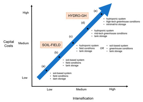
Figure 1.
Conceptual intensification spectrum, with capital costs for end-of-pipe horticultural reuse schemes (HRSs), including the two systems modelled in this study.
A separate body of research has focused on reuse of RAS effluent in low-tech soil-based systems in field conditions. These systems could be represented by (a) and (b) in Figure 1. Plant-scale findings have shown that plant production in soil-based systems responds well to high nutrient concentrations in effluent from intensive systems such as RAS [31], compared to that from less intensive aquaculture systems [32,33,34,35]. From an economic perspective, soil-based systems are lower cost compared to hydroponic systems, but generate lower yields [36] and typically lower financial returns [37,38]. Despite lower returns, in a commercial-scale HRS, soil-based systems in field conditions may offer several advantages over hydroponic-greenhouse systems. Soil-based systems in an HRS may have a lower land requirement due to greater water use per unit area [39,40], and can also directly receive RAS sludge without requiring treatment to mineralize nutrients [18], as required for typical hydroponic systems.
By using results from the soil-based and decoupled aquaponic studies, it is possible to compare plant-scale performance between soil-based systems in field conditions and hydroponic systems in greenhouse conditions. However, for any existing or planned RAS considering commercial-scale effluent reuse in an HRS, such a comparison does not consider critical requirements for the scheme to be feasible/viable. Critical requirements for commercial-scale feasibility/viability include, but are not limited to:
- (1)
- access to the total land requirement to accommodate the size of the scheme, including the growing area and effluent storage area (i.e., practical feasibility)
- (2)
- capital expenditure required to fund the scheme
- (3)
- crop price to achieve the required profitability of the scheme [41] (i.e., economic viability).
These three critical requirements are expected to vary with horticulture system and, due to each horticulture system’s different hydrologic characteristics, be further impacted by climate [21] and water management practices, as described in 2.0 Theoretical Background. Other studies assessing the economics of HRS for RAS effluent have focused on a single horticulture system, with fixed water management practices in one climate [17,42]. No studies compare horticulture systems from other points on the intensification spectrum (Figure 1), or the impact of water management practices and/or climate.
This study aims to answer the research question, “how do the critical requirements for feasible/viable HRS for RAS effluent vary for horticulture systems, climate and water management scenarios?”. The study uses hydro-economic modelling to quantify and compare two representative horticulture systems: a soil-based system in field conditions (SOIL-FIELD), and a hydroponic system in greenhouse conditions (HYDRO-GH), represented as (b) and (d) respectively in Figure 1. The critical requirements are assessed across different climate and water management scenarios. Through the comparison, the study also develops a novel method to assess feasibility/viability of HRS for various forms of agricultural and industrial wastewaters.
2. Theoretical Background
As background to the modelling used in this study, the major conceptual design considerations for an end-of-pipe HRS for RAS effluent need to be discussed. These are (1) the horticulture component, including the horticulture system and growing environment, (2) the effluent storage component, and (3) water infrastructure to supply supplementary irrigation water and enable effluent disposal. The horticulture and effluent storage components should be sized to achieve a target water reuse rate, e.g., 100%, 50% or 25% reuse of the annual effluent load. Sizing for a target water reuse rate requires the use of a water balance design approach, rather than a nutrient balance approach. If nitrogen, phosphorus or other nutrient concentrations are below plant requirements, nutrient supplementation can occur at a relatively low cost. If nutrients exceed plant requirements, dilution can be practiced and factored into the water balance, as in Awad et al. [43], which focused on diluting salinity of treated municipal wastewater for irrigation, and as in Delaide et al. [24] and Delaide et al. [25], in which dilution followed by supplementation of deficient nutrients in RAS effluent was carried out. While there are these and other important nutrient related factors, such as nutrient transformation in storage and delivery to plants, the scope of this paper extends only to the hydrology of HRS.
Different hydrologic characteristics in horticultural components are expected to have a significant impact on the size and cost of the HRS, which further supports the use of a water balance design approach. Soil-based systems are exposed to additional water loss pathways through soil surface evaporation and deep percolation, as well as leaching fractions commonly used to manage salinity [44]. Hydroponic systems do not experience these losses, although some may require regular nutrient solution exchange (i.e., disposing irrigation water contained in the systems) to manage salinity [45]. The growing environment further impacts HRS hydrology. Crops in field conditions are exposed to rainfall, while crops in greenhouses experience no rainfall and reduced evapotranspiration, due to reduced solar radiation (unless artificial lighting is practiced), reduced wind speed and increased relative humidity [46,47,48]. The combined effect of horticulture system type and growing conditions are expected to have a significant impact on the growing area required to consume the annual effluent load (i.e., annual hydraulic loading).
Moreover, since the horticulture system type and growing environment impact daily and seasonal irrigation water demand, they also impact the required effluent storage volume and area. Storage is required to accommodate the cumulative difference () between relatively constant RAS effluent supply () and seasonal irrigation demand (), as illustrated conceptually in Figure 2.
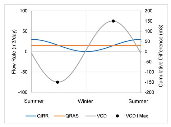
Figure 2.
Conceptual seasonal variation in water supply, demand and cumulative difference, for a recirculating aquaculture system discharging 15 m3 day−1.
Water management practices of effluent disposal and freshwater supplementation can also be used at times of maximum cumulative difference, to dispose of surplus effluent or supply deficit irrigation water [23,25,28]. Therefore, if the required infrastructure is available to deliver supplementary irrigation water or receive effluent, these practices can reduce overall storage requirements. Disposal and supplementation also impact the annual volume of water for irrigation, and therefore impact the size of the growing area and the reuse rate of the HRS. Considering targets for disposal and supplementation are therefore critical in the conceptual design of end-of-pipe HRS.
3. Materials and Methods
A two-step method was used to determine the critical requirements for feasible/viable end-of-pipe HRS, using two representative horticulture components: SOIL-FIELD, representing a low-cost, lower-return option, and HYDRO-GH, representing a higher-cost but higher-return option. The first step employed hydrologic modelling to size HRS components. Economic modelling was then used to assess economic viability of each HRS. Both systems used lettuce as a representative crop, grown in typical patterns for Australian climates. Simulations were run across a range of water management and climate scenarios, to assess their impact on the three critical requirements for feasibility/viability.
3.1. HRS Model Description
Two separate one-dimensional (1D) hydrologic models were developed for SOIL-FIELD and HYDRO-GH. Each model comprised a tank storage component and a horticulture component, as shown in Figure 3. The hydrologic models simulated water flows on a daily time step. The tank storage area () with fixed depth () and horticultural system growing area ( or ) variables were optimized to size each end-of-pipe HRS in various water management and climate scenarios. Total land required for the end-of-pipe HRS was calculated as the sum of the horticultural growing area of either system () and storage area (), multiplied by a factor of 1.1 to account for ancillary land uses, as in Equation (1).
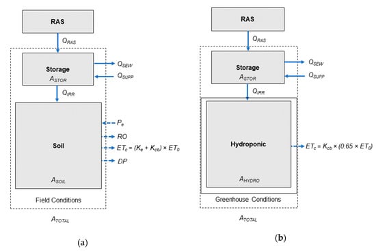
Figure 3.
End-of-pipe horticultural reuse scheme (HRS) hydrologic model for (a) SOIL-FIELD and (b) HYDRO-GH.
Economic parameters were also attributed to each component of the hydrologic model to assess economic viability. The models were developed in Microsoft Excel (2016), utilizing built-in functions, Solver and Goal Seek, controlled through visual basic for applications (VBA). Water balance model variables for SOIL-FIELD and HYDRO-GH are listed in Table A1, and model constants in Table A2, in Appendix A.
3.2. Recirculating Aquaculture System (RAS)
The effluent discharge from the RAS () was based on a hypothetical facility producing 45,000 kg/year with a stocking density of 50 kg/m3, discharging 5% total system water volume per day (15 m3/day). Effluent water quality parameters from a RAS facility in Warrnambool, Australia [49] were used to calculate sewer discharge costs. Any nutritional plant deficiencies in the wastewater were assumed to be supplemented using inorganic elements at an insignificant cost (approximately AUD 1/kg). Water quality was not modelled.
3.3. Storage Component
The storage water balance simulated the daily storage water volume () on day ‘i’, accounting for daily inflows of RAS effluent () and supplementary irrigation water (), and daily outflows of irrigation water () and sewer discharge (), as described in Equation (2). The model assumed no additional losses from the tank, i.e., no evaporation or leakage.
Storage volume () was calculated as a storage area () multiplied by fixed depth (). The initial simulation storage volume was 50% capacity (). For both end-of-pipe HRS models, effluent flows from RAS effluent inflow () to tank storage were assumed to be a constant daily flow rate. If the sum of RAS effluent inflow and effluent volume from the previous day () exceeded capacity, (), the excess effluent flowed to sewer for disposal (), as described in Equation (3). Sewer disposal, however, was constrained in each optimization scenario according to a maximum allowable discharge per year (), based on a targeted reuse fraction, i.e., a percentage of the annual RAS effluent. The difference in final tank storage volume was constrained to ±1 mL to prevent significant net storage or loss. Final storage () was equal to , where n equals the total length of the 10 year-long simulation (), equal to 3652 days.
Effluent flowed from the tank storage based on daily irrigation water demand (). If daily irrigation demand exceeded the volume of effluent in tank storage on the previous day () and the daily RAS inflow (), supplementary irrigation water flowed into the tank to meet the demand (), described in Equation (4). No evaporative loss is modelled for tank storage. Supplementary irrigation was also constrained in each optimization scenario according to a maximum annual volume ().
3.4. Horticulture System
Daily irrigation water demand () for SOIL-FIELD and HYDRO-GH were determined using specific irrigation water balance models, to represent the hydrological differences of each system.
3.4.1. SOIL-FIELD Water Balance
SOIL-FIELD used a detailed root zone water balance [Equation (5)], adopted from Chapter 8 of Allen et al. (1998), with capillary rise from groundwater omitted. The omission reflected the need to site end-of-pipe HRS with high nutrient RAS effluent away from areas with likely groundwater interactions. The water balance simulated root zone water depletion () on day ‘i’, accounting for effective rainfall (), runoff as overland flow (), irrigation (), crop water use () and deep percolation (), as shown in Figure 3.
Crop water use () was calculated using the dual crop coefficient method, which partitions daily soil evaporation () and crop transpiration ), with daily Penman–Monteith reference evapotranspiration (), as shown in Equation (6).
Soil evaporation () was limited by using a soil surface water balance, adopted from Chapter 7 of Allen et al. (1998). The soil surface water balance simulates soil surface depletion () on day ‘i’, accounting for the fraction of soil surface wetted by irrigation or precipitation (), the exposed (not under the crop canopy) and wetted soil fraction (), soil evaporation () and the deep percolation from the soil surface to the root zone (), as shown in Equation (7).
Daily SOIL-FIELD irrigation water demand () was equal to 0 if the root zone water depletion () was less than the threshold water content before plant moisture stress, or ‘readily available water’ (), and equal to multiplied by the growing area () if was greater than or equal to .
is calculated using the depletion fraction of total available water in the root zone before plant moisture stress (), field capacity (), wilting point () and root depth (), all of which vary for soil and crop types. See Chapter 7 and Chapter 8 of Allen et al. (1998) for further details on calculation methods for Equations (5)–(9).
3.4.2. HYDRO-GH Water Balance
HYDRO-GH used a simplified ‘single bucket’ model. No effective rainfall inflows () to the system were modelled due to the presence of a greenhouse covering, and no deep percolation () losses were modelled from the enclosed horticulture system, as shown in Figure 3. Daily hydroponic irrigation water demand () was determined based only on the crop water demand. The evaporation component for the crop coefficient () was excluded, to represent the negligible evaporation outflow from hydroponic systems. A greenhouse coefficient () was applied to account for the reduction in reference evapotranspiration inside the greenhouse, and a utilization coefficient ( ) to account for fraction of utilizable area, as shown in Equation (10).
Dumping of hydroponic solution, i.e., periodic exchange of the solution to manage salt accumulation, was neglected in this simplified water balance. It is noted that ‘exchange’ or ‘dumping’ of effluent volumes could significantly impact annual hydroponic irrigation water demand (), particularly affecting systems without treatment devices that enable solution reuse, e.g., desalination.
3.4.3. Horticulture Model
To determine daily for either horticulture system, a model crop type and cropping schedule was required. Lettuce was selected as the crop type used in both systems. A representative cropping schedule was designed, using basal crop coefficients () for the various crop stages across a 365 day period. While crop rotation is common practice, for modelling purposes the same crop type was considered suitable, as similar crops to lettuce (leafy greens) are best suited to RAS effluent. Basal crop coefficients and stage lengths for lettuce were selected using Table 17 in Allen et al. [44], directly input for SOIL-FIELD and adjusted for HYDRO-GH. HYDRO-GH was reduced by 10% for , and 17% for both and , using plastic mulch values in Table 25 from Allen et al. [44], to account for reduction due to hydroponic production, similar to the method used in Goddek et al. [20].
SOIL-FIELD was assumed to produce three crops annually in a single plot. Crop lengths varied from a minimum of 75 days in summer to a maximum of 105 days in winter (refer to Table A3 and Table A4). Plant density used was 8 plants/m2. Annual SOIL-FIELD yield was modelled as 9.03 kg/m2, consistent with published values [50].
HYDRO-GH was assumed to produce six crops annually in three subplots, with planting staggered one week apart. Crop lengths varied from 35 days in summer to 91 days in autumn/winter (refer to Table A3 and Table A4). Plant density used was 20 plants/m2. Annual HYDRO-GH yield was modelled as 27.5 kg/m2, based on previous unpublished experiments using RAS effluent in HYDRO-GH conditions. Modelled annual yield in HYDRO-GH was lower than the 41 kg/m2 for hydroponic lettuce in Arizona in [39], as no artificial heating or lighting was expected in the lower technology greenhouse modelled in this study.
3.5. Economic Model
The economic model estimated profitability of each end-of-pipe HRS at an annual time step. It used input data from Australian horticultural studies and government statistics, shown in Table A5. The economic model calculated total aggregate profit () in each end-of-pipe HRS scheme as the sum of the annual (year ‘i’) differences between revenue () and operating cost (), as shown in Equation (11) using constant values presented in Table A6. Annual revenue and operating costs were constant for the simulated period in this study. In the following sections, the subscript ‘hort’ represents parameters that are specific to either of the horticulture systems in SOIL-FIELD and HYDRO-GH models.
Annual revenue () was calculated as the annual yield (), accounting for the fraction of crop loss () multiplied by the crop price (), as in Equation (12).
Operating costs () for either system were calculated as the sum of the horticulture operating costs per unit area () for the total horticulture area (), total sewer costs () for the annual volume (), total supplementary water costs () for annual volume (), and pumping costs (), as in Equation (13).
The internal rate of return () for the end-of-pipe HRS was calculated as the discount rate at which the net present value () of the end-of-pipe HRS was equal to zero. The over the simulation period in years was calculated as the capital cost of the scheme () minus the sum of annual profits.
Capital costs were calculated as the sum of the unit area capital cost of tank storage () multiplied by the total storage area (), the unit area capital cost of the horticulture system () multiplied by the growing area (), and the unit area cost of land () multiplied by the total land area ().
3.6. Modelling Methods
The modelling process was carried out in two parts, as shown in the modelling procedure below. All calculations were performed in Microsoft Excel, using linear programming/optimization add-in Solver, iteration add-in Goal Seek, and VBA programming language to automate routines. Constraints used to define specific hydrological and economic objectives for optimization routines, used across the water management and climate scenarios, are presented in Table 1 and Table 2.

Table 1.
Optimization constraints (all $ values in AUD).
Table 2.
Water management scenarios.
3.6.1. Modelling Procedure
Part 1—Sizing and feasibility assessment
- 1.
- Determine the average RAS effluent inflow at a daily time step ().
- 2.
- Determine a representative crop type, cropping pattern and yield over a 365 day period for each horticulture system. The cropping pattern requires a list of crop coefficient (Kc) values for the selected crop type each day of the 365 day period, that should reflect local growing periods. Multiply the 365 day period by the years required for the length of simulation. It was assumed that 5–10 years should account for climatic variation.
- 3.
- Collate representative climate data (ET0 and rainfall) at a daily time step for a representative period equal to the length of the simulation.
- 4.
- Select the annual allowance for effluent disposal, supplementary irrigation and other optimization constraints, as shown in Table 1, for each conceptual design.
- 5.
- Define all variables and constants in the irrigation water balance for the horticulture system [Equations (2)–(10)].
- 6.
- Use linear programming/optimization (e.g., MS Excel’s Solver) to minimize storage area over a defined simulation period (5–10 years), with storage area and growing area as the two decision variables and constraints, as shown in Table 1.
- 7.
- Use Equation (1) to determine total land requirement.
Part 2—Capital costs, crop price and viability assessment
- 8.
- Input estimates for capital cost (land, tank and growing area) and operational/production costs (production cost, disposal and supplementary water costs).
- 9.
- Use total land areas to calculate end-of-pipe HRS total capital expenditure.
- 10.
- Select target internal rate of return (IRR) over the life of the scheme.
- 11.
- Use iteration (e.g., MS Excel’s Goal Seek) on crop price to achieve the target IRR.
- 12.
- Assess feasibility/viability of each conceptual design based on the critical requirements, total land, capital expenditure and access to markets with demand for required crop prices.
Steps 1–12 can be repeated using different horticulture systems, crop types, and annual sewer and supplementary irrigation allowances, to assess feasibility and viability of alternative end-of-pipe HRS designs and scenarios.
3.6.2. Modelled Scenarios
The climate scenarios represent four different Australian climates, with Köppen classifications for each shown in Table 3 below, and statistics in Table 4. The climate scenarios were selected to assess the impact of climate, specifically rainfall and evapotranspiration (ET0), on the critical requirements for HRS. Adelaide (Parafield) represented a base case, Adelaide (Mt Lofty) a wetter climate with lower ET0, Hobart as a similar rainfall and lower ET0, and Darwin with high ET0 and high annual rainfall. Daily weather data sets were used for the four climate scenarios for the period 1 January 2009 to 31 December 2018. Mean monthly values for each climate/location are presented in in Figure 4 and mean annual values for the simulation in Figure 5.
Table 3.
Climate scenarios and Köppen classification.
Table 4.
Climate parameters for modelled locations from historical data set, 2009–2018 [51].
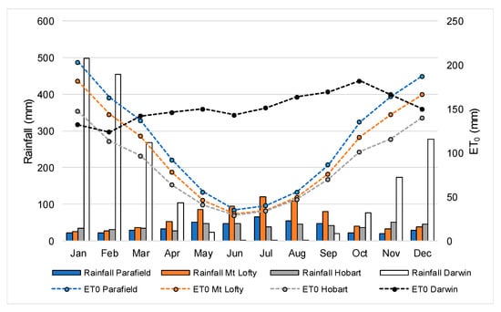
Figure 4.
Mean monthly rainfall and reference evapotranspiration (ET0) for each climate scenario, climate data from Bureau of Meteorology [51].
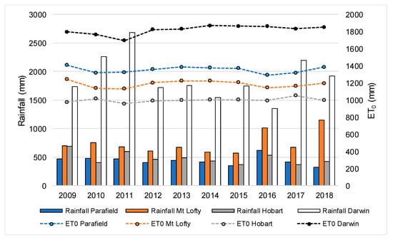
Figure 5.
Annual total rainfall and reference evapotranspiration (ET0) for each climate scenario, climate data from Bureau of Meteorology [51].
3.7. Verification and Sensitivity Analysis
Outputs from the irrigation water balance models were verified by checking water use statistics for lettuce crops in soil-based systems in field conditions, and hydroponic systems in greenhouse conditions. Crop prices were verified against listed wholesale prices. Sensitivity analysis was conducted on crop water use in the hydrologic model by adjusting Kc by ±10%, to assess the model uncertainty related to hydrologic inputs (Scenario 12 and 13). Sensitivity analysis was also conducted on production costs, capital costs, land costs, storage costs, sewer disposal cost and supplementary water cost, to assess their contribution to model uncertainty. To test sensitivity, the inputs were individually adjusted by ±10%. The optimization and ‘goal seek’ routine was rerun for crop water use inputs, but only the ‘goal seek’ routine was rerun for the other economic inputs. Outputs from adjusted models were compared against the unadjusted results.
4. Results
4.1. Adelaide (Parafield)
Comparing results for SOIL-FIELD against HYDRO-GH in Parafield shows the impact of horticulture system type on end-of-pipe HRS land and capital expenditure requirements. SOIL-FIELD (Figure 6) requires significantly less land and less capital expenditure than HYDRO-GH (Figure 7) in all water management scenarios (1 to 13). Total reuse with no sewer disposal or supplementary irrigation (Scenario 1) in HYDRO-GH requires approximately 3 times more land (21,963 m2) compared to SOIL-FIELD (7421 m2), and 13.9 times more capital expenditure (AUD 2636 k (‘000) compared to AUD 189 k). To achieve a typical rate of return of 3.6% for SOIL-FIELD, and 11.0% for HYDRO-GH, over a 10 year period, SOIL-FIELD requires a target crop price of AUD 1.57 per kg, compared to AUD 7.66 per kg in HYDRO-GH, as shown in the tables adjacent to the graphs in Figure 6 and Figure 7, respectively. The storage percentage shown is presented as a fraction of the total annual RAS effluent volume discharged, i.e., 5.48 mL/y.
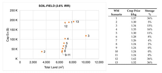
Figure 6.
Soil-based system in field conditions (SOIL-FIELD) results for Adelaide (Parafield) climate.
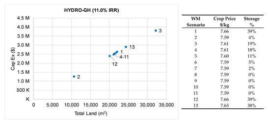
Figure 7.
Hydroponic system in greenhouse conditions (HYDRO-GH) results for Adelaide (Parafield) climate.
Disposing of 50% of the annual RAS wastewater load to sewer (Scenario 2) approximately halved the land requirement in both SOIL-FIELD and HYDRO-GH, reduced capital expenditure by 80% in SOIL-FIELD and 53% in HYDRO-GH. The 50% sewer allowance also saw storage volumes, as a fraction of the annual RAS wastewater load, drop from 36% (2.0 mL) in SOIL-FIELD and 39% (2.1 mL) in HYDRO-GH in Scenario 1, to 4% (0.22 mL) and 5% (0.27 mL), respectively in Scenario 2. The greater reduction in SOIL-FIELD capital expenditure was due to the relative cost of storage per unit area (AUD 80.00) compared to capital costs for the SOIL-FIELD horticulture system ($3.20), as well as disposal being relatively cheap (AUD 0.19/m3). The breakdown of capital expenditure for SOIL-FIELD and HYDRO-GH, shown in Figure 8 and Figure 9 respectively, explains the relative costs for components of the two end-of-pipe HRS across the 13 water management scenarios.
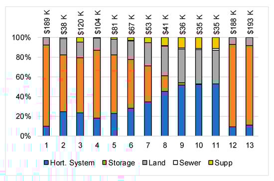
Figure 8.
Capital expenditure breakdown for soil-based system in field conditions (SOIL-FIELD) in Parafield climate (K = ‘000).
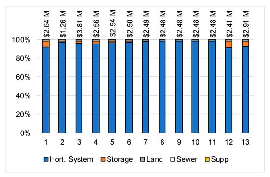
Figure 9.
Capital expenditure breakdown for hydroponic systems in greenhouse conditions (HYDRO-GH) in Parafield climate (M = ‘000,000).
The substantial reduction in SOIL-FIELD capital cost in Scenario 2 also had a positive impact on SOIL-FIELD viability, lowering the required crop price by 8% from AUD 1.57 to AUD 1.30 per kg. A much smaller impact was observed in HYDRO-GH, reducing from AUD 7.66 to AUD 7.59 per kg (less than 1%), due to the much higher capital costs per unit area (AUD 127.43).
Allowing an annual supplementary irrigation volume equal to 50% of the annual RAS effluent volume (Scenario 3 in Figure 6 and Figure 7) reduced required storage to 15% in SOIL-FIELD, and 19% in HYDRO-GH. However, this was at the cost of 35% more land, due to increased growing areas to consume the additional water volumes. Increased growing area and reduced storage reduced capital costs by 47% in SOIL-FIELD, but increased them in HYDRO-GH by 33%, due to the different storage cost to horticulture system capital cost ratios, as described above.
Combining sewer disposal with supplementary irrigation volumes significantly reduced the storage requirement, by enabling disposal in surplus periods and supplementation in deficient periods. Relaxing model constraints to allow annual sewer disposal and supplementary irrigation volumes up to 6.25% of the annual RAS effluent volume each (Scenario 4) significantly reduced the storage volume in both systems. The storage fraction dropped from 36% in SOIL-FIELD and 39% in HYDRO-GH for Scenario 1, to 16% (0.88 mL) and 19% (1.0 mL), respectively, for Scenario 4.
Water balances for SOIL-FIELD and HYDRO-GH define the percentage mean annual inflows and outflows for each horticulture system, which are constant for all Parafield scenarios. For SOIL-FIELD, Figure 10a shows the distribution of inflows and outflows, showing additional rainfall inflows are more than accounted for by additional losses from the horticulture system (soil evaporation, deep percolation, interception and runoff/overland flow). For HYDRO-GH, the water balance is 100% effluent irrigation inflow and 100% transpiration outflow, as shown in Figure 10b.
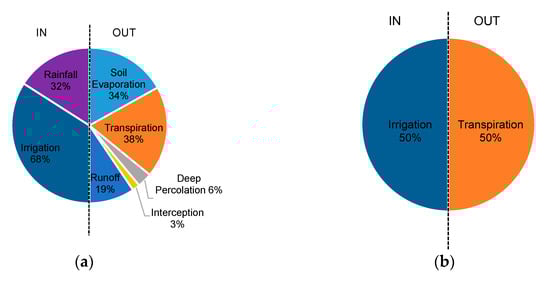
Figure 10.
(a) Annual soil-based system in field conditions (SOIL-FIELD) water balance for the ten year simulation in Adelaide (Parafield) climate; (b) Annual hydroponic system in greenhouse condition (HYDRO-GH) water balance for the ten year simulation in Adelaide (Parafield) climate.
Analysis of the cumulative difference between RAS effluent supply and irrigation demand over the simulation (Figure 11) shows the impact of different crop patterns in SOIL-FIELD and HYDRO-GH Scenario 1 (full reuse). A divergence becomes apparent around 2015, leading to a difference of approximately 1.0 mL by the end of the simulation, −230 kL for SOIL-FIELD and 763 kL for HYDRO-GH; both within the ±1.0 mL from the initial volume model constraint.
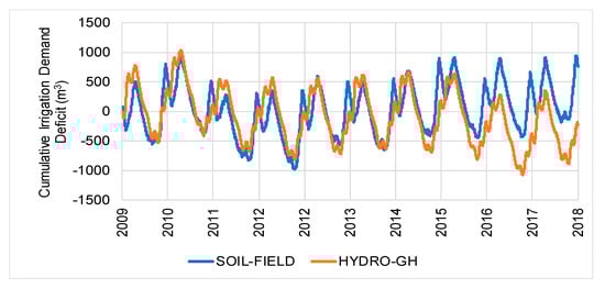
Figure 11.
Cumulative difference (VCD) between recirculating aquaculture system effluent supply and irrigation demand in SOIL-FIELD and HYDRO-GH for Parafield climate, Scenario 1 over the ten year simulation.
Sensitivity analysis in Scenario 12 (+10% irrigation demand) and Scenario 13 (−10% irrigation demand) in Figure 6 and Figure 7 show the model uncertainty attributed to irrigation demand. Scenario 12 and 13 show directly proportional increases in total land (i.e., ±10%) for both SOIL-FIELD and HYDRO-GH when compared to Scenario 1, with negligible change to capital expenditure in the SOIL-FIELD. Impacts to capital expenditure in HYDRO-GH, however, were significant, due to the changes to irrigation demand, increasing by approximately AUD 100 k in Scenario 12 and decreasing by the same amount in Scenario 13. Sensitivity analysis of economic input parameters in Table 5 and Table 6 show that in both SOIL-FIELD and HYDRO-GH, production costs had the most significant impact on required crop prices, followed by storage cost in SOIL-FIELD, and capital costs in HYDRO-GH. Less than proportional changes to model outputs in Scenarios 12 and 13, and the economic sensitivity analysis, suggests the water balance and economic models are relatively stable, with respect to the uncertainty of these parameters.
Table 5.
Sensitivity analysis of SOIL-FIELD crop price to changes in economic inputs.
Table 6.
Sensitivity of HYDRO-GH crop price to changes in economic inputs.
4.2. Climate Scenarios
4.2.1. SOIL-FIELD
SOIL-FIELD results for the four climate scenarios in Figure 12 show significant variation in required land and storage, and therefore capital expenditure and crop price. Hobart required the largest land area (9141 m2) for total reuse (Scenario 1), while Darwin required the smallest land area (5372 m2). Capital expenditure for full reuse (Scenario 1) in each climate ranged between AUD 150 K (‘000) and AUD 190 K for Hobart, Parafield and Darwin, while Mt Lofty was higher, at AUD 231 K, due to a greater storage requirement of 44% (2.4 megaliters, ML). Crop prices in SOIL-FIELD reflect the ratio of growing area to storage volume, being highest in Darwin Scenario 1 (AUD 1.84/kg) and lowest in Hobart Scenario 11 (AUD 1.20/kg). Darwin and Hobart responded best to a 50% supplementary irrigation allowance (Scenario 3), seeing reductions in storage requirements of approximately two thirds, while Parafield and Mt Lofty storage volumes were approximately halved. Combined sewer and supplementary irrigation allowances, each of 50% of the annual RAS volumes (Scenario 11), eliminated the need for storage in all modelled climates. The crop price for Hobart in Scenario 11 is the lowest of all modelled scenarios, due to it having the largest growing area, and therefore valuable yield to overcome disposal and supplementary costs.
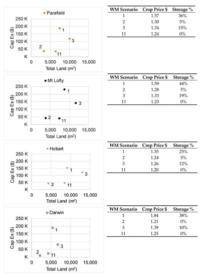
Figure 12.
Soil-based reuse in field conditions (SOIL-FIELD) across four Australian climates.
4.2.2. HYDRO-GH
HYDRO-GH results in Figure 13 also shows significant variation in land and capital expenditure requirements between climates. Unlike SOIL-FIELD, however, rainfall did not impact system hydrology in greenhouse conditions, leaving evapotranspiration as the sole variable determining land requirement between climates. Land area was therefore inversely proportional to evapotranspiration over the simulated period. For full reuse (Scenario 1), Darwin had the smallest land requirement (15,998 m2), followed by Parafield (21,963 m2), Mt Lofty (24,878 m2), and Hobart with the greatest (29,420 m2). In scenario 1, storage requirements for HYDRO-GH were similar to those for SOIL-FIELD, increasing for Parafield (+3%) and Hobart (+8%), but decreasing for Mt Lofty (−4%) and Darwin (−6%). As found in SOIL-FIELD, Darwin required the smallest sewer and supplementary irrigation allowance to eliminate the need for storage—25% compared to 31% for all other climates—which reflects lesser seasonal variation in Darwin ET0 (see Figure 2 and Figure 4).
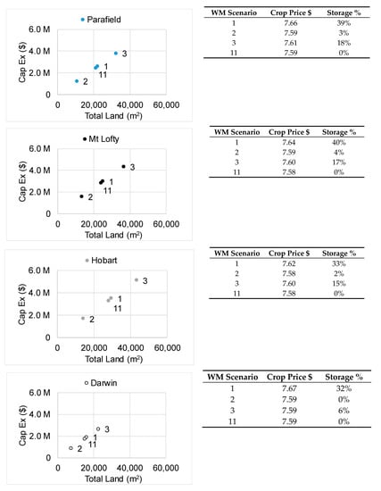
Figure 13.
Hydroponic reuse in greenhouse conditions (HYDRO-GH) across four Australian climates.
5. Discussion
5.1. Water Use and Land Requirement
As a result of reduced irrigation water demand, HYDRO-GH systems are more land intensive than SOIL-FIELD systems in all water management and climate scenarios. This is counterintuitive for locations with high annual rainfall, like Darwin, which receives an average of 1893 mm added to the SOIL-FIELD water balance annually. Water balance analysis, however, shows that most of the rainfall (+34%) in SOIL-FIELD is likely lost through runoff/overland flow (−19%) (using the United States Department of Agriculture (USDA) Soil Conservation Service curve number method for agricultural lands), deep percolation (−6%), and interception (−3%), as shown in Figure 10. As a result of the high rainfall losses, crop evapotranspiration (ETC) plays a greater role than rainfall in the sizing of SOIL-FIELD in the modelled climates. ETC is higher in SOIL-FIELD relative to HYDRO-GH, due to reductions experienced in HYDRO-GH from both protected cropping conditions and the use of the hydroponic system. Protected cropping reduces solar radiation and wind speed, and increases humidity at the plant level, unless artificial lighting or heating is employed, accounting for a 35% reduction in ET0 [52] as modelled in this study. The hydroponic system effectively eliminates growing surface evaporation (Ke), accounting for a 10% to 30% reduction in Kc [44]. Combining reduced ET0 and Ke results in an ETC reduction of approximately 72% for the same crop type. Barbosa et al. [39] compared annual water use between soil-based field and hydroponic greenhouse lettuce production in Arizona, USA, using 250 L/kg/year for flood irrigation in the SOIL-FIELD system, and 20 L/kg/year for HYDRO-GH system. Using the values in Barbosa et al. [39] with yields from this study gives a difference of 4.1 times the irrigation demand in SOIL-FIELD compared to HYDRO-GH. This is approximately 16% higher than the average value of 3.4 for SOIL-FIELD and HYDRO-GH in this study, which could be attributed to higher irrigation application rates using flood irrigation compared to the drip irrigation method modelled here in SOIL-FIELD. In this study, the benefits of greater water use efficiency for HYDRO-GH, therefore, come at the cost of significantly greater land requirements in an end-of-pipe HRS using HYDRO-GH. A greater land requirement for HYDRO-GH could mean such systems are not feasible in situations where land is constrained, however, HYDRO-GH can be suitable/feasible on non-arable soil. Therefore, where land is not constrained and is considered non-arable, HYDRO-GH may be the only feasible solution. Hydroponic systems in field conditions may be able to achieve greater water use efficiency than soil-based systems, at a lower cost than HYDRO-GH modelled in this study, due to savings without the greenhouse capital cost, such as those commonly used in Virginia, South Australia and Almeria, Spain.
Comparing results for the hydroponic system in scenario 1 (100% reuse)—Parafield (21,963 m2 at 34.8° S), Mt Lofty (24,878 m2 at 35.0° S), Hobart (29,420 m2 at 42.8° S) and Darwin (15,988 m2 at 12.4° S)—with results in Goddek and Korner [21] for an equally sized 45,000 kg per year RAS in Namibia (9250 m2 at 22.6° S), The Netherlands (14,000 m2 at 52.0° N) and Faroe Islands (15,750 m2 at 66.0° N), suggests growing areas in this study were greater than those in Goddek and Korner. This may reflect the use of a nutrient balance design approach used in Goddek and Korner, as well as other assumptions about plant water use and the cropping environment that differ to this study. Greater land area requirements for locations with lower evapotranspiration in Goddek and Korner support the same findings in this study.
5.2. Storage
The minimum storage requirement for a fixed area 100% reuse system should be equal to the maximum absolute cumulative difference () between effluent supply (QRAS) and irrigation demand (QIRR) over a given period, as shown in Figure 2. Any factor that increases will increase the required storage volume, and vice versa. As such, it could be expected that the protected cropping conditions for HYDRO-GH would reduce the storage requirement by eliminating winter rainfall. For Parafield, Mt Lofty and Hobart climates, most rainfall occurs in winter during periods of low irrigation demand. Modelling results, however, show no substantial difference in storage requirements between SOIL-FIELD and HYDRO-GH in these three climate scenarios. Annual water balance analysis (Figure 10) shows that the soil evaporation not experienced in HYDRO-GH more than accounts for rainfall minus runoff/overland flow at an annual timescale. More significant to storage requirement, perhaps, is scheduling crops so that Kcmax does not coincide with ET0 max or, to a lesser extent, a fallow period does not occur during ET0 min. Figure 11 shows the impact of Kc max for SOIL-FIELD coinciding with a period of very high ET0 in 2015, causing the distinct divergence in cumulative differences between the two systems experiencing the same ET0, since HYDRO-GH has a different cropping schedule. It can be expected that little difference in the storage requirement between systems such as SOIL-FIELD and HYDRO-GH will be experienced when growing the same crop with the same cropping schedule, although if the simulation was extended there may be differences in storage requirements, as a result of the divergence caused by Kcmax in SOIL-FIELD coinciding with very high ET0. Measures like staggered plantings or continuous harvesting would reduce the between irrigation water demand and RAS effluent supply, which is common practice in many commercial horticulture systems. Higher technology greenhouses would also be able to better regulate irrigation water demand, and therefore reduce , and reduce/eliminate the need for storage in HYDRO-GH. However, this is expected to be at greater capital expenditure, and significantly greater operational cost, than those assumed for HYDRO-GH in this study. Considering that poor water quality impacts are likely to occur if high nutrient RAS effluent was exposed to sunlight, pond storage was not considered in this study. In arid climates, storage ponds are net water disposers per year, and with sufficient depth could be neutral in tropical climates, like Darwin. If water quality was managed in pond storage, the growing area could be reduced through the evaporative disposal mechanism. The dynamics of rainfall and evaporation over the storage area, however, would need to be added to the storage water balance [Equation (2)]. At the time of writing there is a lack of studies to compare storage volumes for each climate, although prescriptive guidelines are available for alternative sizing methods [53].
5.3. Water Management
Disposal and supplementation of irrigation water in surplus and deficit periods can reduce the peaks and troughs of the absolute cumulative difference () between effluent supply (QRAS) and demand (QIRR). This was shown to substantially reduce storage requirements in both systems in all climates. Darwin SOIL-FIELD and HYDRO-GH required the smallest sewer and supplementary allowance to eliminate storage, which reflected smaller peaks and troughs in the (), due to less seasonal ET0 variation (Figure 2). Practically, effluent could be discharged via sewer (considered more likely in urban and peri-urban locations), via environmental discharge in rural locations (so long as the required environmental approvals can be obtained), and via existing evaporation ponds or to adjacent available pasture in rural zones. In detailed end-of-pipe HRS design, the cost of discharge should reflect actual costs, but for the purpose of this study, disposal costs were assumed to equal sewer disposal costs.
An alternative to disposal or supplementation would be to vary the size of the growing areas with seasons: expanding the growing area during low ET0 periods, and contracting in high ET0 periods. A seasonally varying growing area would be suited to scenarios where land is not constrained, or where other users are available to receive effluent during surplus periods. This is commonly practiced by local councils in Australia that have irrigation networks connecting multiple sports fields to sewage plant effluent ponds [54,55].
Flexibility is an important component of a profitable HRS. Operators of an end-of-pipe HRS would need to be able to adapt to changes in RAS effluent water quality and supply, weather, and markets for crops, in order to achieve best performance. This might involve changing crop types and crop schedules, which ultimately impacts irrigation demand and storage volumes. Access to disposal and supplementary irrigation would enable such flexibility, and would therefore be an important component of a HRS.
5.4. Capital Expenditure
As well as being land intensive, HYDRO-GH is also very capital intensive. HYDRO-GH requires approximately 14 times more capital expenditure than SOIL-FIELD to consume the total annual volume of RAS effluent. HYDRO-GH is therefore unlikely to be feasible/viable where either land or capital is constrained. For an existing RAS, it is likely that the initial capital expenditure of a HYDRO-GH end-of-pipe HRS designed for 100% reuse would be greater than that of the RAS itself. Like in aquaponics systems, this would see an integrated RAS-horticulture business producing majority plant products. Considering these findings, integrating an existing RAS with a HYDRO-GH might only occur where a horticulturalist is seeking an alternative water source for their sizeable horticulture business, or if only partial reuse was practiced, e.g., 50% or 25% of the annual RAS wastewater load.
SOIL-FIELD appears likely to be feasible/viable in more situations than HYDRO-GH, due to its lower land and capital requirements. Storage reductions achieved in SOIL-FIELD through disposal and supplementation also have a much more significant impact on capital expenditure, whereas these are insignificant in HYDRO-GH. Sensitivity analysis in Table 5 shows that SOIL-FIELD is more sensitive to the cost of disposal or supplementation than HYDRO-GH (Table 6), however this would have to increase substantially for the economic benefit of either practice to be eliminated. Therefore, so long as sewer and supplementary costs are reasonable, SOIL-FIELD should be more feasible/viable than HYDRO-GH in most situations, although with a lower rate of return on investment expected in SOIL-FIELD (modelled as 3.6% compared to 11% for HYDRO-GH in this study).
5.5. Crop Price
Crop prices in Figure 12 and Figure 13 reflect the profitability required to overcome capital expenditure costs from the growing area and storage tanks, based on a target IRR. The reductions in capital expenditure and crop price in SOIL-FIELD, occurring as a result of reduced storage requirements (e.g., Figure 12, Hobart Scenario 1 versus 11), suggest that accurately sizing storage components for lower intensity horticulture systems will be crucial to maximizing financial returns. Since HYDRO-GH growing area is so capital intensive, little variation in crop price is observed across all scenarios, regardless of storage reductions. Actual crop prices required in HYDRO-GH correspond to high value crops such as brussels sprout (AUD 7.50/kg) and birds eye chili (AUD 9.41/kg) [56], while actual prices required in SOIL-FIELD correspond to lower value crops, such as lettuce (AUD 1.35/kg) and broccoli (AUD 1.54/kg) [37]. Therefore, for HYDRO-GH to be viable, access to high value markets is essential. Changing the target IRR would impact the required crop price of an HRS, which may be significantly higher in some HYDRO-GH scenarios (up to 25% based on industry estimates [57]), and may require higher value crops, such as herbs (>AUD 10/kg). Different yields to those modelled here, as a result of different crops, cropping practices or weather impacts, would also impact the required crop price. Therefore, estimates on marketable yields for any end-of-pipe HRS should be conservative at the feasibility assessment stage.
5.6. Climates
Results from Darwin suggest locations at lower latitudes closer to the equator, with consistent and high irrigation demand, will require the least land and capital, making them more likely to be feasible, assuming lettuce or crops with similar irrigation demand can be grown year-round. Reuse is more land intensive in cooler climates with lower irrigation demand, such as in Hobart. Therefore, existing RAS at higher latitudes, including locations where salmon smolts are farmed, would require significantly more land, with greater storage requirements incurred for shorter growing seasons, unless disposal of a significant fraction of the effluent load is feasible.
5.7. Application and Limitations
The method developed in this study to compare SOIL-FIELD and HYDRO-GH represents a novel approach to feasibility/viability assessment of end-of-pipe HRS. The modelling method focused on sizing end-of-pipe HRS to minimize storage costs and achieve specific reuse objectives, i.e., full or partial reuse. The modelling methods quantified three critical requirements (‘ingredients’) for end-of-pipe HRS investors: total land, capital expenditure and crop price. Applications of this type of sizing and assessment method could range well beyond RAS effluent reuse. Examples could include small-scale applications, such as sizing of rainwater tanks for community gardens, through to large-scale urban and peri-urban irrigation reuse schemes, for municipal effluent or industrial wastewater. The ‘ingredients’ approach to viability assessment also creates a simple framework for providing subsidies, to incentivize end-of-pipe HRS where it is not currently viable but would provide environmental and other socio-economic benefits, in line with integrated water management principles.
There are several limitations in the modelling method used in this study. The use of a single crop type (lettuce) did not capture the impacts of varying crop irrigation water demands. Using other crops would likely impact the required land, storage, capital expenditure and crop prices, all of which are shown to have a directly proportional relationship to land requirements, as demonstrated in Scenario 11 and 12. Different irrigation practices would also impact irrigation water demand, as would location-specific growing seasons that better reflect each climate scenario (e.g., Darwin may be too hot to grow lettuce year-round), rather than the single schedule used for each horticulture system in this study. Actual capital expenditure and crop prices used in this study serve as a guide and show relative changes across different scenarios. A more detailed assessment of feasibility and viability in any location would be expected to include land values, specific crop types, cropping patterns and yields that more precisely represent that crop type, cultivar and a nutrient balance.
6. Conclusions
When compared to the soil-based system in field conditions, the hydroponic system in mid-tech greenhouse conditions substantially increased the total land requirement and capital expenditure of a feasible/viable horticultural reuse scheme. As a result, hydroponic systems in greenhouse conditions require production of, and markets for, high value crops. Despite different hydrological characteristics, the hydroponic system modelled in this study required similar effluent storage volumes to the soil-based system in field conditions; between 25% and 44% of the annual effluent volume for 100% reuse when using tanks. Small and targeted effluent disposal and supplementation can significantly reduce storage requirements, and substantially improve viability of soil-based HRS for RAS effluent. Finally, climates with high evapotranspiration substantially reduce the total land requirement, which may make 100% reuse HRSs for RAS effluent more feasible/viable in those locations.
Author Contributions
Conceptualization, E.M. and J.W.; Formal analysis, E.M.; Investigation, E.M.; Methodology, E.M. and J.W.; Project administration, J.W.; Resources, J.W.; Software, E.M. and J.W.; Supervision, J.W., W.L.; Visualization, E.M.; Writing—original draft, E.M.; Writing—review & editing, J.W., W.L. All authors have read and agreed to the published version of the manuscript.
Funding
This research was enable by funding through the South Australian Government Catalyst Research Grant with co-investment form the University of South Australia, with additional and direct research funding and in-kind support from the City of Salisbury.
Acknowledgments
Thanks to Michael Titley for his expert advice on lettuce production in Australia and the University of South Australia for funding the publication.
Conflicts of Interest
The authors declare no conflict of interest.
Abbreviations
| ET0 | reference evapotranspiration |
| HRS | horticultural reuse scheme |
| HYDRO-GH | hydroponic systems in greenhouse conditions |
| IAAS | integrated agri-aquaculture systems |
| IRR | internal rate of return |
| Kc | crop coefficient |
| Ke | evaporation component of the dual crop coefficient (Kc = Ke + Kcb) |
| Kcb | basal crop component of the dual crop coefficient (Kc = Ke + Kcb) |
| RAS | recirculating aquaculture system |
| SOIL-FIELD | soil-based system in field conditions |
Appendix A. Modelling Inputs
Table A1.
Water balance model variables.
Table A1.
Water balance model variables.
| Component | Parameter | Units | Description |
|---|---|---|---|
| Storage | m3 | Storage volume | |
| Storage | m3 | Storage volume on day ‘i’ | |
| Storage | m3 | Final storage volume | |
| Storage | m2 | Tank storage area | |
| Storage | m3 day−1 | Daily sewer discharge outflow | |
| Storage | m3 day−1 | Daily supplementary irrigation inflow | |
| Storage | m3 day−1 | Daily irrigation demand | |
| SOIL-FIELD | mm | Root zone depletion at end of day ‘i’ | |
| SOIL-FIELD | mm | Root zone depletion at end of previous day | |
| SOIL-FIELD | mm day−1 | Daily effective precipitation | |
| SOIL-FIELD | mm day−1 | Calculated using SCS curve number method [58], CN = 78 | |
| SOIL-FIELD | mm | Net irrigation on day ‘i’ that infiltrates the soil | |
| SOIL-FIELD | mm | Crop evapotranspiration on day ‘i’ | |
| SOIL-FIELD | mm | Deep percolation from root zone on day ‘i’ | |
| SOIL-FIELD | m2 | Soil system growing area | |
| SOIL-FIELD | mm | Readily available water | |
| SOIL-FIELD | m | Root zone depth (0.1–0.4) for lettuce | |
| SOIL-FIELD | - | Evaporation calculated as in Chapter 7 [44] | |
| SOIL-FIELD | mm | Soil surface zone depletion | |
| SOIL-FIELD | - | Fraction wetted | |
| SOIL-FIELD | - | Fraction wetted and exposed | |
| SOIL-FIELD | mm | Soil surface zone depletion | |
| SOIL-FIELD/HYDRO-GH | - | Basal crop coefficient (See Table A3 and Table A4) | |
| SOIL-FIELD/HYDRO-GH | mm day−1 | Reference evapotranspiration | |
| HYDRO-GH | m2 | Hydroponic system growing area |
Table A2.
Water balance model constants.
Table A2.
Water balance model constants.
| Component | Parameter | Units | Value | Description |
|---|---|---|---|---|
| HRS | days | 3652 | Simulation period (ten years) | |
| RAS | m3 day−1 | 15 | RAS inflow | |
| Storage | m | 2.25 | Tank depth | |
| SOIL-FIELD | mm | 48 | Total available water | |
| SOIL-FIELD | m3/m3 | 0.23 | Field capacity | |
| SOIL-FIELD | m3/m3 | 0.11 | Wilting point | |
| SOIL-FIELD | - | 0.3 | Depletion before water stress | |
| SOIL-FIELD | - | 0.3 | Fraction wetted by drip irrigation | |
| HYDRO-GH | - | 0.65 | Greenhouse coefficient [52] | |
| HYDRO-GH | - | 0.84 | Greenhouse utilization coefficient [36] |
Table A3.
Basal crop coefficients and lengths for lettuce crop stage lettuce crops in soil-based (SOIL-FIELD) and hydroponic greenhouse (HYDRO-GH) systems, adapted from [16,26].
Table A3.
Basal crop coefficients and lengths for lettuce crop stage lettuce crops in soil-based (SOIL-FIELD) and hydroponic greenhouse (HYDRO-GH) systems, adapted from [16,26].
| Crop Stage | Basal Crop Coefficient (Kcb) | Base Stage Length (Days) | ||
|---|---|---|---|---|
| SOIL-FIELD | HYDRO-GH | SOIL-FIELD | HYDRO-GH | |
| 0.15 | 0.14 | 20 | 10.0 | |
| - | - | 30 | 13.3 | |
| 0.90 | 0.75 | 15 | 8.3 | |
| 0.90 | 0.75 | 10 | 3.3 | |
| TOTAL | - | - | 75 | 35 |
Table A4.
Crop stage length multiplier to generate daily Kcb for a 365-day period.
Table A4.
Crop stage length multiplier to generate daily Kcb for a 365-day period.
| Crop No. | Multiplier for Base Stage Length | |
|---|---|---|
| SOIL-FIELD | HYDRO-GH | |
| 1 | 1.0 | 1.3 |
| 2 | 2.0 | 1.6 |
| 3 | 1.0 | 2.6 |
| 4 | - | 1.6 |
| 5 | - | 1.3 |
| 6 | - | 1.0 |
Table A5.
Economic model variables not included in the hydrologic models.
Table A5.
Economic model variables not included in the hydrologic models.
| Component | Parameter | Units | Description |
|---|---|---|---|
| HRS | $/yr | Annual profit | |
| HRS | $/yr | Annual revenue | |
| HRS | $/yr | Operating costs for each horticulture system | |
| HRS | $/kg | Required crop price to achieve IRR | |
| HRS | $ | Net present value of the HRS | |
| HRS | % | Internal rate or return | |
| HRS | $ | HRS capital cost |
Table A6.
Economic model constants (All $ values in AUD).
Table A6.
Economic model constants (All $ values in AUD).
| Component | Parameter | Description | Value | Units | Reference |
|---|---|---|---|---|---|
| HRS | Simulation period | 10 | years | - | |
| HRS | Cost of land | 1.91 | $/m2 | Adjusted from [37] | |
| Storage | Capital cost of tank storage | 80.00 | $/m3 | Estimate | |
| Storage | Sewer costs | 0.19 | $/m3 | [59] | |
| Storage | Supplementary water cost | 2.00 | $/m3 | Estimate | |
| Storage | Pumping cost | 2.34 | $/m3 | Engineering Toolbox | |
| SOIL-FIELD | Annual yield from 3 crops | 9.03 | kg/m2/yr | Personal comm’s | |
| SOIL-FIELD | Capital cost of drip irrigation system | 3.20 | $/m2 | Adjusted from [60] | |
| SOIL-FIELD | Operational cost of system | 10.84 | $/m2/yr | [61] | |
| SOIL-FIELD | Target IRR | 3.6 | % | Average for Australian vegetable growing farms 2014–2015 [37] | |
| HYDRO-GH | Target IRR | 11.0 | % | Top performing 25% of Australian vegetable growing farms for 2015–2016 [37] | |
| HYDRO-GH | Annual yield from 6 crops | 27.5 | kg/m2/yr | Estimate | |
| HYDRO-GH | Capital cost of NFT hydroponic system and medium technology greenhouse | 127.43 | $/m2 | Adjusted from [29] | |
| HYDRO-GH | Operation cost of hydroponic system | 117.88 | $/m2 | Estimated from [29,60,62] | |
| SOIL-FIELD/HYDRO-GH | Annual crop losses | 0.2 | - | [38] |
References
- Food and Agriculture Organization of the United Nations (FAO). State of World Fisheries and Aquaculture 2018—Meeting the Sustainable Development Goals; FAO: Rome, Italy, 2018. [Google Scholar]
- Edwards, P. Aquaculture environment interactions: Past, present and likely future trends. Aquaculture 2015, 447, 2–14. [Google Scholar] [CrossRef]
- Godfray, H.C.J.; Garnett, T. Food security and sustainable intensification. Philos. Trans. R. Soc. B Boil. Sci. 2014, 369, 20120273. [Google Scholar] [CrossRef]
- Klinger, D.H.; Naylor, R. Searching for Solutions in Aquaculture: Charting a Sustainable Course. Annu. Rev. Environ. Resour. 2012, 37, 247–276. [Google Scholar] [CrossRef]
- Cohen, A.; Malone, S.; Morris, Z.; Weissburg, M.; Bras, B. Combined Fish and Lettuce Cultivation: An Aquaponics Life Cycle Assessment. Procedia CIRP 2018, 69, 551–556. [Google Scholar] [CrossRef]
- Steicke, C.R.; Jegatheesan, V.; Zeng, C. Recirculating Aquaculture Systems—A Review. In Water and Wastewater Treatment Technologies; EOLSS: Oxford, UK, 2009; Volume 5. [Google Scholar]
- Verdegem, M.C.J.; Bosma, R.H.; Verreth, J.A.J. Reducing Water Use for Animal Production through Aquaculture. Int. J. Water Resour. Dev. 2006, 22, 101–113. [Google Scholar] [CrossRef]
- Timmons, M.; Ebeling, J. Recirculating Aquaculture, 2nd ed.; Cayuga Aquaculture Ventures: Ithica, NY, USA, 2010. [Google Scholar]
- Goddek, S.; Delaide, B.; Mankasingh, U.; Ragnarsdóttir, K.V.; Jijakli, M.H.; Thorarinsdottir, R. Challenges of Sustainable and Commercial Aquaponics. Sustainability 2015, 7, 4199–4224. [Google Scholar] [CrossRef]
- Bartelme, R.P.; Oyserman, B.O.; Blom, J.E.; Sepulveda-Villet, O.J.; Newton, R.J. Stripping Away the Soil: Plant Growth Promoting Microbiology Opportunities in Aquaponics. Front. Microbiol. 2018, 9, 1–7. [Google Scholar] [CrossRef]
- Martins, C.I.M.; Eding, E.; Verdegem, M.C.J.; Heinsbroek, L.; Schneider, O.; Blancheton, J.; D’Orbcastel, E.R.; Verreth, J.A.J. New developments in recirculating aquaculture systems in Europe: A perspective on environmental sustainability. Aquac. Eng. 2010, 43, 83–93. [Google Scholar] [CrossRef]
- Suhr, K.I.; Pedersen, P.B.; Arvin, E. End-of-pipe denitrification using RAS effluent waste streams: Effect of C/N-ratio and hydraulic retention time. Aquac. Eng. 2013, 53, 57–64. [Google Scholar] [CrossRef]
- Liu, Y.; Rosten, T.W.; Henriksen, K.; Hognes, E.S.; Summerfelt, S.; Vinci, B.J. Comparative economic performance and carbon footprint of two farming models for producing Atlantic salmon (Salmo salar): Land-based closed containment system in freshwater and open net pen in seawater. Aquac. Eng. 2016, 71, 1–12. [Google Scholar] [CrossRef]
- Heldbo, J.; Meyer, S. Comparison of Legal Regulation and Technology Level Requirements for Aquaculture Facilities Producing Rainbow Trout in Freshwater in Selected European Countries; Environmental Protection Agency: Washington, DC, USA, 2016.
- EPA Tasmania. Tassal Operations Pty Ltd—Hamilton Recirculatory Aquaculture System Hatchery, Ouse—EPA Tasmania. Available online: https://epa.tas.gov.au/assessment/assessments/tassal-operations-pty-ltd-hamilton-recirculatory-aquaculture-system-hatchery-ouse (accessed on 1 February 2020).
- Van Rijn, J. Waste treatment in recirculating aquaculture systems. Aquac. Eng. 2013, 53, 49–56. [Google Scholar] [CrossRef]
- Adler, P.; Harper, J.; Wade, E.; Takeda, F.; Summerfelt, S. Economic Analysis of an Aquaponic System for the Integrated Production of Rainbow Trout and Plants. Int. J. Recirc. Aquac. 2000, 1, 15–34. [Google Scholar] [CrossRef]
- Palada, M.C.; Cole, W.M.; Crossman, S.M.A. Influence of Effluents from Intensive Aquaculture and Sludge on Growth and Yield of Bell Peppers. J. Sustain. Agric. 1999, 14, 85–103. [Google Scholar] [CrossRef]
- NSW EPA. The Waste Hierarchy. Available online: https://www.epa.nsw.gov.au/your-environment/recycling-and-reuse/warr-strategy/the-waste-hierarchy (accessed on 1 March 2020).
- Goddek, S.; Espinal, C.A.; Delaide, B.; Jijakli, M.H.; Schmautz, Z.; Wuertz, S.; Keesman, K.J. Navigating towards Decoupled Aquaponic Systems: A System Dynamics Design Approach. Water 2016, 8, 303. [Google Scholar] [CrossRef]
- Goddek, S.; Körner, O. A fully integrated simulation model of multi-loop aquaponics: A case study for system sizing in different environments. Agric. Syst. 2019, 171, 143–154. [Google Scholar] [CrossRef]
- Goddek, S.; Joyce, A.; Wuertz, S.; Körner, O.; Bläser, I.; Reuter, M.; Keesman, K.J. Decoupled Aquaponics Systems. In Aquaponics Food Production Systems; Springer Science and Business Media LLC: Berlin/Heidelberg, Germany, 2019; pp. 201–229. [Google Scholar]
- Kloas, W.; Gros, R.; Baganz, D.; Graupner, J.; Monsees, H.; Schmidt, U.; Staaks, G.; Suhl, J.; Tschirner, M.; Wittstock, B.; et al. A new concept for aquaponic systems to improve sustainability, increase productivity, and reduce environmental impacts. Aquac. Environ. Interact. 2015, 7, 179–192. [Google Scholar] [CrossRef]
- Delaide, B.; Goddek, S.; Gott, J.; Soyeurt, H.; Jijakli, M.H. Lettuce (Lactuca sativa L. var. Sucrine) Growth Performance in Complemented Aquaponic Solution Outperforms Hydroponics. Water 2016, 8, 467. [Google Scholar] [CrossRef]
- Delaide, B.; Teerlinck, S.; Decombel, A.; Bleyaert, P. Effect of wastewater from a pikeperch (Sander lucioperca L.) recirculated aquaculture system on hydroponic tomato production and quality. Agric. Water Manag. 2019, 226, 105814. [Google Scholar] [CrossRef]
- Goddek, S.; Delaide, B.; Joyce, A.; Wuertz, S.; Jijakli, M.; Gross, A.; Eding, E.; Bläser, I.; Reuter, M.; Keizer, L.P.; et al. Nutrient mineralization and organic matter reduction performance of RAS-based sludge in sequential UASB-EGSB reactors. Aquac. Eng. 2018, 83, 10–19. [Google Scholar] [CrossRef]
- Delaide, B.; Monsees, H.; Gross, A.; Goddek, S. Aerobic and Anaerobic Treatments for Aquaponic Sludge Reduction and Mineralisation. In Aquaponics Food Production Systems; Springer Science and Business Media LLC: Berlin/Heidelberg, Germany, 2019; pp. 247–266. [Google Scholar]
- Karimanzira, D.; Keesman, K.J.; Kloas, W.; Baganz, D.; Rauschenbach, T. Dynamic modeling of the INAPRO aquaponic system. Aquac. Eng. 2016, 75, 29–45. [Google Scholar] [CrossRef]
- Parks, S.E. Improving Greenhouse Systems and Production Practices (Greenhouse Technology Systems Component); Horticulture Australia Ltd.: Sydney, Australia, 2011. [Google Scholar]
- Graamans, L.; Baeza, E.; Dobbelsteen, A.V.D.; Tsafaras, I.; Stanghellini, C. Plant factories versus greenhouses: Comparison of resource use efficiency. Agric. Syst. 2018, 160, 31–43. [Google Scholar] [CrossRef]
- Abdul-Rahman, S.; Saoud, I.; Owaied, M.K.; Holail, H.; Farajalla, N.; Haidar, M.; Ghanawi, J. Improving Water Use Efficiency in Semi-Arid Regions through Integrated Aquaculture/Agriculture. J. Appl. Aquac. 2011, 23, 212–230. [Google Scholar] [CrossRef]
- Wood, C.W.; Meso, B.M.; Veverica, K.L.; Karanja, N. Use of Pond Effluent for Irrigation in an Integrated Crop/Aquaculture System; Oregon State University: Corvallis, OR, USA, 2001. [Google Scholar]
- Stevenson, K.T.; Fitzsimmons, K.M.; Clay, P.A.; Alessa, L.; Kliskey, A. Integration of Aquaculture and Arid Lands Agriculture for Water Reuse and Reduced Fertilizer Dependency. Exp. Agric. 2010, 46, 173–190. [Google Scholar] [CrossRef][Green Version]
- Castro, R.S.; Azevedo, C.M.B.; Bezerra-Neto, F. Increasing cherry tomato yield using fish effluent as irrigation water in Northeast Brazil. Sci. Hortic. 2006, 110, 44–50. [Google Scholar] [CrossRef]
- Azevedo, C.; Olsen, M.W.; Maughan, O.E. Nitrogen Transfer in an Integrated System of Tilapia and Summer Bibb Lettuce; College of Agriculture, University of Arizona: Tucson, AZ, USA, 1999. [Google Scholar]
- Resh, H.M. Hydroponic Food Production: A Definitive Guidebook for the Advanced Home Gardener and the Commercial Hydroponic Grower; CRC Press: Boca Raton, FL, USA, 2012. [Google Scholar]
- Ashton, D.; Weragoda, A. Australian Vegetable-Growing Farms: An Economic Survey, 2014–2015 and 2015–2016; Australian Bureau of Agriculture and Resource Economics and Sciences: Canberra, Australia, 2017.
- Hassal, A. Hydroponics as an Agricultural Production System; Rural Industries Research and Development Corporation: Canberra, Australia, 2001. [Google Scholar]
- Barbosa, G.L.; Gadelha, F.D.A.; Kublik, N.; Proctor, A.; Reichelm, L.; Weissinger, E.; Wohlleb, G.M.; Halden, R.U. Comparison of Land, Water, and Energy Requirements of Lettuce Grown Using Hydroponic vs. Conventional Agricultural Methods. Int. J. Environ. Res. Public Health 2015, 12, 6879–6891. [Google Scholar] [CrossRef]
- Grewal, H.S.; Maheshwari, B.; Parks, S.E. Water and nutrient use efficiency of a low-cost hydroponic greenhouse for a cucumber crop: An Australian case study. Agric. Water Manag. 2011, 98, 841–846. [Google Scholar] [CrossRef]
- Gooley, G.; Gavine, F. Integrated Agri-Aquaculture Systems—A Resource Handbook for Australian Industry Development; Gooley, G., Gavine, F., Eds.; Rural Industries Research and Development Corporation: Canberra, Australia, 2003. [Google Scholar]
- Rupasinghe, J.W.; Kennedy, J.O.S. Economic Benefits of Integrating a Hydroponic-Lettuce System into a Barramundi Fish Production System. Aquac. Econ. Manag. 2010, 14, 81–96. [Google Scholar] [CrossRef]
- Awad, J.; Pezzaniti, D.; Vanderzalm, J.; Esu, O.-O.; Van Leeuwen, J. Irrigation Water Resource Management: “IW-QC2” Software Tool. In Proceedings of the 23rd International Congress on Modelling and Simulation, Canberra, Australia, 1–6 December 2019; pp. 1028–1034. [Google Scholar]
- Allen, R.G.; Pereira, L.S.; Raes, D.; Smith, M. Crop Evapotranspiration: Guidelines for Computing Crop Requirements; FAO: Rome, Italy, 1998. [Google Scholar]
- Lennard, W.; Ward, J. A Comparison of Plant Growth Rates between an NFT Hydroponic System and an NFT Aquaponic System. Horticulturae 2019, 5, 27. [Google Scholar] [CrossRef]
- Casanova, M.P.; Messing, I.; Joel, A.; Cañet, A. Methods to Estimate Lettuce Evapotranspiration in Greenhouse Conditions in the Central Zone of Chile. Chilean J. Agric. Res. 2009, 69, 60–70. [Google Scholar] [CrossRef]
- Orgaz, F.; Fernández, M.; Bonachela, S.; Gallardo, M.; Fereres, E.; Bonachela, S. Evapotranspiration of horticultural crops in an unheated plastic greenhouse. Agric. Water Manag. 2005, 72, 81–96. [Google Scholar] [CrossRef]
- Fernandes, C. Reference Evapotranspiration Estimation inside Greenhouses. Sci. Agric. 2003, 60, 591–594. [Google Scholar] [CrossRef]
- Idris, S.M.; Jones, P.L.; Salzman, S.; Croatto, G.; Allinson, G. Evaluation of the giant reed (Arundo donax) in horizontal subsurface flow wetlands for the treatment of recirculating aquaculture system effluent. Environ. Sci. Pollut. Res. 2011, 19, 1159–1170. [Google Scholar] [CrossRef] [PubMed]
- NSW Department of Primary Industries. Lettuce Gross Margin Budget. Available online: http://www.dpi.nsw.gov.au/__data/assets/pdf_file/0019/470026/Lettuce-gross-margin-budget.pdf (accessed on 1 November 2017).
- Queensland Government. SILO—Australian Climate Data from 1889 to Yesterday. Available online: https://www.longpaddock.qld.gov.au/silo/ (accessed on 1 June 2019).
- Fernández, M.D.; Bonachela, S.; Orgaz, F.; Thompson, R.B.; Lopez, J.C.; Granados, M.R.; Gallardo, M.; Fereres, E.; Bonachela, S. Measurement and estimation of plastic greenhouse reference evapotranspiration in a Mediterranean climate. Irrig. Sci. 2010, 28, 497–509. [Google Scholar] [CrossRef]
- NSW Department of Environment and Conservation. Environmental Guidelines Use of Effluent by Irrigation; Department of Environment and Conservation: Sydney, Australia, 2004; pp. 1–119.
- Anderson, J.; Davies, C. Reclaimed Water Use in Australia—An Overview of Australia and Reclaimed Water. In Growing Crops with Reclaimed Wastewater; CSIRO Publishing: Clayton, Australia, 2006; pp. 19–73. [Google Scholar]
- Nouri, H.; Beecham, S.; Hassanli, A.; Kazemi, F. Water requirements of urban landscape plants: A comparison of three factor-based approaches. Ecol. Eng. 2013, 57, 276–284. [Google Scholar] [CrossRef]
- Rural Bank. Australian Horticulture Price Update; Rural Bank: Adelaide, Australia, 2019. [Google Scholar]
- Smith, G. Overview of the Australian Protected Cropping Industry; PCA: The Hague, The Netherlands, 2011. [Google Scholar]
- USDA. Urban Hydrology for Small Watersheds; USDA: Washington, DC, USA, 1986.
- SA Water. Trade Waste Fees and Charges 2017–2018. Available online: https://www.sawater.com.au/business/trade-and-liquid-hauled-waste/trade-waste/fees-and-charges (accessed on 13 January 2018).
- Deloitte. Modelling the Cost of Medicinal Cannabis Department of Health—Office of Drug Control; Deloitte: London, UK, 2016. [Google Scholar]
- NSW DPI. Tomatoes (Fresh)- Drip Irrigation. Available online: http://www.dpi.nsw.gov.au/__data/assets/pdf_file/0003/126732/tomato-fresh.pdf (accessed on 1 October 2017).
- Protected Cropping Australia. Industry Overview. Available online: http://www.protectedcroppingaustralia.com/?page_id=94 (accessed on 20 May 2019).
© 2020 by the authors. Licensee MDPI, Basel, Switzerland. This article is an open access article distributed under the terms and conditions of the Creative Commons Attribution (CC BY) license (http://creativecommons.org/licenses/by/4.0/).