3.1. Calibration and Validation Results
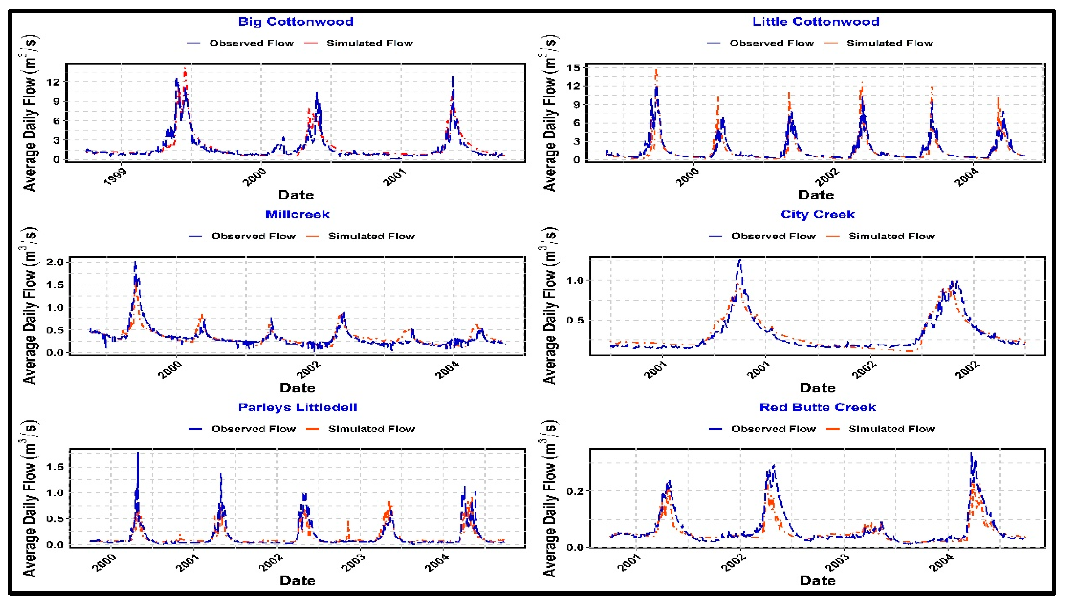
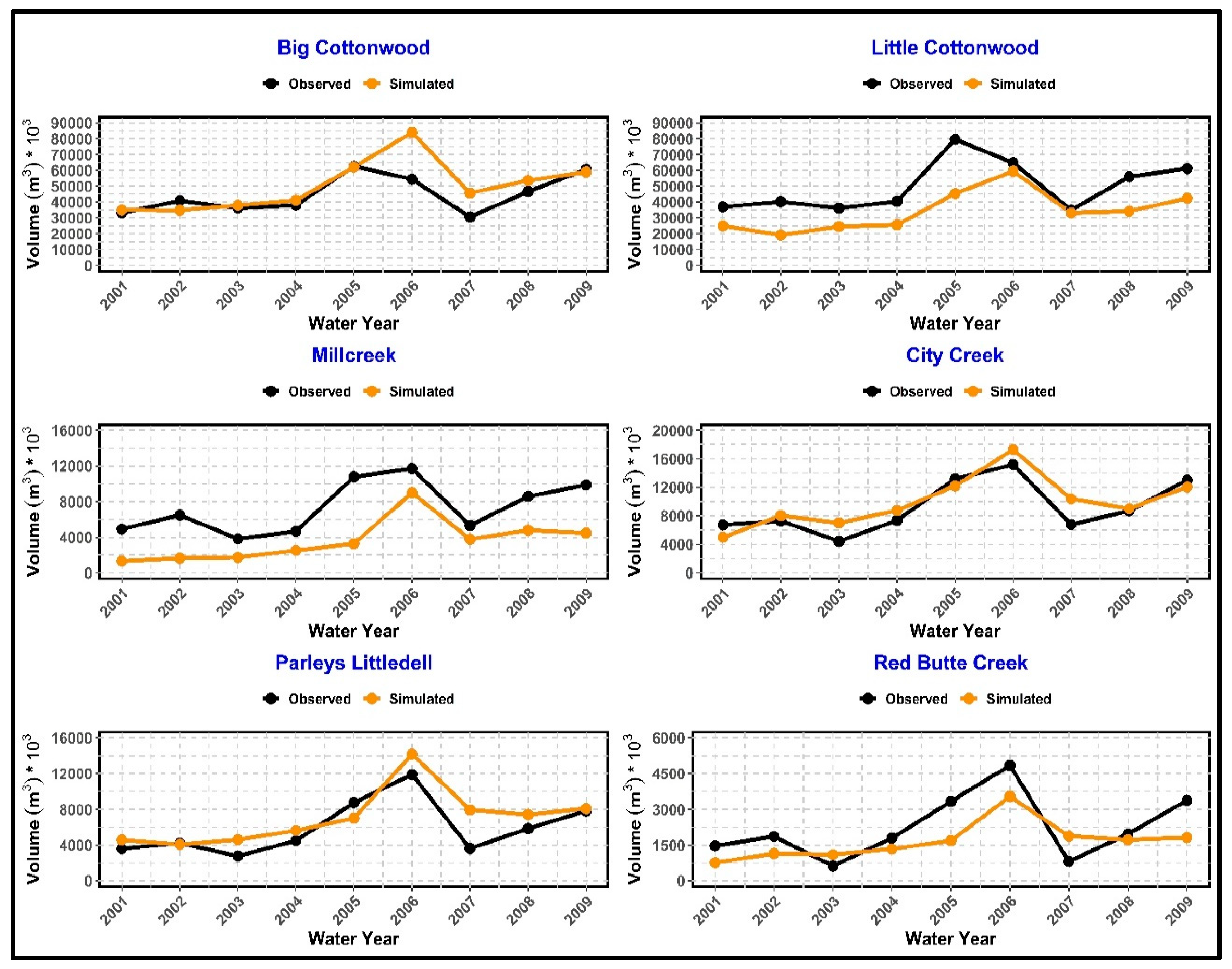
The observed and simulated hydrographs for the calibration period of the hydrologic models of six watersheds are shown in
Figure 5. Overall, the model slightly underestimated the peak flows for all the watersheds except Little Cottonwood and estimated reasonably well the dry season base flow in most of the cases.
Results of the statistical tests performed to evaluate the models’ performance are shown in
Table 3. The Nash–Sutcliffe efficiency indices of the models were within the range of 0.71 to 0.83 with the lowest (0.71 for Parleys Littledell) indicating a very good to satisfactory fit of simulated and observed streamflow in terms of amount and timing of flows. Similarly, the coefficient of determination (R
2) for the models ranges from 0.721 to 0.841, which means the performance rating of developed calibrated hydrologic models for four out of six watersheds were very good while the performance ratings of Little Cottonwood and Red Butte Creek models were good. A percent error volume (PEV) test was also done to understand the models’ performance in terms of estimating the total volume of water for the whole calibration period. From the PEV tests, it was clear that the performance of all the hydrologic models was very good except for Little Cottonwood and Red Butte Creek. The performances of those two models were good. Model results were evaluated using those statistical tests according to general performance ratings for recommended statistics (
Table 4) [
52].
Calibration results indicate that the developed models were unable to reliably generate flows under specific climatic circumstances like when the streams became frozen and flows due to heavy snow and rain occurred on the same day. The models also struggled to predict small peaks due to small, isolated rainfall events in summer. From the PEV results, it was found that the models for Little Cottonwood, Red Butte Creek, and Parleys Littledell underestimated the total volume of water, whereas the models for Big Cottonwood, Millcreek, and City Creek overestimated the total volume of water over the calibration period.
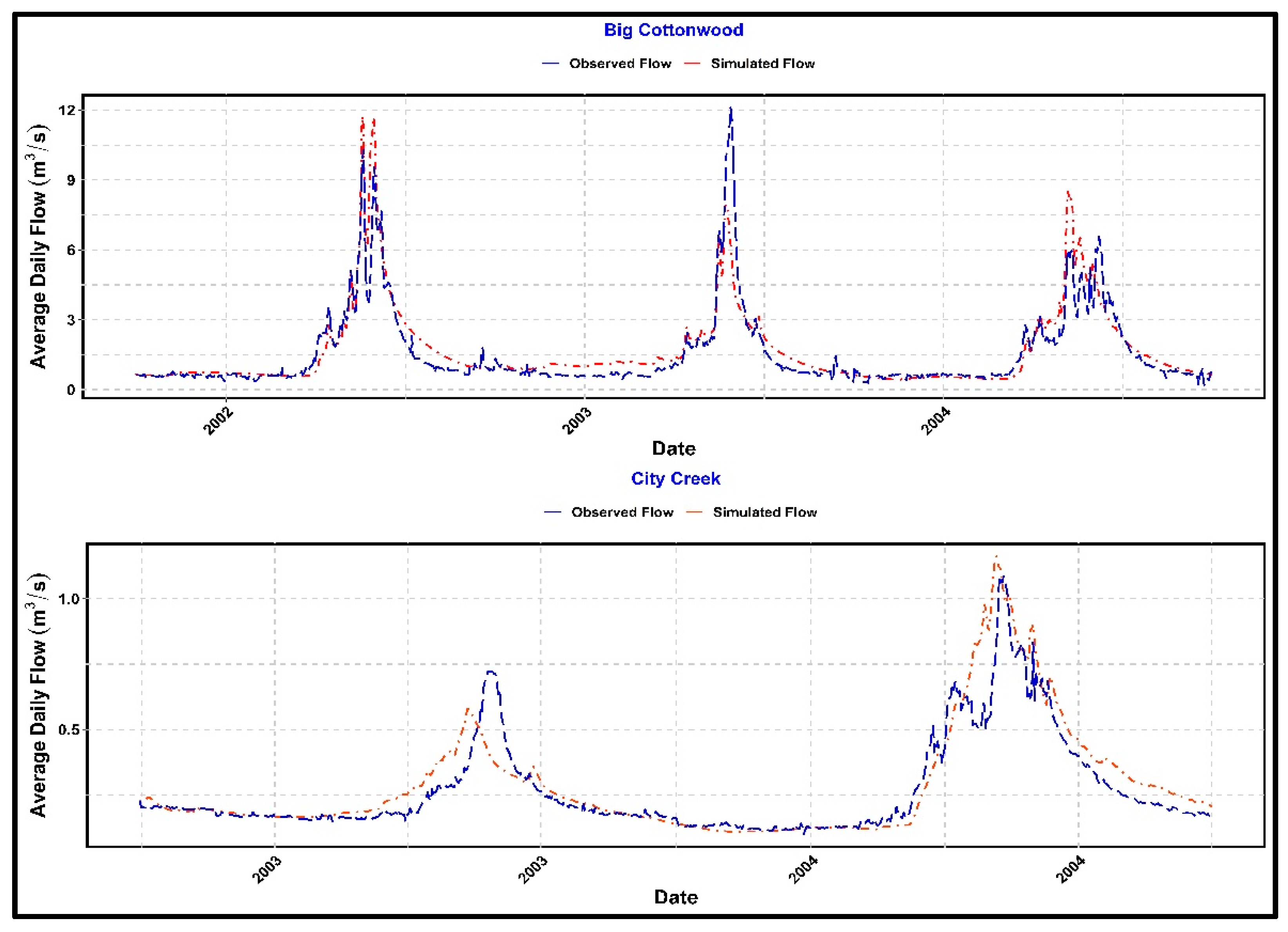
Figure 6 shows the validation results of Big Cottonwood and City Creek. The statistical analyses for the validation run shown in
Table 5 do not exhibit any significant difference with the calibration results. The downside of calibrating for shorter periods is that there is greater potential to miss the range of hydrologic variability so the four remaining watersheds used a longer calibration period.
3.2. Historical Baseline Scenario
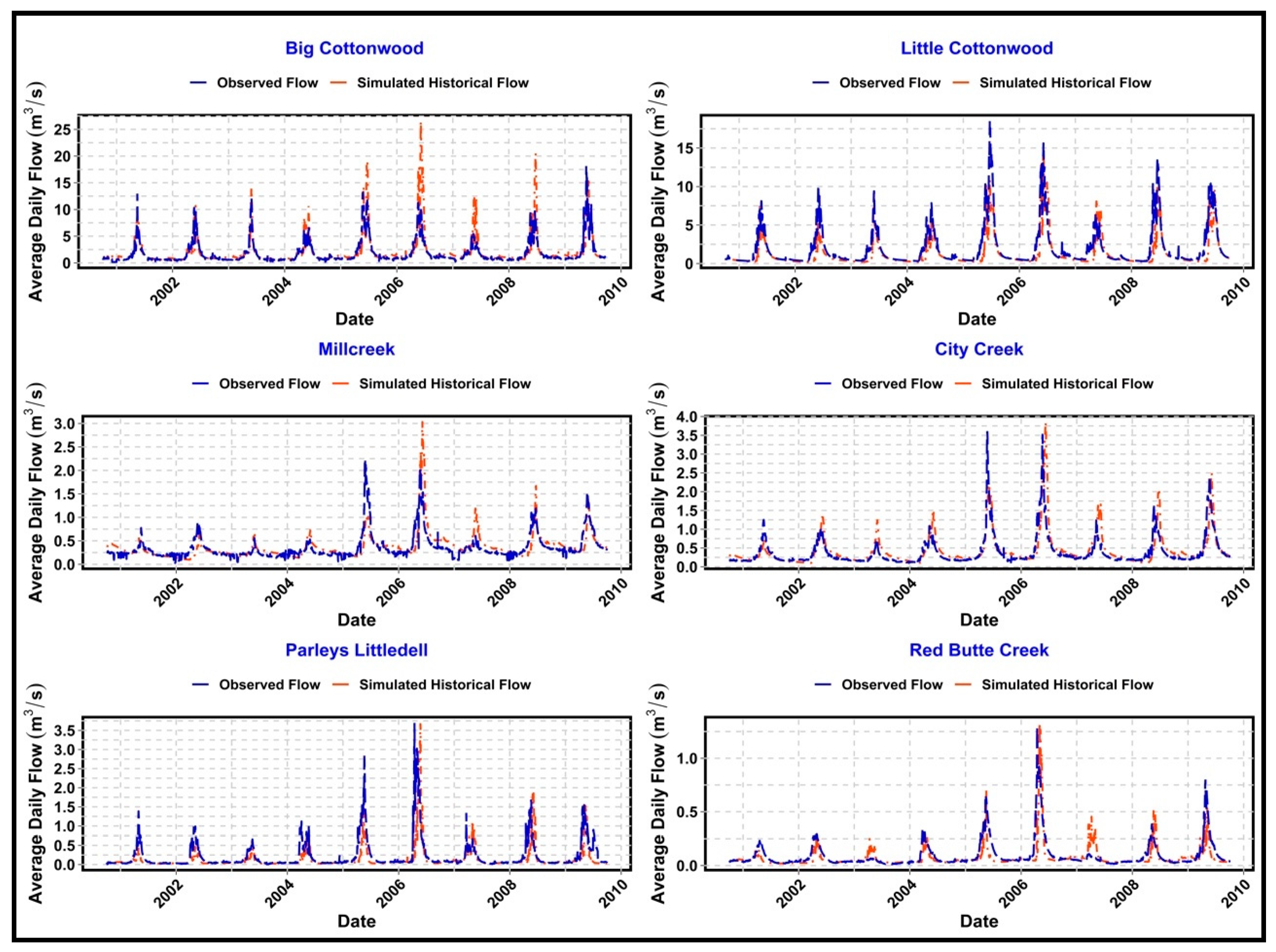
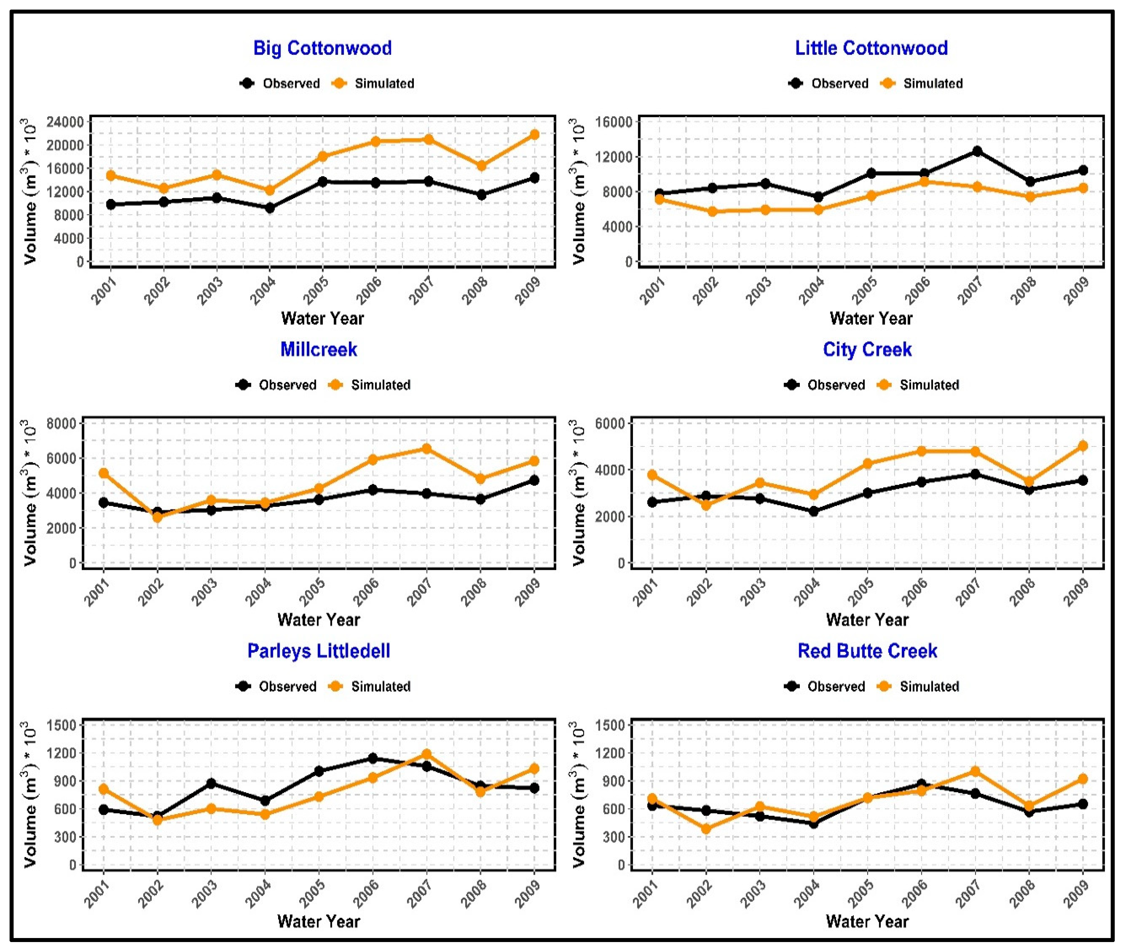
The observed and simulated hydrographs of six watersheds for the historical baseline period are shown in
Figure 7. Unlike the calibration period, the model slightly overestimated the peak flows for all the watersheds except for Little Cottonwood and Parleys Littledell and estimated reasonably well the dry season base flow in most of the cases. Although the timing of the simulated peak runoffs were usually delayed compared to the observed peak flows, the base flows during the historical baselines were estimated satisfactorily by the model, which is important for estimating drought impacts on water supply and ecosystem services.
The NSE values comparing observed and simulated stream runoff ranged from 0.41 to 0.72 (
Table 6) for the six models. In terms of NSE and R
2 values, Little Cottonwood and City Creek watersheds exhibited good and satisfactory fits with the observed flow, respectively. The coefficients of determination ranged from 0.52 to 0.77, with values above 0.50 indicating an acceptable fit between observed and simulated flows (
Table 6) for all the watersheds. The NSE and R
2 analysis suggests that the model can predict the amount of flow at a satisfactory level for all the watersheds but might not be able to predict the timing of the flow at a satisfactory level for all the watersheds except Little Cottonwood and City Creek.
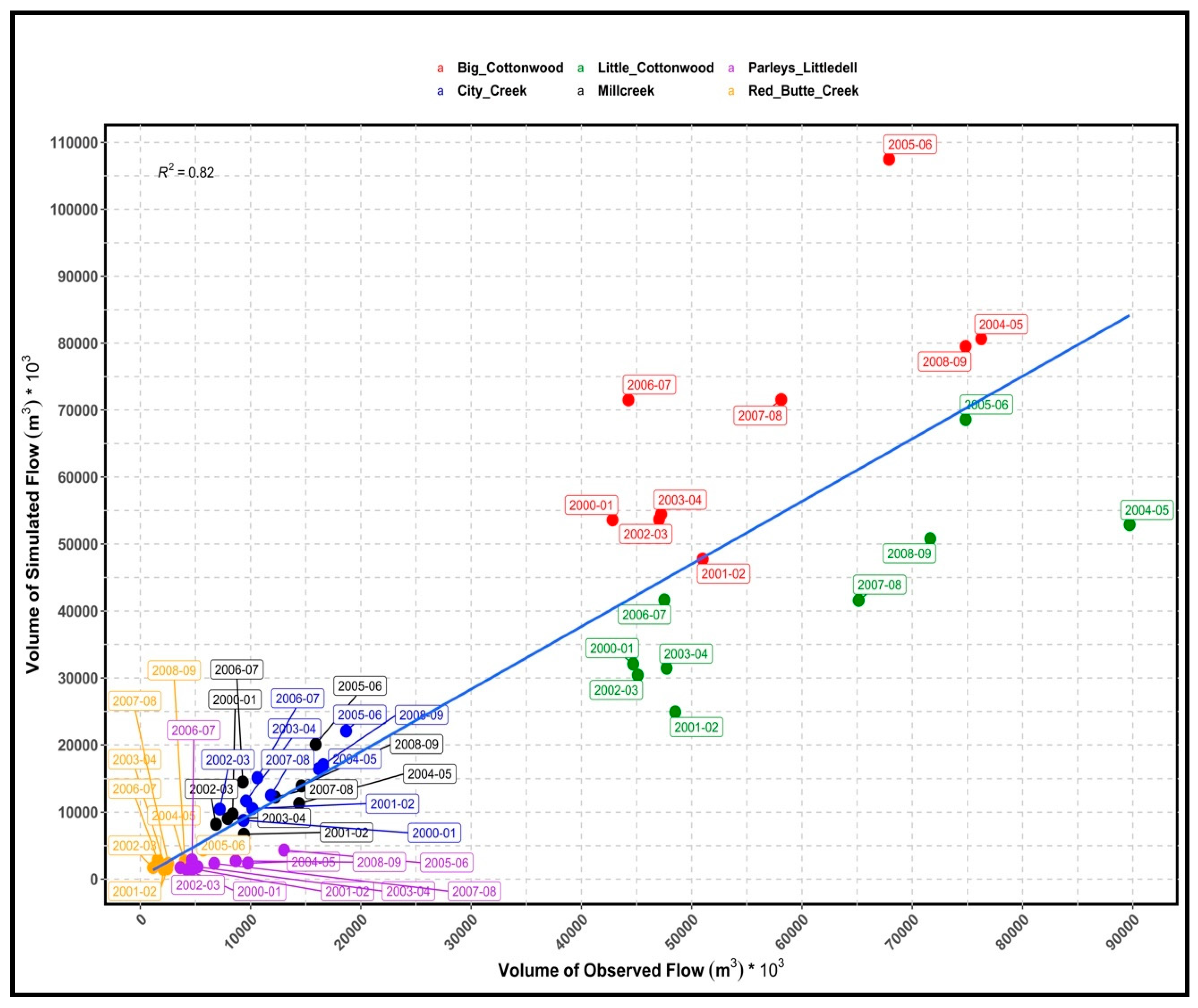
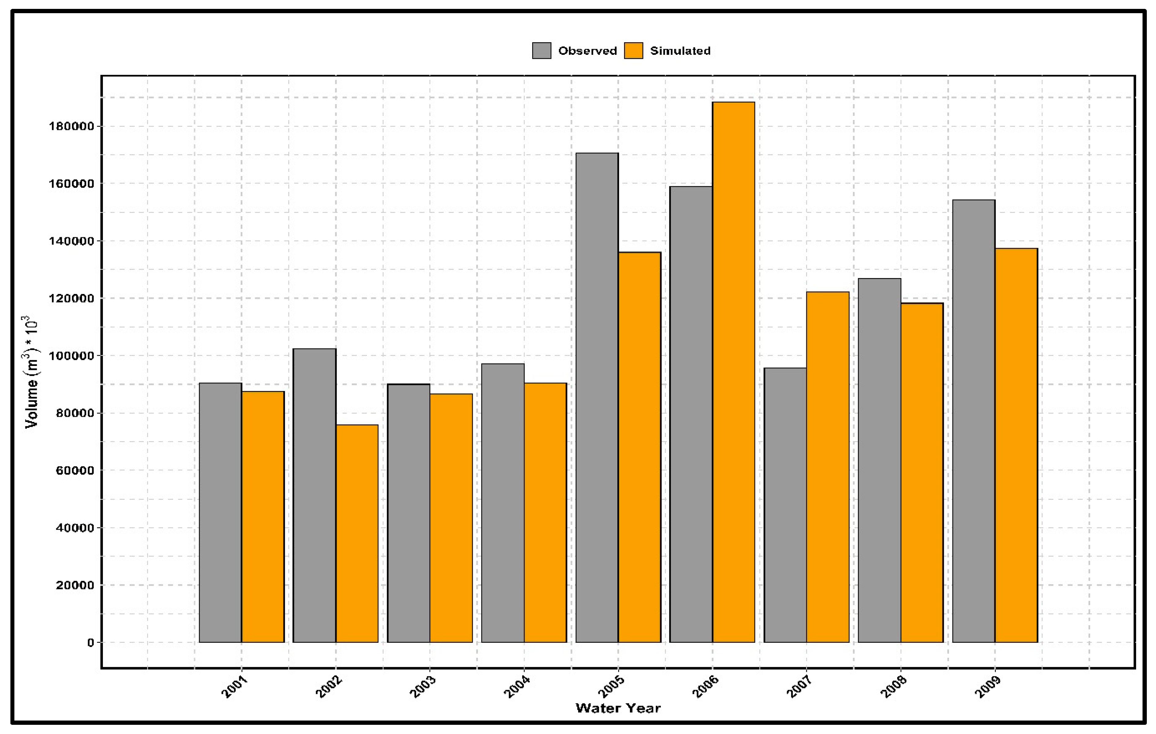
Simulation of flows (peak and base) is conventional for the acceptance of the validity of a model, but for water supply and drought analysis, the available volume is more important and relevant. Moreover, as we wanted to evaluate the performance of the dynamically downscaled climate fields by using them to force a hydrologic model, we also tried to analyze the results of the historical baseline simulation in terms of the total annual volume of flow and seasonal volume of flow. The water year in the USA starts on 1 October and ends on 30 September. For our analysis, we considered March through August of a water year as the peak seasonal flow period and October through February plus September as the dry season flow period. The total annual volume of water analysis (
Figure 8) showed that simulated volumes of water were higher than the observed total annual volume of water for Big Cottonwood, City Creek, and Millcreek and lower than the observed volumes of water for Little Cottonwood, Red Butte Creek, and Parleys Littledell. These results were similar to observations found in the calibration results, although the bias in the volume of water was higher. The value of R
2 is 0.82, which shows a very good fit between the simulated and the observed annual volume of water taking all the watershed into consideration.
While
Figure 8 gives an overall indication of the performance of the historical climate projections based on the simulated and the observed annual volume of water, the statistical analysis shown in
Table 7 provides a better representation of the performance of dynamically downscaled climate projections for the individual watersheds. The R
2 value of 0.82 and 0.70 show a very good and good fit for City Creek and Parleys Littledell respectively while indicating a satisfactory fit for all the other watersheds. PEV analysis shows a very good fit for Millcreek and good to satisfactory fit for all the other watersheds except Big Cottonwood.
Peak seasonal volume analysis (
Figure 9) shows that except for Little Cottonwood and Millcreek watersheds, the simulated volume of peak seasonal flow matched reasonably well with the observed volume for other watersheds (the differences in the smaller watersheds are due to scale). The simulated volume of peak seasonal flow for Little Cottonwood and Millcreek is lower than the volume of observed flow throughout the historical baseline period. In the case of dry season volume analysis (
Figure 10), the model matched well with the observed volumes for the smaller watersheds but overestimated for Big Cottonwood, Millcreek, and City Creek while slightly underestimating the volumes for Little Cottonwood and Parleys Littledell watersheds.
Results of the statistical tests performed to evaluate the models’ performance in terms of seasonal flow volume analysis are shown in
Table 8. Considering the R
2 value, the model simulations of peak and dry season volume varied from satisfactory to very good for all the watersheds. In terms of the PEV analysis, the model simulations are inconclusive although the performance ratings are slightly better for dry season volumes compared to peak seasons’ considering two very good ratings for dry season compared to one for peak season, and the average error is slightly lower in dry season (21% as against about 24%) compared to peak season. From the seasonal volume flow analysis perspective, it can be concluded that the models performed better in estimating dry season flow (considering better R
2 values and slightly higher PEV ratings) than the peak season flow. High spatial variability in winter storms (discussed later in the uncertainties section) is a likely cause for peak flow discrepancies. From the seasonal volume analysis perspective, it can be concluded that the models performed better in estimating dry season flow (considering better R
2 values and slightly higher PEV ratings) than the peak season flow. High spatial variability in winter storms (discussed later in the uncertainties section) is a likely cause for peak flow discrepancies.
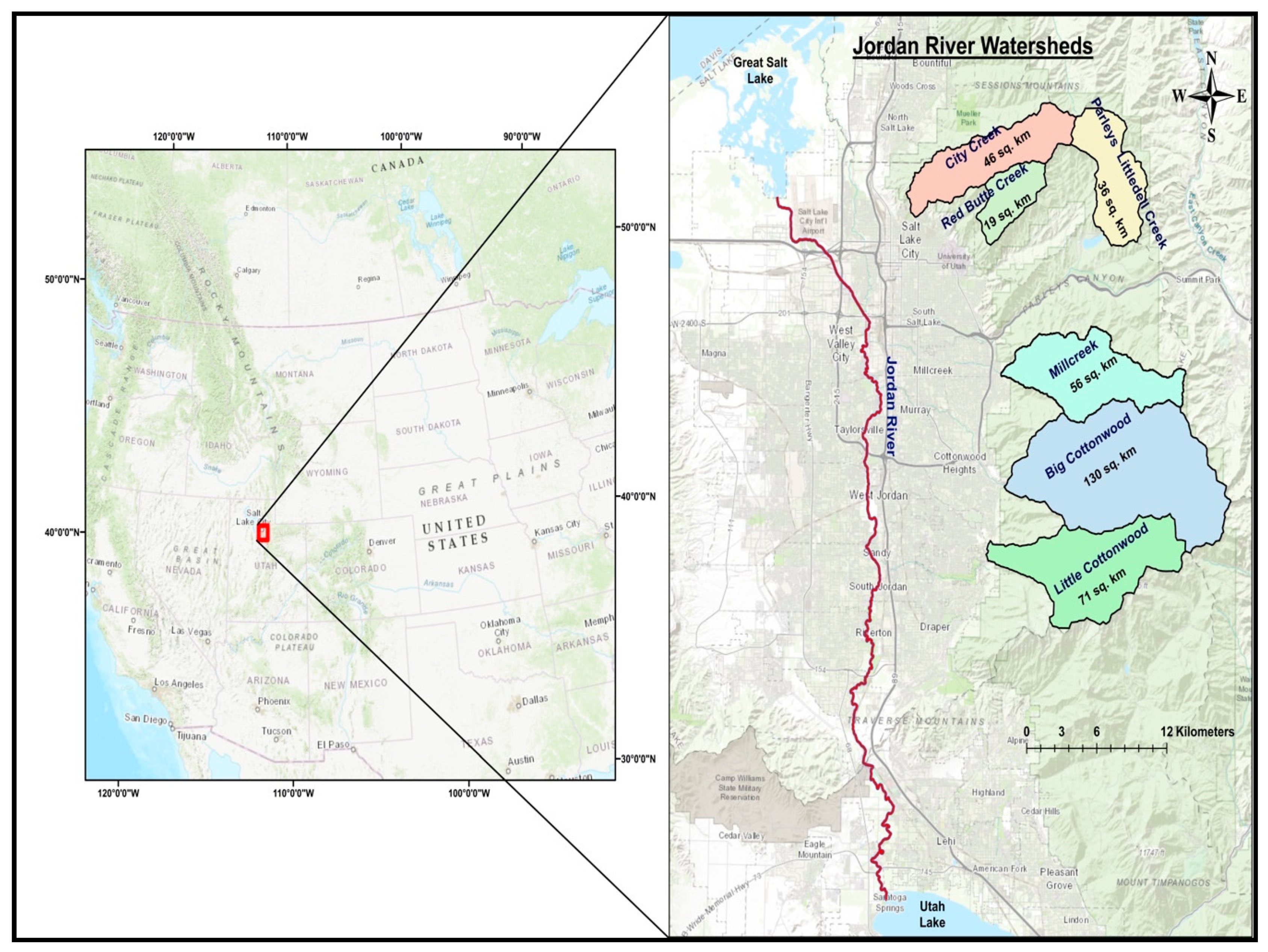
These six watersheds are the major contributors to the Jordan River downstream of Utah Lake and are the primary sources of drinking water for Salt Lake City, so to get a better understanding of how the dynamically downscaled climate projection depicts the downstream drinking water supply, we compared the total volume of simulated flow coming from theses six watersheds to the observed total volume. As presented in
Figure 11, the total amount of simulated flow is comparable but slightly lower than the observed flow for all the years except WY 2005–2006 and 2006–2007. Over the 9-year period for the Jordan River basin, the total amount of simulated flow is 4% lower than the total amount of observed flow.
In mountainous watersheds, the form of precipitation and snow melting processes depend strongly on elevation as snowfall increases rapidly with elevation and the melting of snow at the beginning of the season starts at lower elevations [
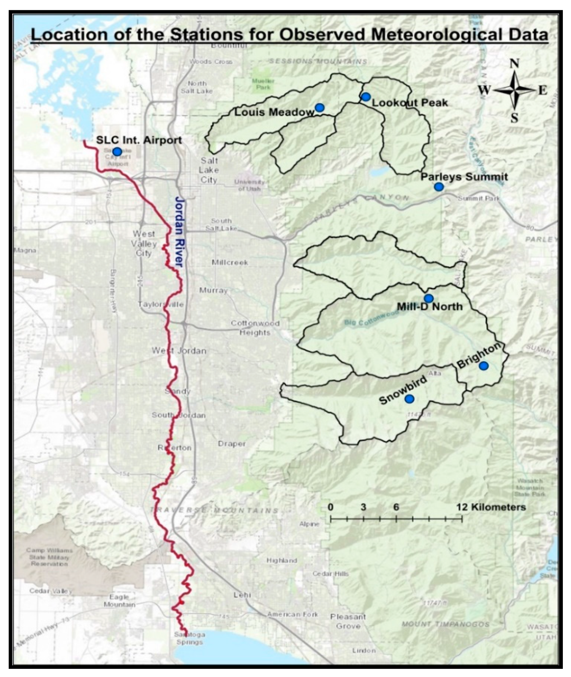
57]. The observed data from the SNOTEL stations did not provide a clear indication about the transformation of a precipitation event from snow to rain or vice versa with the change in elevation. Additional snow stations would help to get a better estimation of the spatial variability of the snow depth.
Although the six watersheds are located adjacent to each other, they are very unique in terms of elevation, slope, aspect, soil types, and vegetation. DHSVM is a physically distributed model so elevation, aspect, and slope were handled quite well. In the case of soil parameters, however, the basin models were predominantly based on values obtained from previous studies and default model values since no watershed-specific measurements of soil depth, hydraulic properties, and soil moisture parameters were found in the literature. The lack of site-specific parameter data likely increases the uncertainty in model results. Soil types vary from bedrock to sandy loam to clay loam or granular silt loam among neighboring watersheds. Furthermore, sometimes the same soil in different watersheds might have different soil properties due to the geographical and overall condition of the watershed. Vegetation parameters like height, root zone depth, and leaf area index (LAI) were derived from the readily available literature and various online databases. The use of generalized values of the input parameters due to lack of region-based observed or measured values could have contributed to lower the model efficiency.
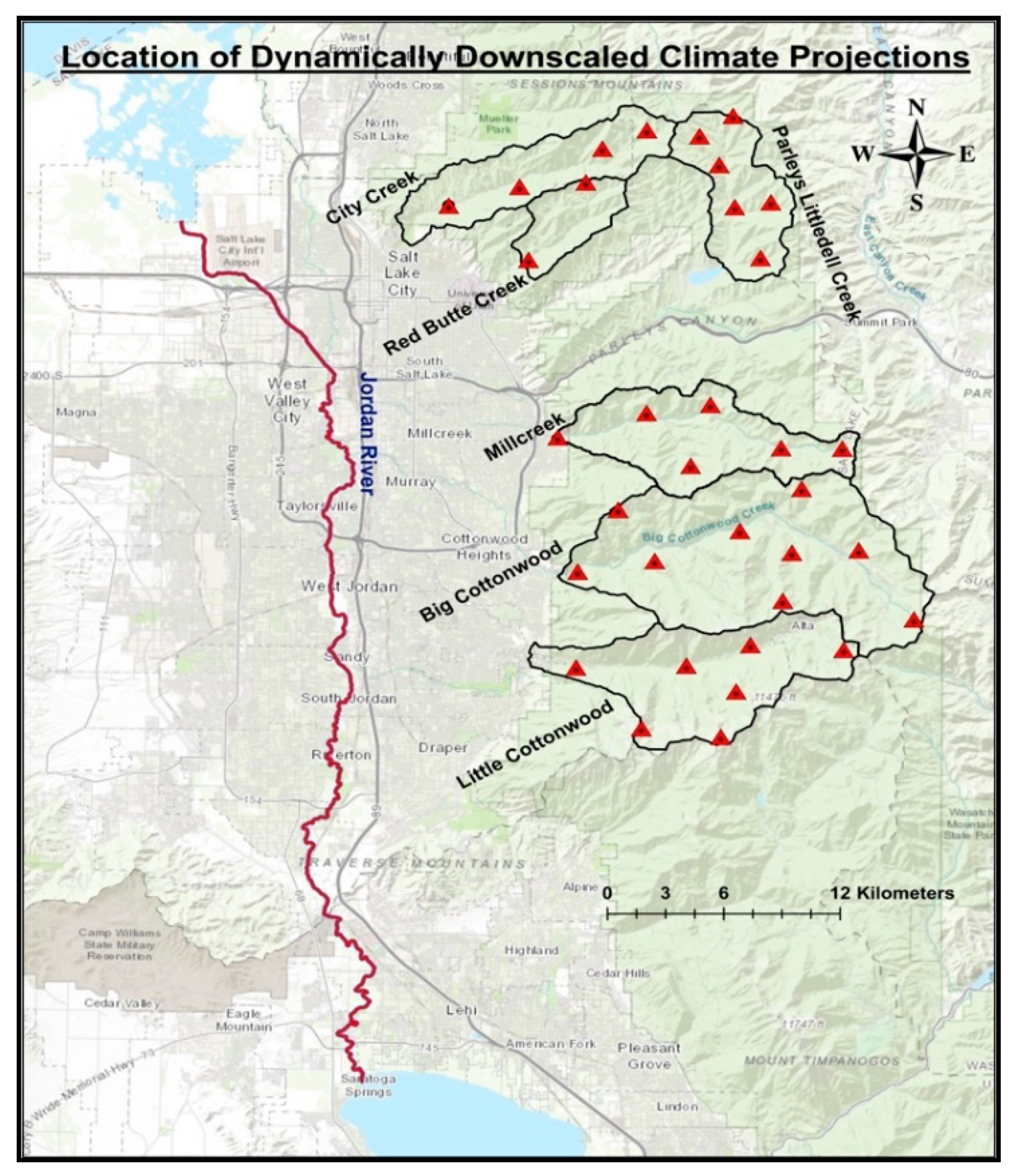
The spatial scale of DHSVM is 30 m, whereas the spatial resolution of the dynamically downscaled climate projection is 4 km. Although fine-scale downscaling of climate predictions from 4 km to 90 m has been done in some areas for temperature and precipitation [
58], the process characteristics and data sets required to reduce downscaling uncertainties in most mountainous watersheds, including those in our study area, does not typically exist, specifically for the parameters we used in this study. Moreover, the study [
58] shows no significant difference in precipitation amount between the 4 km grid and the 90 m grid. Also, dynamic downscaling below 4-km in complex terrain with sparse observations does not increase skill in the representation of meteorological fields [
59], and attempting to downscale below 4-km resolution for the length of study we have here would be computationally prohibitive. It is also important to mention that all downscaling techniques have their inherent biases and percentage of error, which might even introduce further uncertainties in the output. As detailed in Scalzitti et al. [
27], the data we used have undergone extensive validation, and the previous study [
58] showed there is no significant difference in precipitation and temperature by further spatial downscaling from 4 km to a smaller grid, so we used the dynamically downscaled climate projection directly to the 30 m grid of DHSVM. Therefore, the results presented in this study may have some uncertainty related to scale interaction, which can be addressed with improved higher resolution spatial scale climate projection in future research.
