Perturbation Solution for Pulsatile Flow of a Non-Newtonian Fluid in a Rock Fracture: A Logarithmic Model

Abstract

The purpose of this work is to study the motion of a non-Newtonian fluid in a rock fracture, generated by a constant pressure gradient to which a pulsating component is superposed. The momentum equation is faced analytically by adopting a logarithmic constitutive law; the velocity is expressed as a power series of the amplitude of the pulsating component, up to the second order, easily usable for numerical calculations. The results obtained are compared with those provided in the past by the authors, using a three-parameter Williamson model. The comparison highlights that the value of the mean flow rate in a period differs by less than 10% even if the velocity profiles look quite different.

1. Introduction

It is well known that the fluid flow within a geological formation takes place mainly through fractures that are often connected to each other to constitute a network. The study of motion through fractures affects many industrial activities, such as exploitation of a basin, oil and gas extraction, contaminant pollution control and hydraulic fracturing. In enhanced oil recovery operations, polymer solutions that exhibit a non-Newtonian shear-thinning behavior are injected [1].

A literature overview shows that when an oilfield is flooded with a non-Newtonian fluid, the mobility ratio between the displaced fluid and the displacing fluid becomes favorable with respect to flooding with water. Oil displacement tests indicate that water-soluble polymer added to the injection water can recover additional oil from an oilfield. The polymers often used are polyacrylamide or polysaccharide; these substances provide the highest viscosity for an assigned concentration.

The description of the flow in a single fracture has been addressed both analytically and experimentally. With an analytical approach to the problem, and schematizing the rheological behavior of the fluid with a Newtonian one, the cubic law expresses the hydraulic transmissivity as a function of the average fracture opening, assuming that the rough walls can be schematized with two smooth parallel plates [2]. However, the roughness of natural rock fractures, the variability of the aperture, and the presence of obstructions, complicate the process that deviates from a Poiseuille flow; in [3], the flow tortuosity and the aperture variation are considered to modify the cubic law to simulate numerically the flow. The experimental work [4] investigates the influence of geometric characteristics of deformable rough fractures, and the relationships between the hydraulic gradient and the flow rate. Despite the importance of the effects of roughness in fracture flow—as emphasized in the reference work of Zimmerman and Bodvarsson [5]—the roughness is neglected in the present paper because, for an analytical analysis, the complexity generated by the rheological constitutive law of a non-Newtonian fluid and by the unsteady flow suggests adopting a simplified geometry to solve the problem.

Tsang [6] and Neuzil [7] show that the scheme of plane motion gives reliable results if the normal stress is less than ~10 MPa, and if the aperture variation along the flow path is not large.

The plane unsteady flow of a non-Newtonian fluid has been faced by many authors even recently, either for numerical calculation purposes or analytically. Particularly, the motion generated superposing to a constant pressure gradient a small periodical variation has acquired technical and practical uses, because it allows the growth of the mean discharge with a limited increase of power. The non-linearity of the constitutive equation of pseudoplastic fluids makes the variation of the rate of flow during the phase of increase of the pressure gradient exceed the decrease occurring when it falls.

In this paper, the forcing action is given by a constant pressure gradient and a small periodic variation superposed to it.

In the first part, the phenomenon is studied, adopting a constitutive equation given by a logarithmic law (L), which can be considered as a simplified Prandl–Eyring model, and represents, with good approximation, the behavior of pseudoplastic materials (particularly of polymer solution and powder suspensions in Newtonian fluids), in a wide range of shear stress and shear rate. The results will be compared to those obtained by the authors using a Williamson model (W), proposed in [8] for the same fluid and the same geometry [9].

The momentum equation is solved using a perturbation method, assuming the amplitude of the pulsatile component of the pressure gradient as a parameter. It is a method widely used to obtain approximated solutions to engineering problems, even if the convergence of the solution is not normally demonstrable.

In particular, the second-order term of the velocity field that gives origin to a variation of the mean discharge will be determined; it will always result positive, thus justifying analytically the intuitive fact that the mean flow rate in a period increases.

2. Problem statement

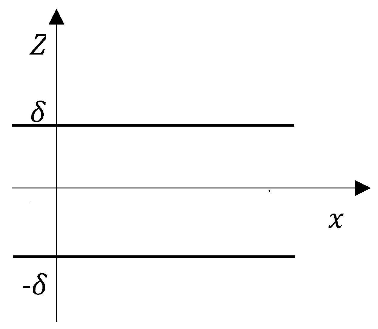
The plane laminar flow of an incompressible non-Newtonian fluid, in a layer of thickness $2\delta$, as shown in Figure 1, is considered, under the action of a small periodic pressure gradient superimposed on a constant one. A sensitivity analysis to test the influence of the roughness would require solving the problem numerically and making a comparison of the results. However, this goes beyond the purpose of this paper, which aims to compare the results provided by using the same fluid with two different models to approximate the experimental points representing the relationship between shear-stress and shear-rate.

Figure 1. Schematic representation of the geometry.

The velocity is supposed to have the $x$ direction; taking into account the continuity equation, the equation of motion can be written as

$$-\frac{\partial p}{\partial x}+\frac{\partial \overline{\tau }}{\partial Z}=\rho \frac{\partial u}{\partial T}$$

(1)

where $Z$ is normal to the layer, $T$ is the time, $p$ the pressure, ρ the fluid density, $\overline{\tau }$ the shear stress and $u$ the velocity.

The fluid considered is a pseudoplastic one, and a simple two-parameter model based on a logarithmic law, which is similar to the Prandtl–Eyring model $\overline{\tau }={\overline{\tau }}_0{\sinh }^{-1}\left(\lambda \dot{\gamma }\right)$, can be used:

$$\overline{\tau }={\overline{\tau }}_0\ln \left(1+\lambda \left|\dot{\gamma }\right|\right)\mathrm{sign}\left(\dot{\gamma }\right)$$

(2)

where $\dot{\gamma }$ is the shear rate $\partial u/\partial Z$, and ${\overline{\tau }}_0$ and $\lambda$ are two rheological parameters.

The flow is symmetric with respect to the $x$ axis, and thus the problem is studied only in the region $-\delta \le Z\le 0$ where $\dot{\gamma }\ge 0$, and thus

$$\overline{\tau }={\overline{\tau }}_0\ln \left(1+\lambda \dot{\gamma }\right)$$

(3)

The imposed pressure gradient is

$$-\frac{\partial p}{\partial x}=P_0\left(1+\epsilon \cos \omega T\right)$$

(4)

$P_0$ is the constant pressure gradient, $\epsilon$ is the amplitude of the periodic perturbation and $\omega$ its pulsation. Equation (1) becomes

$$P_0\left(1+\epsilon \cos \omega T\right)+\frac{\partial \overline{\tau }}{\partial Z}=\rho \frac{\partial u}{\partial T}$$

(5)

Introducing the following dimensionless quantities $z=Z/\delta$, $t=T/\lambda$, $\mathsf{\Omega }=\omega \lambda$, $v=u\lambda /\delta$, $\tau =\overline{\tau }{\lambda }^2/\left(\rho {\delta }^2\right)$, $\mu ={\overline{\tau }}_0{\lambda }^2/\left(\rho {\delta }^2\right)$, $p_0=P_0{\lambda }^2/\left(\rho \delta \right)$, Equation (5) becomes

$$p_0\left(1+\epsilon \cos \mathsf{\Omega }t\right)+\mu \frac{\partial }{\partial z}\left[\ln \left(1+\frac{\partial v}{\partial z}\right)\right]=\frac{\partial v}{\partial t}$$

(6)

Supposing $\epsilon \ll 1$, the velocity is expanded as a power series in $\epsilon$

$$v\left(z,t\right)=v_0\left(z\right)+\epsilon v_1\left(z,t\right)+{\epsilon }^2{v}_2\left(z,t\right)+O\left({\epsilon }^3\right)$$

(7)

and thus

$$1+\frac{\partial v}{\partial z}=1+\frac{d{v}_0}{dz}+\epsilon \frac{\partial v_1}{\partial z}+{\epsilon }^2\frac{\partial v_2}{\partial z}+O\left({\epsilon }^3\right)$$

(8)

Putting

$$w_0=1+\frac{d{v}_0}{dz}$$

(9)

Equation (8) becomes

$$1+\frac{\partial v}{\partial z}=w_0\left[1+\frac{\epsilon }{w_0}\frac{\partial v_1}{\partial z}+\frac{{\epsilon }^2}{w_0}\frac{\partial v_2}{\partial z}+O\left({\epsilon }^3\right)\right]$$

(10)

Taking the logarithm of the two terms and developing the second member in power series, we obtain:

$$\ln \left(1+\frac{\partial v}{\partial z}\right)=\ln w_0+\frac{\epsilon }{w_0}\frac{\partial v_1}{\partial z}+\frac{{\epsilon }^2}{w_0}\frac{\partial v_2}{\partial z}-\frac{{\epsilon }^2}{2w_0^2}{\left(\frac{\partial v_1}{\partial z}\right)}^2+O\left({\epsilon }^3\right)$$

(11)

Substituting Equation (11) in (6)

$$p_0\left(1+\epsilon \cos \mathsf{\Omega }\mathrm{t}\right)+\mu \frac{\partial }{\partial z}\left\{\ln w_0+\frac{\epsilon }{w_0}\frac{\partial v_1}{\partial z}+\frac{{\epsilon }^2}{w_0}\left[\frac{\partial v_2}{\partial z}-\frac{1}{2w_0}{\left(\frac{\partial v_1}{\partial z}\right)}^2\right]\right\}=\epsilon \frac{\partial v_1}{\partial t}+{\epsilon }^2\frac{\partial v_2}{\partial t}$$

(12)

Equating the coefficients of the same order in $\epsilon$, three equations follow:

$$p_0+\mu \frac{d}{dz}\ln \left(1+\frac{d{v}_0}{dz}\right)=0$$

(13)

$$p_0\cos \mathsf{\Omega }\mathrm{t}+\mu \frac{\partial }{\partial z}\left(\frac{1}{w_0}\frac{\partial v_1}{\partial z}\right)=\frac{\partial v_1}{\partial t}$$

(14)

$$\mu \frac{\partial }{\partial z}\left[\frac{1}{w_0}\frac{\partial v_2}{\partial z}-\frac{1}{2w_0^2}{\left(\frac{\partial v_1}{\partial z}\right)}^2\right]=\frac{\partial v_2}{\partial t}$$

(15)

The velocity $v_0$,$v_1$ and $v_2$ must satisfy the boundary conditions $v_k\left(-1\right)=0$ and ${\frac{\partial v_k}{\partial z}|}_{z=0}=0$, where $k=0, 1, 2$.

2.1. The Steady Component

Equation (13) has the solution

$$v_0\left(z\right)=-\frac{\exp \left(-\alpha z\right)}{\alpha }-z+C$$

(16)

where $\alpha =p_0/\mu$. It must be $v_0\left(-1\right)=0$ and thus $C=\frac{\exp \left(\alpha \right)}{\alpha }-1$ and

$$v_0\left(z\right)=\frac{\exp \left(\alpha \right)-\exp \left(-\alpha z\right)}{\alpha }-\left(1+z\right)$$

(17)

which gives a steady rate of flow

$$Q_0=2\underset{-1}{\overset{0}{{\displaystyle \int }}}{v}_0\left(z\right)dz=2\left(\frac{1+\left(\alpha -1\right)\exp \left(\alpha \right)}{{\alpha }^2}-\frac{1}{2}\right)$$

(18)

2.2. The First-Order Approximation

Writing the solution of Equation (14) in the form

$$v_1\left(z,t\right)=\mathrm{Re}\left[w_1\left(z\right)\exp \left(i\mathsf{\Omega }\mathrm{t}\right)\right]$$

(19)

Equation (14) becomes

$$p_0+\mu \frac{d}{dz}\left(\frac{1}{w_0}\frac{d{w}_1}{dz}\right)=i\mathsf{\Omega }{w}_1$$

(20)

which has the particular integral $w_{10}=-i\frac{p_0}{\mathsf{\Omega }}$; the solution of Equation (20) can be written as $w_1=w_{10}+W_1$, where $W_1$ is the solution of the homogeneous equation

$$\mu \frac{d}{dz}\left(\frac{1}{w_0}\frac{d{W}_1}{dz}\right)-i\mathsf{\Omega }{W}_1=0$$

(21)

Putting $\xi =k\exp \left(-\alpha z/2\right)$, where $k=2\sqrt{\mu \mathsf{\Omega }}/p_0$ and recalling that

$$w_0=1+\frac{\partial v_0}{\partial z}=\exp \left(-\alpha z\right)={\xi }^2\frac{p_0^2}{4\mathsf{\Omega }\mu }$$

(22)

Equation (21) can be recast in the form

$$\xi \frac{d^2{W}_1}{d{\xi }^2}-\frac{d{W}_1}{d\xi }-i\xi W_1=0$$

(23)

which admits the solution [10]

$$W_1\left(\xi \right)=\xi \left\{A\left[{\mathrm{ber}}_1\left(\xi \right)+i{\mathrm{bei}}_1\left(\xi \right)\right]+B\left[{\ker }_1\left(\xi \right)+i{\mathrm{kei}}_1\left(\xi \right)\right]\right\}$$

(24)

where ${\mathrm{ber}}_1$, ${\mathrm{bei}}_1$, ${\ker }_1$ and ${\mathrm{kei}}_1$ are the well-known Kelvin function of order 1, $A=a_1+i{a}_2$ and $B=b_1+i{b}_2$ are suitable constants to be calculated, imposing the boundary conditions $v_1\left(z=-1\right)=v_1\left[\xi =k\exp \left(\alpha /2\right)\right]=0$ and ${\frac{\partial v_1}{\partial z}|}_{z=0}=-\frac{\alpha \xi }{2}{\frac{\partial v_1}{\partial \xi }|}_{\xi =k}=0$, i.e., ${\frac{\partial v_1}{\partial \xi }|}_{\xi =k}=0$. The solution of Equation (20) is thus

$$w_1\left(\xi \right)=w_{10}+W_1\left(\xi \right)=-i\frac{p_0}{\mathsf{\Omega }}+\xi \left[U_1\left(\xi \right)+i{U}_2\left(\xi \right)\right]$$

(25)

where

$$U_1\left(\xi \right)=a_1{\mathrm{ber}}_1\left(\xi \right)-a_2{\mathrm{bei}}_1\left(\xi \right)+b_1{\ker }_1\left(\xi \right)-b_2{\mathrm{kei}}_1\left(\xi \right)$$

(26)

and

$$U_2\left(\xi \right)=a_1{\mathrm{bei}}_1\left(\xi \right)+a_2{\mathrm{ber}}_1\left(\xi \right)+b_1{\mathrm{kei}}_1\left(\xi \right)+b_2{\ker }_1\left(\xi \right)$$

(27)

The solution of the first-order approximation becomes

$$v_1\left(\xi ,t\right)=\mathrm{Re}\left[w_1\left(\xi \right)\exp \left(i\mathsf{\Omega }\mathrm{t}\right)\right]=\xi U_1\left(\xi \right)\cos \mathsf{\Omega }t+\left[\frac{p_0}{\mathsf{\Omega }}-\xi U_2\left(\xi \right)\right]\sin \mathsf{\Omega }t$$

(28)

2.3. Second-Order Approximation

Equation (15) contains the term

$${\left(\frac{\partial v_1}{\partial z}\right)}^2={\left\{\frac{\partial }{\partial z}\mathrm{Re}\left[w_1\left(z\right)\exp \left(i\mathsf{\Omega }\mathrm{t}\right)\right]\right\}}^2={\left\{\mathrm{Re}\left[\frac{d{w}_1}{dz}\exp \left(i\Omega t\right)\right]\right\}}^2$$

(29)

Recalling that for every complex number $\zeta$ it results ${\left[\mathrm{Re}\left(\zeta \right)\right]}^2=\frac{1}{2}\left[\mathrm{Re}\left({\zeta }^2\right)+{\left|\zeta \right|}^2\right]$, and observing that $\frac{d{w}_1}{dz}=\frac{d{W}_1}{dz}$, Equation (29) gives

$${\left(\frac{\partial v_1}{\partial z}\right)}^2=\frac{1}{2}\left\{\mathrm{Re}\left[{\left(\frac{d{W}_1}{dz}\right)}^2\exp \left(2i\Omega t\right)\right]+{\left|\frac{d{W}_1}{dz}\right|}^2\right\}$$

(30)

Searching a solution of Equation (30) in the form

$$v_2\left(z,t\right)=v_{20}\left(z\right)+\mathrm{Re}\left[w_2\left(z\right)\exp \left(2i\mathsf{\Omega }\mathrm{t}\right)\right]$$

(31)

allows to write Equation (15) as follows

$$\begin{array}{l}\mu \frac{d}{dz}\left\{\frac{1}{w_0}\frac{d{v}_{20}}{dz}+\frac{1}{w_0}\mathrm{Re}\left[\frac{d{w}_2}{dz}\exp \left(2i\mathsf{\Omega }\mathrm{t}\right)\right]-\frac{1}{4w_0^2}\mathrm{Re}\left[{\left(\frac{d{W}_1}{dz}\right)}^2\exp \left(2i\mathsf{\Omega }\mathrm{t}\right)\right]-\frac{1}{4w_0^2}{\left|\frac{d{W}_1}{dz}\right|}^2\right\}\\ =2i\mathsf{\Omega }\mathrm{Re}\left[w_2\exp \left(2i\mathsf{\Omega }\mathrm{t}\right)\right]\end{array}$$

(32)

The steady component $v_{20}$ satisfies the equation

$$\mu \frac{d}{dz}\left\{\frac{1}{w_0}\frac{d{v}_{20}}{dz}-\frac{1}{4w_0^2}{\left|\frac{d{W}_1}{dz}\right|}^2\right\}=0$$

(33)

and the oscillating one $w_2$ satisfies the equation

$$\mu \frac{d}{dz}\left\{\frac{1}{w_0}\frac{d{w}_2}{dz}-\frac{1}{4w_0^2}{\left(\frac{d{W}_1}{dz}\right)}^2\right\}=2i\mathsf{\Omega }{w}_2$$

(34)

Only the steady component $v_{20}$ will be examined, which gives rise to a stationary rate of flow; it results

$$\frac{1}{w_0}\frac{d{v}_{20}}{dz}-\frac{1}{4w_0^2}{\left|\frac{d{W}_1}{dz}\right|}^2=C$$

(35)

However, $v_{20}$ must satisfy the boundary conditions, and then $C=0$. It results

$$\frac{d{v}_{20}}{dz}=\frac{1}{4w_0}{\left|\frac{d{W}_1}{dz}\right|}^2$$

(36)

Equation (25), recalling that $\xi =k{e}^{-\alpha z/2}$ and thus $w_0=exp\left(-\alpha z\right)={\xi }^2/k^2$, gives

$$\frac{d{W}_1}{dz}=-\frac{\alpha \xi }{2}\left\{\frac{d\left[\xi U_1\left(\xi \right)\right]}{d\xi }+i\frac{d\left[\xi U_2\left(\xi \right)\right]}{d\xi }\right\}$$

(37)

and then

$$\frac{d{v}_{20}}{dz}=\frac{{\alpha }^2{k}^2}{16}\left\{{\left(\frac{d\left[\xi U_1\left(\xi \right)\right]}{d\xi }\right)}^2+{\left(\frac{d\left[\xi U_2\left(\xi \right)\right]}{d\xi }\right)}^{2 }\right\}$$

(38)

which can be integrated numerically. The velocity $v_{20}$ gives a stationary rate of flow $Q_{20}$

$$Q_{20}=2\underset{-1}{\overset{0}{{\displaystyle \int }}}{v}_{20}\left(z\right)dz$$

(39)

and integrating by parts, we obtain:

$$Q_{20}=-2\underset{-1}{\overset{0}{{\displaystyle \int }}}z\frac{d{v}_{20}}{dz}dz$$

(40)

3. A Numerical Example

A literature overview shows that when an oilfield is flooded with a non-Newtonian fluid, the mobility ratio between the displaced fluid and the displacing fluid becomes favorable with respect to flooding with water. Oil displacement tests indicate that water-soluble polymer added to the injection water can recover additional oil from an oilfield. The polymers often used are polyacrylamide or polysaccharide; these substances provide the highest viscosity for an assigned concentration. To show the use of the proposed solution and make a comparison with previous results obtained by the authors, the found results are applied to the particular fluid used in [9], with the same geometry: a microgel-free xanthan polysaccharide dissolved in saltwater (salinity = 5 g/L NaCl, T = 30 °C). Interpolating, with the least-squares method, the experimental data of the paper of Chauveteau [11] for a concentration of 800 ppm with the logarithmic model, we obtain ${\overline{\tau }}_0=2.4449$ Pa and $\lambda =0.002571$ s. The density of the solution is $\rho =1001$ kg/m³. As in the previous paper [9], where the same problem is analyzed using the three-parameter Williamson model $={\mu }_{\infty }\dot{\gamma }+\frac{\left({\mu }_0-{\mu }_{\infty }\right)\dot{\gamma }}{1-\lambda \dot{\gamma }}$, the layer has a half-width $\delta =1.4$ mm, and pressure gradient is $P_0=1480$ Pa/m; the dimensionless variables and $\mu$ become $p_0=0.006979$ and $\mu =0.008235$. Equation (17) allows to calculate the velocity $u_0=\frac{v_0\delta }{\lambda }$, which produces the steady discharge $q_0=\frac{Q_0{\delta }^2}{\lambda }=5.85$ cm²/s (W model $q_0=5.68$ cm²/s); the steady second-order velocity $v_{20}$ can be calculated integrating numerically Equation (38), and then $u_{20}={\epsilon }^2\frac{v_{20}\delta }{\lambda }$, at frequency $f=0.25$ Hz ($\omega =1.5708$ Hz) $u_{20}$, produces a discharge $q_{20}={\epsilon }^2\frac{Q_{20}{\delta }^2}{\lambda }=1.27{\epsilon }^2$ cm²/s (W model $q_{20}=1.22{\epsilon }^2$ cm²/s). The constants $a_1$, $a_2$, $b_1$ and $b_2$ in Equations (26) and (27) become respectively $a_1=0.1858$, $a_2=-0.4290$, $b_1=-0.9548$ and $b_2=-1.5283$. Equation (28) allows calculating the first order periodic velocity $v_1\left(z,t\right)$. At the layers axis $Z=0$, i.e., $\xi =1.6525$, it results $u_1\left(0,T\right)=\frac{\epsilon \delta }{\lambda }{v}_1\left(0,t\right)=\epsilon \left[0.3636\cos \left(\omega T\right)+0.1366\sin \left(\omega T\right)\right]$ m/s (W model $u_1\left(0,T\right)=\epsilon \left[0.3899\cos \left(\omega T\right)+0.1721\sin \left(\omega T\right)\right]$ m/s).

4. Analysis and Discussion

To visualize the results and better understand them, it is useful to refer to the following Figures.

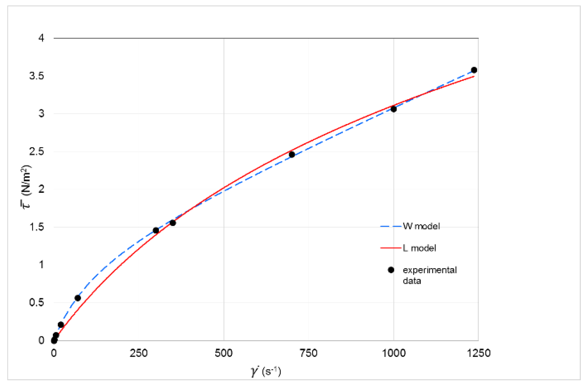
Figure 2 shows the experimental data and the approximating curves for the model of Williamson (W) and the logarithmic model (L); for low values of $\dot{\gamma }$, the model L gives minor values for $\overline{\tau }$ of the model W, and therefore a higher velocity can be expected at the axis of the layer.

Figure 2. Microgel-free xanthan polysaccharide dissolved in a saltwater (salinity = 5 g/L NaCl, temperature = 30 °C); experimental data [11] fitted by W and L models.

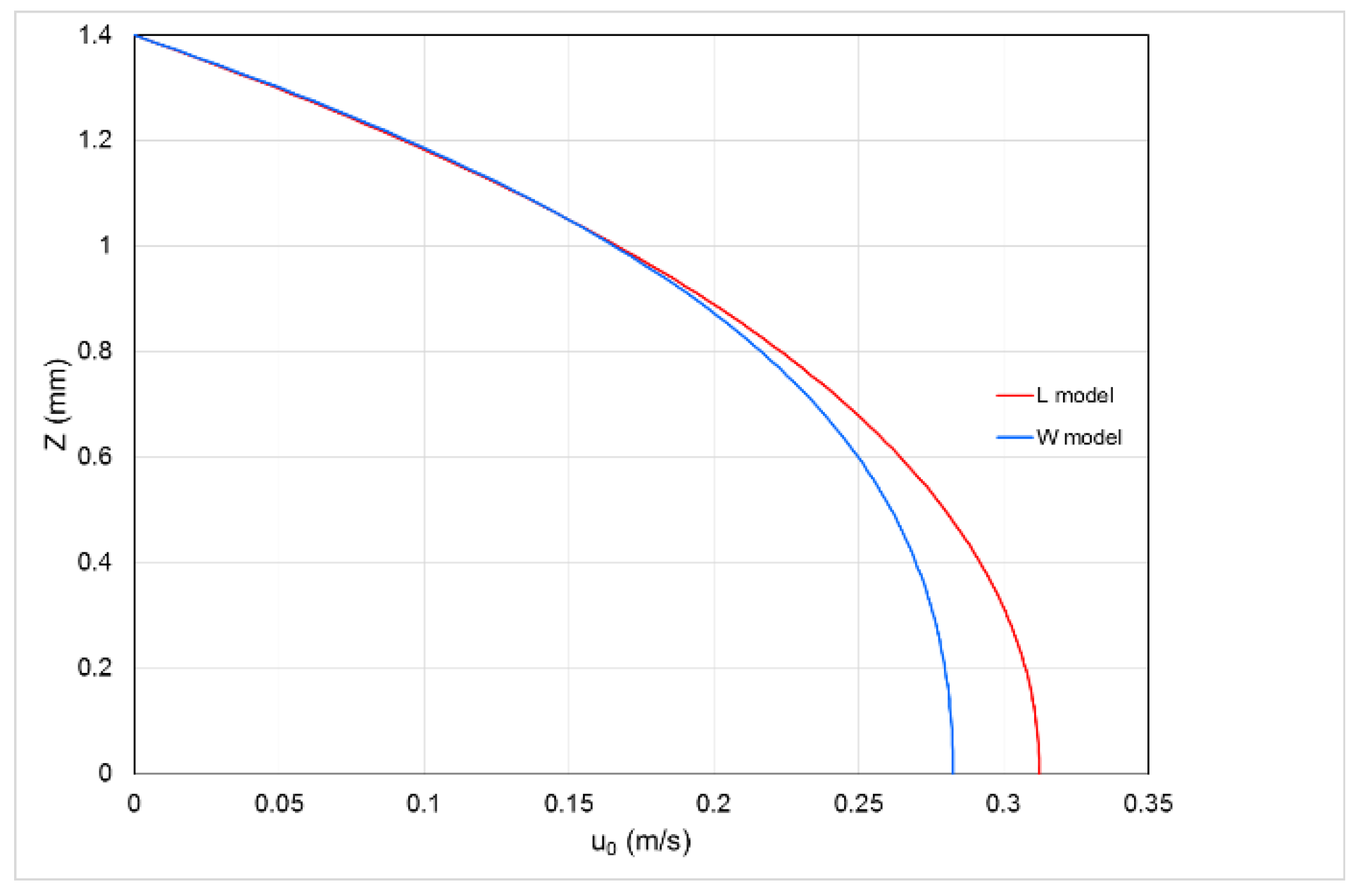
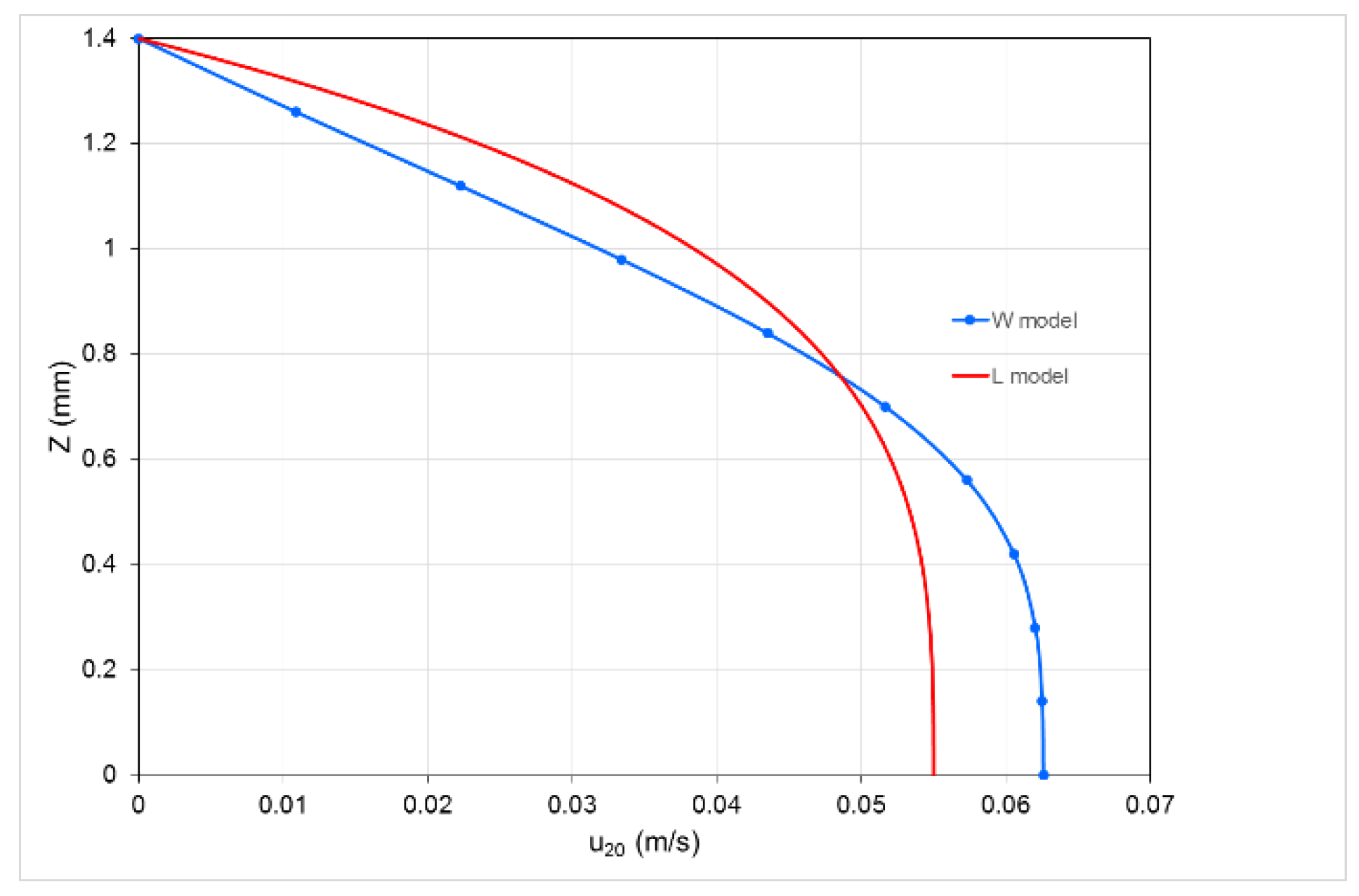
Figure 3 shows the velocity profile in a steady state. As expected, the L model gives rise to a stationary component of the axis velocity greater by about 10% compared to the one given by the model W.

Figure 3. Steady component of velocity for W and L models.

The stationary flow rate, which is the most relevant data, differs in the two cases only by 3%.

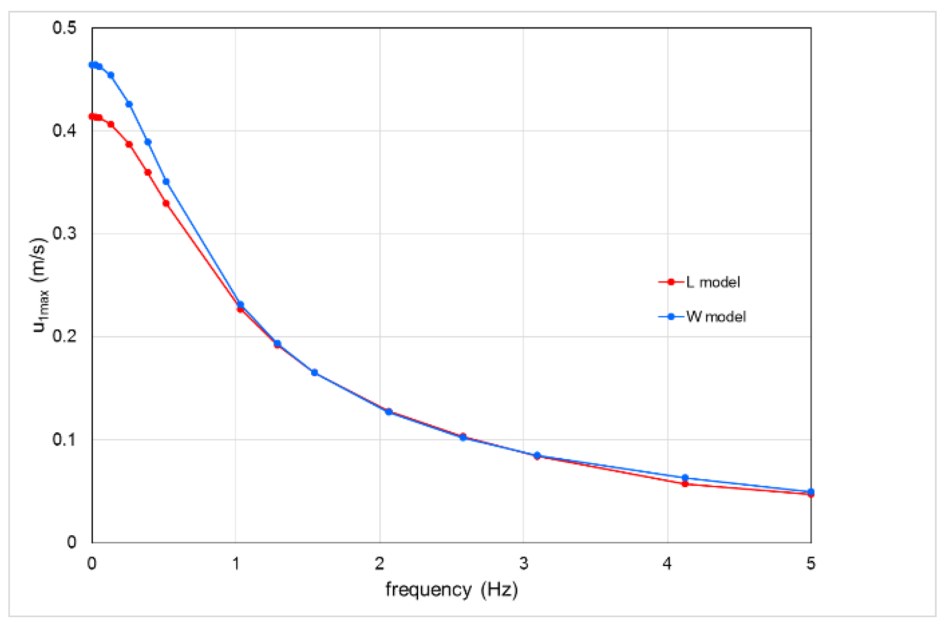
Figure 4 shows, as a function of frequency, the first approximation speed evaluated on the axis, for both models. For low frequencies (<1 Hz), the W model gives higher values than the L model, with differences within 10%. It should be noted that the velocity $u_1$ is less important, because it does not give rise to a flow rate in the period.

Figure 4. First-order velocity amplitude at the layer axis as a function of the frequency of disturbance for L and W models.

Figure 5 shows the steady component of the second-order approximation velocity $u_{20}$, for a frequency $f=0.25$ Hz. Unlike the steady component, in the central part of the layer the W model gives a higher velocity than the L model, while in the zones towards the wall the L model gives a higher velocity. This is due to the great slope of the $\dot{\gamma }-\overline{\tau }$ curve relative to the W model, compared to that of the L model for low values of $\dot{\gamma }$ (i.e., near the layers axis, see Figure 2), which therefore increases the effects of the non-linearity. 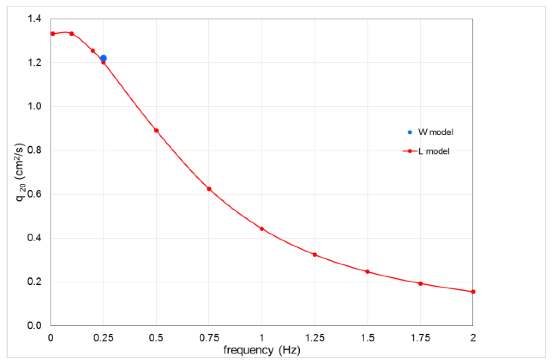The opposite happens near the wall, where $\dot{\gamma }$ is higher and the slope of the $\dot{\gamma }-\overline{\tau }$ is greater in the L model. The stationary rate of flow $q_{20}$, given by the two models for a frequency $f=0.25$ Hz, is practically the same (difference < 2%) as shown in Figure 6, where the second approximation stationary flow rate, calculated with the L model as a function of frequency, is plotted, together with the value given by the model W for $f=0.25$ Hz [9].

Figure 5. Second-order steady velocity: frequency of disturbance 0.25 Hz, ε = 0.25 for L and W models.

Figure 6. Discharge as a function of the frequency for the L model; the dot shows the value of discharge for the W model for f = 0.25 Hz [9].

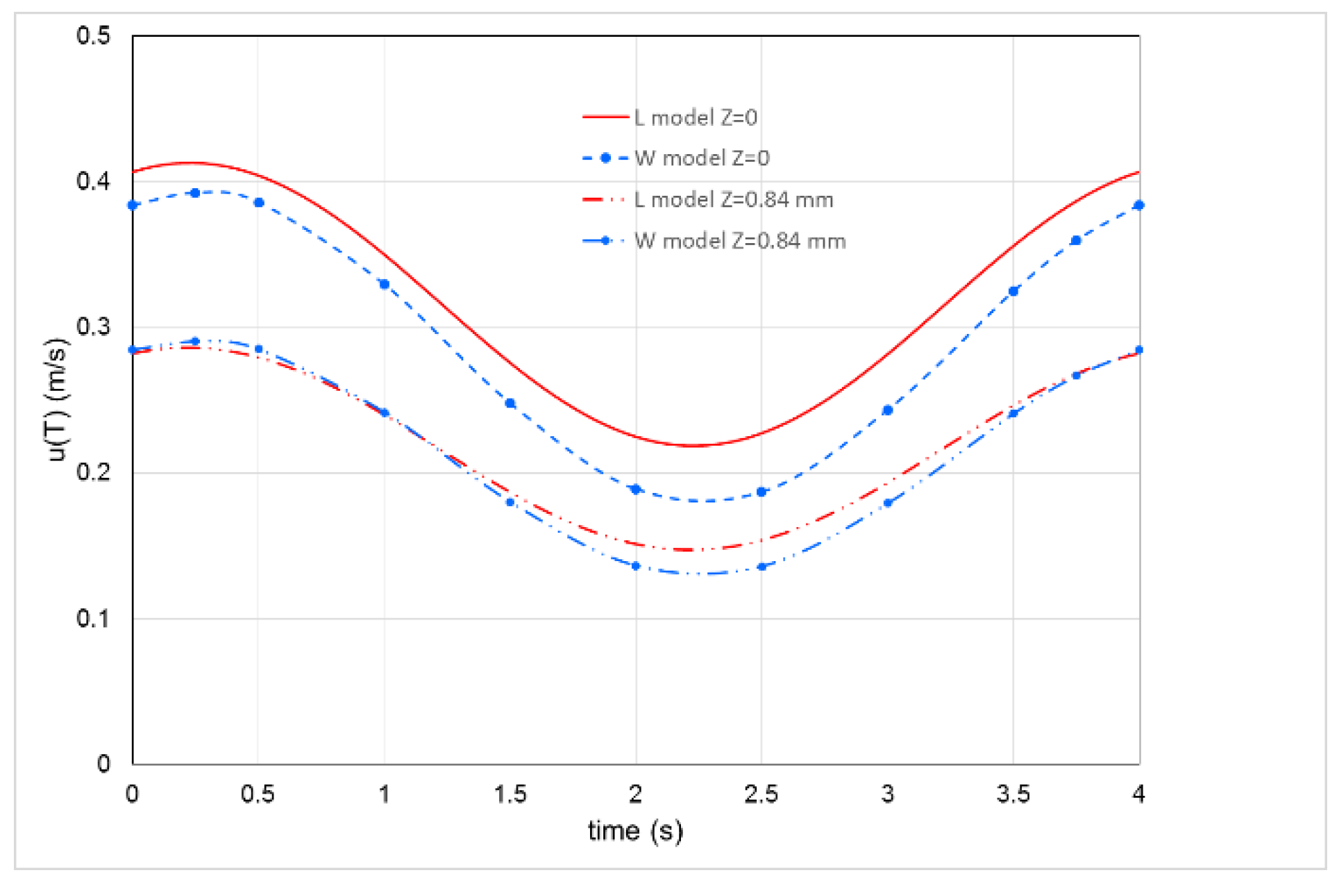
Figure 7 shows the velocity at the axis and at $Z=0.6\delta$ as a function of time, for $f=0.25$ Hz and $\epsilon =0.25$, taking into account the components $u_0$, $u_1$ and $u_{20}$: $u=u_0+\epsilon u_1+{\epsilon }^2{u}_{20}$. As foreseeable by the velocity profiles in Figure 3, the L model always gives a higher value at $Z=0$, while for $Z=0.6\delta$ the differences between the two models are considerably reduced.

Figure 7. $u_0+\epsilon u_1+{\epsilon }^2{u}_{20}$ at layer axis and at Z = 0.6δ as function of time (frequency of disturbance 0.25 Hz, $\epsilon =0.25$).

From a mathematical point of view, the L model is simpler than the W model; the latter requires the calculation of complex index Bessel functions, while the L model makes use of the Kelvin functions of integer order (0 and 1), which are easily calculable and also tabulated, e.g., in the handbook of Abramowitz and Stegun [12]. From a fluid mechanics point of view, to judge which of the two models is more suitable it would be necessary to have available experimental data, which the authors however have not been able to find in the literature. Both models do not take into account the roughness of the walls, which probably should produce a decrease in the flow rate. The effect of roughness, however, according to the authors, could be highlighted only by adopting a numerical solution.

5. Conclusions

The velocity field for a pulsatile flow of a non-Newtonian fluid in a rock fracture has been described using an approximate analytical expression. A two-parameter logarithmic model has been chosen to describe the rheological behavior of the fluid. The fracture has been schematized by two parallel smooth plates; this scheme gives reliable results if the normal stress is less than ~10 MPa and if the aperture variation along a flow path is not large. The solution, carried out up to the second order of approximation, is expressed as a power series expansion of the amplitude of the pulsatile component of the pressure gradient. A numerical example is made using the same fluid and the same geometry of a previous work by the authors, in which the fluid was represented with a three-parameter Williamson model in order to compare the results provided by the two models.

From the comparison, there results that the values of the mean flow rate in a period given by two different models are almost identical, even in the case in which the amplitude of the perturbation ε is a quarter of the steady component. The velocity profiles are quite different; in particular, the velocity near the axis is higher for the L model (with a maximum deviation of 10% on the axis), since the apparent viscosity at low shear rate given by the L model is lower than that provided by the W model, as shown in Figure 1.

The authors believe that it is essential to have several rheological models to test, because it is not possible to know a priori what will best represent the experimental data. They therefore consider the introduction of this particularly simple rheological model to be justified and useful.