Comparison of Diatom Paleo-Assemblages with Adjacent Limno-Terrestrial Communities on Vega Island, Antarctic Peninsula

Abstract

Diatoms are useful ecological and paleolimnological indicators routinely used to reconstruct past conditions and monitor environmental change. Despite this, diatom assemblages from lake sediment cores are often difficult to interpret due to a limited knowledge of the ecology of some species, some of which may originate from the adjacent limno-terrestrial landscape. Here, we compare diatom assemblages from two recently published Antarctic lake sediment cores collected from the northeast and southwest sides of Vega Island, Antarctic Peninsula. We further compare the sediment core assemblages with adjacent modern communities inhabiting four different limno-terrestrial habitat types to gauge the importance of landscape connectivity in determining paleo-assemblage structure. We found that diatom assemblage composition was significantly different between the two cores, and our survey of modern habitats further revealed habitat type to be an important factor determining the composition of limno-terrestrial samples. Differences in modern habitats were driven primarily by Chamaepinnularia krookiformis in mosses, Nitzschia paleacea in ponds, and Fistulifera pelliculosa in streams. When modern communities were compared with paleo-assemblages through ordination, the cored lake from the northeast side, which exhibited greater hydrological connectivity with its surroundings, clustered more closely with the adjacent modern samples. Meanwhile, the cored lake from the southwest side, which was more hydrologically isolated, formed a distinct cluster separate from the others. Overall, species richness and diversity were greater on the southwest side of the island than the northeast, and the known distributions of diatom taxa supported the notion that Vega Island was a transitional zone between the Maritime and Continental Antarctic bioregions. These results collectively suggested that while environmental and spatial controls may be influential in determining diatom community composition, the unique hydrogeological setting of individual waterbodies was an important consideration for determining the assemblage structure of lake cores. This paper furthermore expanded ongoing research of diatom diversity and distributions on maritime Antarctic islands, which will improve diatom-based interpretations for regional ecological monitoring and paleolimnology in the future.

1. Introduction

Climate change has had an impact on the entire planet, but it has had a disproportionate impact on the Polar Regions. Apart from melting glaciers and ice sheets, which provide some of the most unambiguous and visible evidence of climatic disequilibrium [1,2], Antarctic freshwater habitats, such as lakes and ponds, also reflect changes within their simplified food webs and provide a detailed record of these changes within their sediments [3,4]. In Antarctica, many of the most important changes are connected with liquid water availability, which is made possible through subtle increases in temperature [5]. Changes in the distribution of liquid water influence the abundance and connectivity of certain habitat types, as well as ionic concentrations and salinity through concentration and dilution, e.g., [6]. Furthermore, the predicted expansion of Antarctic ice-free areas is likely to promote regional-scale biotic homogenization [7], leading to the extinction of less competitive species and even spread invasive taxa. More detailed studies of these sensitive areas are needed [8], especially in regard to the drivers of biological diversity and their responses to climatic pressures.

Diatoms (Bacillariophyceae) are single-celled eukaryotic organisms with the ability to photosynthesize and occupy almost every known moist or aquatic environment [9]. Their cells contain a yellow-brown pigment, which is stored in a silica capsule that is uniquely ornamented for each species, allowing for relatively straightforward morphological identification [9]. The species-specific response of diatoms to changes in their physical and chemical environment, as well as high preservation potential in sediment made diatoms good environmental proxies for paleoecological/paleoenvironmental reconstructions and environmental monitoring [10]. As a result, diatoms are widely used in environmental and biogeographical studies, especially in Antarctica [11], where they are one of the best represented eukaryotic lineages. Previous work has split Antarctica into three main biogeographical regions based on their differences in flora and fauna [12] and include Continental Antarctica, Maritime Antarctica (i.e., the Antarctic Peninsula), and Sub-Antarctica (the outlying islands). Given that the ability of diatoms to be reliably used as bioindicators is dependent on accurate taxonomic assignment, it is noteworthy that a taxonomic revision was recently performed for the diatom flora of the Maritime Antarctic region [13], which includes the James Ross Island Archipelago in the northeast Antarctic Peninsula (AP). Thus, this area represents an ideal location for studies of diatom ecology and long-term ecological monitoring.

Most diatom reconstructions from lake sediment cores have been performed in East Antarctica [14,15,16,17,18,19,20], with fewer records from the AP area, e.g., [21]. However, paleolimnological work has been recently conducted on Vega Island [22,23,24,25], with two studies in particular, Píšková et al. [26] and Čejka et al. [27], providing some of the first high-resolution data on the abundance, diversity, and structure of diatom paleo-assemblages from the island. Specifically, Píšková et al. [26] provided a multi-proxy analysis of Lake Esmeralda, which is situated on the southwest side of the island and has recently become hydrologically isolated, while Čejka et al. [27] studied Lake Anónima, which is a flow-through lake on the northeast side. Diatom assemblages from Antarctic lake sediment cores can be difficult to interpret, largely due to the poorly documented ecology of many recovered species [28]. This dilemma may be caused in part by the influx of diatoms from other habitats that may enter lakes from the adjacent terrestrial habitats, such as through landslides and Aeolian redistribution [29]. Furthermore, different diatom species may enter lakes through transport and subsequent sedimentation by stream habitats that empty into lake systems [30], as well as moss and seep habitats that may occupy littoral habitats at lower lake levels, e.g., [31]. For example, Píšková et al. [26] found one species of diatom, Microcostatus australoshetlandicus, to exhibit a high abundance, though very little is known about its ecology given its documented rarity throughout the region.

Different diatom habitat types such as ponds, mosses, streams, and seepages are important indicators of Antarctic climate change [32,33,34] and have been previously shown to harbor different communities on the sub-Antarctic islands [35,36] and in Maritime Antarctica [34,37,38]. For example, on Ulu Peninsula, James Ross Island (JRI), significant differences in diversity were found among different habitat types, with ponds being more diverse than seepages and streams [39]. These differences may arise from the distinct abiotic pressures characteristic for individual habitat types. For example, stream diatom communities are strongly influenced by flow regime [30,40,41,42], and research on East Antarctica has previously linked long-term hydrological differences to the biogeographical distributions of individual taxa [40]. On the other hand, moss and seepage communities may be better adapted to frequent desiccation and exposure, as they are often composed of heavily silicified taxa commonly found in terrestrial habitats [34,38]. Understanding the diversity of these adjacent habitat types may substantially advance our understanding of the ecological preferences of terrestrial and lacustrine diatoms to improve environmental interpretations of subfossil and fossil assemblages in sediment records.

In this study, our main aim was to compare and contrast the sediment core diatom communities taken from lakes Anónima and Esmeralda and compare them with corresponding, adjacent freshwater and terrestrial habitat types to improve our understanding of how these assemblages may have formed. To do this, we assessed the differences between four different habitat types (ponds, streams, mosses, and seeps) taken from two sides of Vega Island, northeast AP: Cape Lamb (hosting Lake Esmeralda) and Devil’s Bay (hosting Lake Anónima). We hypothesized that Lake Anónima, given its greater hydrological connectivity with the surrounding landscape, would have diatom assemblages more similar to the adjacent terrestrial and aquatic habitat types than Lake Esmeralda, which is more hydrologically isolated. We further predicted that the four different habitat types would harbor different diatom communities due to the different abiotic requirements of different diatom taxa, as described in previous studies, e.g., [34]. We predicted that diatom assemblages differed between northeast and southwest Vega Island due to local environmental controls, including water body connectivity, and orographic barriers to dispersal.

2. Materials and Methods

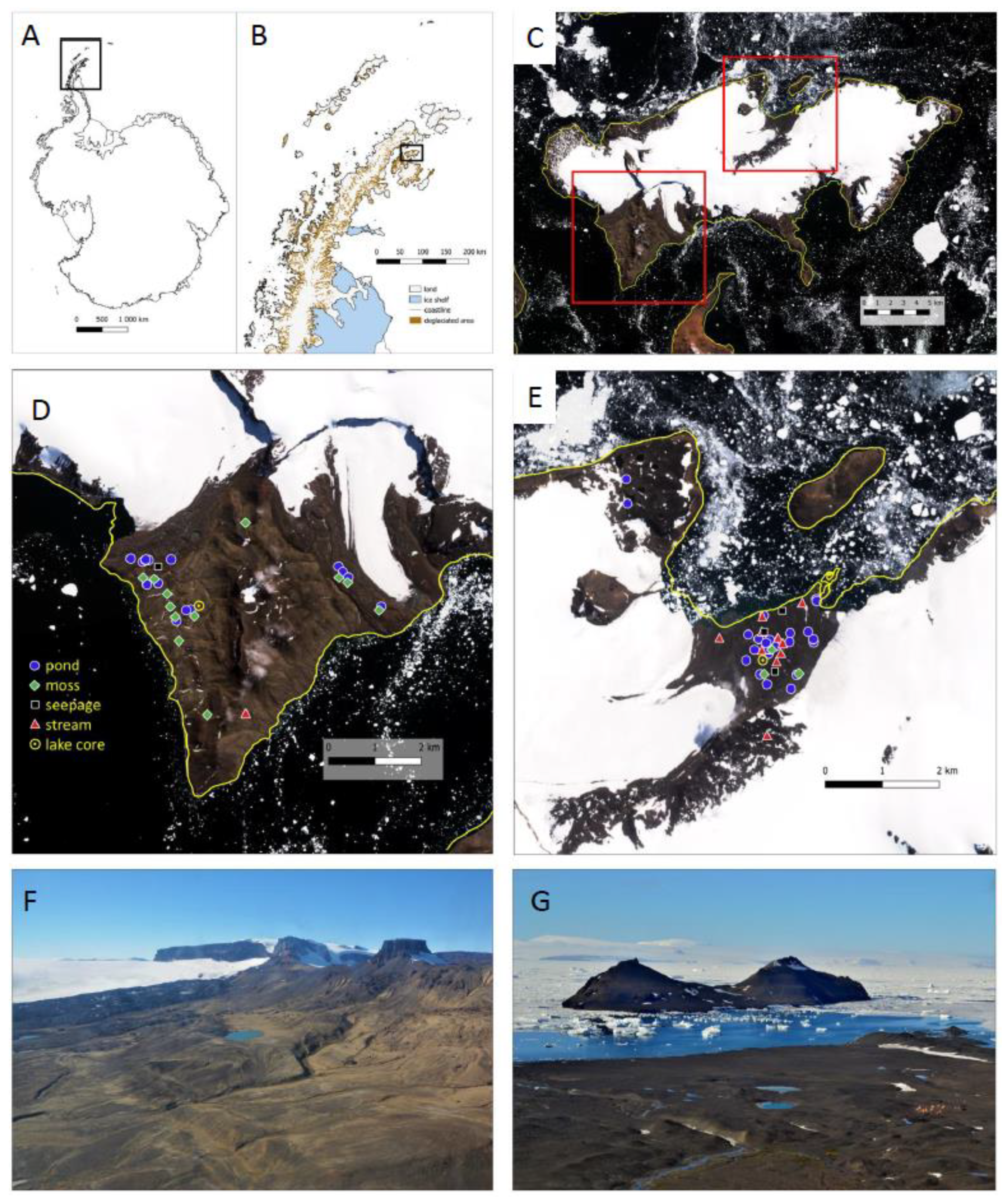
2.1. Site Description

Vega Island is located at the northeast (NE) side of the AP (Figure 1A,B) and was discovered in October of 1903 by the Swedish Antarctic Expedition led by Swedish geologist Otto Nordenskjöld and captain Carl Anton Larsen. The climate of Vega Island is cold and semi-arid. The mean annual air temperature at the J. G. Mendel Station on northern JRI (~25 km to the west) was −7.0 °C over the period of 2006–2015, with summer daily maxima exceeding +10 °C and winter minima dropping below −30 °C [43]. Interannual temperature variability is strongly related to the extent and persistence of sea ice, which affects the air temperature above the low-lying and coastal areas [44]. The entire James Ross Island Archipelago is situated in the precipitation shadow of the AP with annual precipitation between 300 and 500 mm of water-equivalent [45,46]. However, a significant proportion of snow is blown away from flat and concave surfaces, thus limiting its contribution to soil moisture [47]. The highest point of the island lies at 630 m above sea level (a.s.l.).

The oldest rocks exposed on Vega Island are Late Cretaceous sandstones, mudstones, and conglomerates of the Santa Marta, Snow Hill Island, and López de Bertodano formations [48]. The elevated volcanic mesas in the surrounding area are formed by basaltic to trachybasaltic rocks [49,50] of the Miocene to Pleistocene James Ross Island Volcanic Group [51,52]. The mostly subglacial volcanic setting has produced a specific morphology, including steeply-inclined hyaloclastite breccia foresets covered by flat topsets of subaerial basalt lavas [53]. A minor amount of subaquatic eruptions is represented on Vega Island by tuffs and lapilli tuffs [53]. The ice-free areas are covered by till and glaciofluvial sediments emplaced here after the retreat of local glaciers and by marine sediments in coastal areas [27,54]. The island terrestrial flora is composed of a limited number of bryophytes and lichens due to the scarcity of liquid water [55].

Cape Lamb (63°54′ S, 57°37′ W) forms the southwest (SW) tip of Vega Island (Figure 1C,D). It is the largest ice-free area on the island, with a maximum elevation of 482 m a.s.l. The outcrop consists of Cretaceous–Miocene sediments and volcanic rocks [56,57]. Streams of this area are shallow, carry clay and silt, and often change course and catchments because of fluvial erosion [23,26]. The most prominent lake here, Lake Esmeralda (63°50′ S; 57°25′ W, Figure 1F), is situated at an altitude of 68 m a.s.l. The lake is endorheic and is a maximum of 6 m deep. Catchment streams are acidic (pH = ~4); however, Cape Lamb lakes reach an average pH of 9.17 (10 samples), and the pH of Lake Esmeralda was 5.5 when marginal measurements were taken during 2014 and 2017 [26]. Lake Esmeralda disconnected with meltwater inflow in the recent past (~230 years ago) due to fluvial erosion, and precipitation is now the dominant source of water to the lake [23,26]. Salt crusts in the catchment surface indicate higher lake levels in the past [26,58]. The lake adjoins a slope above the entire lake catchment with basalt boulders and hyaloclastite breccia. The lake core recovered from Lake Esmeralda, named ESM3, was roughly 177 cm long; however, diatoms were only recovered from the top ~25 cm, encapsulating a period of ~200 years [26].

Devil’s Bay (63°49′ S, 57°19′ W) is located on the northeast (NE) part of Vega Island (Figure 1C,E). The ice-free area of Devil’s Bay is surrounded by adjacent dome glaciers on volcanic mesas with some outlets including the Bahía del Diablo Glacier [59], and the mean annual air temperature over the period 2000–2002 was −5.5 °C [60]. The most prominent lake at Devil’s Bay is Lake Anónima (63°49′20′′ S, 57°19′30′′ W, Figure 1G), which lies 24 m a. s. l. in the till plain of Bahía del Diablo [59]. It is almost circular with a total surface area of ~2000 m² and a maximum depth of 4.6 m [61]. The lake’s bedrock is formed by Cretaceous sediments of the Marambio Group and is surrounded by elevated volcanic mesas (basalt, hyaloclastite breccia) [52,53]. The ice in the till plain dams the lake and melts seasonally, causing fluctuations in the water level (~1 m), as well as promotes underground drainage into surface streams and the nearby lake systems. Thus, the lake can be regarded as through-flow [27,61]. The lake core recovered from Lake Anónima was 69 cm long, named AN13, and dated to encapsulate >2000 years [27]. The pH at the margin of Lake Anónima measured 8.9 during January 2013, and the average pH of lakes from Devil’s Bay was 9.27 (24 samples).

2.2. Sampling of Modern Habitats

A total of 113 samples were collected from four different habitat types (ponds, mosses, streams, seepages) on the two ice-free areas of Vega Island (Figure 1C,D), during the austral summers of 2013 (Devil’s Bay) and 2014 (Cape Lamb) (Table S1). From all habitat types (except mosses, which were directly transferred into tubes), samples were collected by removing the upper layer of submerged littoral sediments and rocks, placing them in a clean plastic vial, and immediately fixing them with 96% EtOH. Samples were then transported to the Department of Ecology at Charles University (Prague, Czech Republic).

2.3. Slide Preparation and Sample Analysis

Samples for morphological diatom analysis (for both sediment cores and modern material) were prepared following the method described in van der Werff [62]. First, samples were cleaned by adding 37% H₂O₂ and heated to 80 °C for 1 h, followed by the addition of KMnO₄ to complete the reaction. After digestion, samples were rinsed three times with deionized H₂O and centrifuged (3 × 10 min at 3700× g). The material was diluted with distilled water to avoid excessive concentrations of diatom valves, dried onto microscope cover slips, and mounted with Naphrax^® medium onto permanent slides. Samples and slides are archived at the Department of Ecology, Charles University, Czechia, and at the Meise Botanic Garden, Belgium.

In each sample, four-hundred valves were enumerated on random transects at 1000× magnification under oil immersion using an Olympus BX43 microscope, equipped with Differential Interference Contrast (Nomarski) optics and an Olympus DP27 camera using the cellSens Entry Imaging Software. Valve dimensions (length (L), width (W), and stria density (S)) were determined on every species to compare with published values to be certain of taxonomic classification. The work of Zidarova et al. [13] was used as the main source of taxonomic identification. For several specimens, identification to the species level was not possible, and in such cases, it is listed using designations “cf.” or “sp.” For Antarctic species, the geographic distribution was subdivided into sub-Antarctic (SA), Maritime Antarctic (MA), and Continental Antarctic (CA) regions based on Zidarova et al. [13]. To put biogeographical results into context, geographic distributions of Vega Island diatoms were compared with James Ross Island and Livingston Island using data from Kopalová [63]. Diatoms from both sediment cores and modern communities were identified and counted by the same analyst (M. Bulínová).

2.4. Statistical Analysis

To compare diatom assemblage structure among different habitat types and between sediment cores taken from the two sides of the island, diatom counts were transformed to relative abundances (% of total diatom valves counted per sample), and species richness (S), the Shannon Diversity index (H’, [64]), and evenness (J’, [65]) were calculated. Diversity metrics were visualized with boxplots (lines indicating the median and upper and lower quartiles), and Tukey’s honest significance differences (HSD) and Welch’s t-tests were used to determine significant differences between habitat types and NE/SW sides of the island, respectively.

Relative abundance data were visualized with dot plot diagrams organized by different habitat types and the two sides of the island using the rioja R package [66]. In these plots, a point is generated for each taxon within its corresponding sample that is proportional in size to its relative abundance. In order to better observe relationships between sides and samples, principal components analyses (PCA) were generated. Data were square-root transformed, and PCAs were generated using the vegan package in R [67]. For both dot plot diagrams and PCAs, taxa that did not appear at more than 4% relative abundance in any sample were removed prior to analyses to reduce the influence of rare species.

To test for statistical differences in community structure based on categorical variables, such as differences in habitat and island aspect, we used permutational multivariate analysis of variance (PERMANOVA [68]) using Euclidean distances on the same filtered dataset. To test if diatom communities were different between the different sides of the island, we included only pond habitats, since other habitat types did not provide adequate replication between island sides for evaluation. The significance level was set at α = 0.05, and all analyses and figures were generated using R Version 3.4.3 [69].

3. Results

3.1. Vega Island Diatom Flora and Biogeographic Distributions

We observed 36 genera and 173 species in all the Vega Island samples, including sediment cores and modern surface samples. Almost 43% of all observed Vega Island taxa showed a restricted Antarctic distribution with the majority confined only to the Maritime Antarctic Region, whereas only 19% had a cosmopolitan distribution (

Table 1. Proportion of observed taxa from the entire Vega Island dataset, Devil’s Bay, Cape Lamb, James Ross Island, and Livingston Island exhibiting known biogeographical distributions. When it was impossible to establish correct taxonomical identity, the distribution was designated “unidentified”.

Biogeographic Distribution	Vega Island	Devil’s Bay	Cape Lamb	James Ross Island	Livingston Island
	%	%	%	%	%
Cosmopolitan	19.08	20.93	18.18	29.37	28.37
Maritime Antarctic	41.62	45.74	40.56	38.89	47.52
Unidentified	21.97	16.28	23.08	10.32	9.22
Maritime and Continental Antarctic	5.78	6.98	6.29	7.14	4.26
Maritime and Sub-Antarctic	2.89	3.88	2.8	7.94	9.93
Maritime Antarctic and South America	2.31	0.78	2.8	0	0
Southern Hemisphere	4.05	3.88	3.5	0	0
Continental and Maritime Antarctic and South America	0.58	0.78	0.7	0	0
Maritime, Continental, and Sub-Antarctic (entire Antarctic Region)	0.58	0.78	0.7	0.79	0.71
Marine	0.58	0	0.7	5.56	0

). Furthermore, six percent of the observed species were shared with the Antarctic Continent, 3% with the sub-Antarctic islands, and only less than 1% present within the entire Antarctic Region. The diatom flora of Vega Island was less cosmopolitan than on nearby JRI and Livingston Island (29 and 28%, respectively), and it contained more Maritime Antarctic species than JRI (39%), though less than Livingston Island (48%; Table 1).

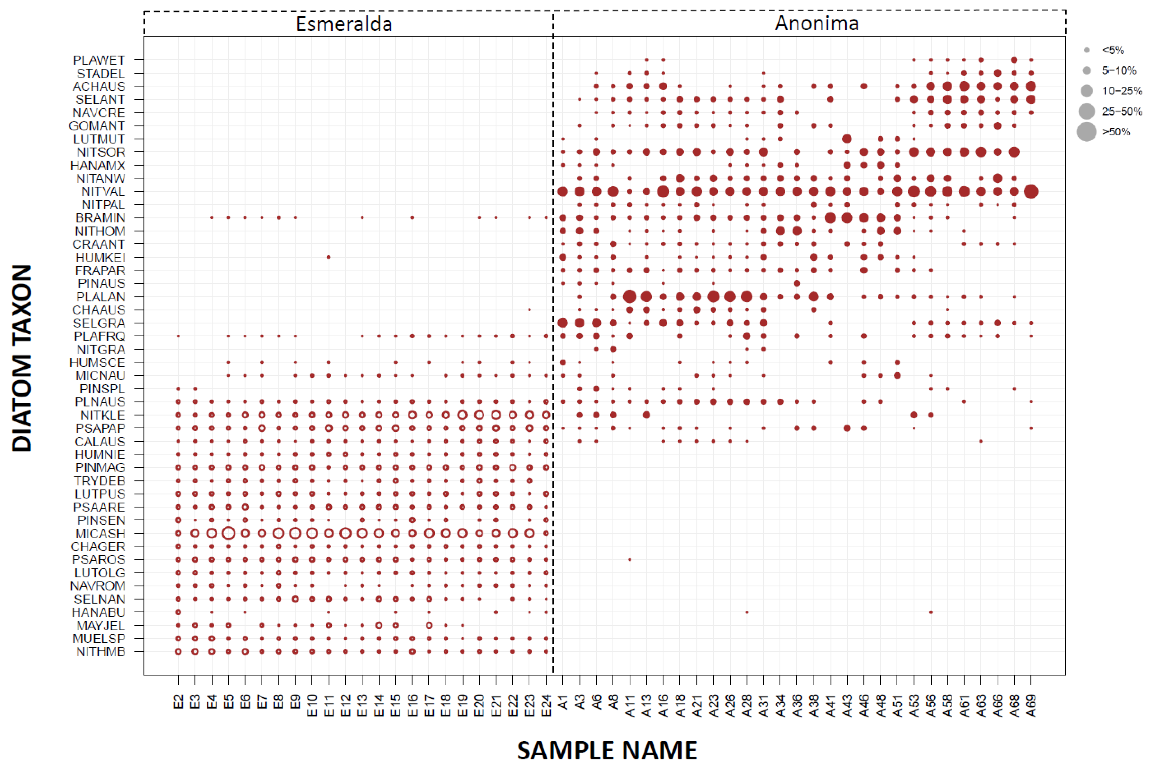
3.2. Paleolimnological Analysis

A total of 86 taxa representing 31 genera were counted in the upper 24 samples of the Lake Esmeralda sediment core (Cape Lamb; Table S2). The most abundant genus in the Lake Esmeralda sediment core was Microcostatus (22%), followed by Psammothidium (16%), Nitzschia (14%), and Pinnularia (11%). In the case of Microcostatus, the genus was mostly represented by a single species, Microcostatus austroshetlandicus, which dominated the entire analyzed section. It was followed by N. kleinteichiana (10%), Psammothidium papilio (6%), and Pinnularia magnifica (6%) (Figure 2). In the Lake Anónima core (Devil’s Bay), eighty different taxa representing 26 genera were counted in 29 samples (Table S2). For the Anónima core, counts were dominated by representatives from the genus Nitzschia (41%), followed by Planothidium (15%), Sellaphora (14%), and Achnanthes (6%), whereas the most abundant species in the Anónima core was Nitzschia velazqueziana, representing 20% of all counted valves. It was followed by Nitzschia soratensis (9%), Planothidium lanceolatum (9%), and Brachysira minor (6%). All other taxa contributed smaller proportions and were more variable (Figure 2).

For both Esmeralda and Anónima cores, the most species-rich genus was Luticola, followed by Pinnularia and Psammothidium in the Lake Esmeralda sediment core and Planothidium in the Lake Anónima sediment core. Of the 132 total species observed from the two sediment cores, only 32 were common to both, and 100 were found in only one of the two lakes. Species that were shared between the lakes were typical lacustrine taxa common for the region such as Psammothidium papilio, Planothidium frequentissimum, and Planothidium australe (Figure 2). The Esmeralda sediment core exceeded Anónima in richness (t-test, t = −11.36, df = 46.19, p < 0.001) and Shannon diversity (t = −6.52, df = 48.36, p < 0.001) (Figure 3). In the Esmeralda core, species richness ranged between 30 and 47 (average = 42), while in the Anónima core, species richness ranged between 12 and 39 (average = 22.9). Shannon diversity values ranged between 2.4 and 3.3 (average = 3.0) in the Esmeralda core, while they were between 0.6 and 0.9 (average = 0.8) in the Anónima core. Differences in evenness were less pronounced between the two lakes (t = −0.43, df = 49.19, p-value = 0.662), though values for Esmeralda were still greater (0.6–0.9; average = 0.8) than those observed in the Anónima core 0.6–0.9 (average = 0.8).

There were no major patterns separating samples within each lake core as a function of age (although, see the discussions in [26,27]), suggesting that the diatom assemblages were relatively uniform throughout the sediment record. When tested with PERMANOVA (999 permutations), the differences between the two cores were significant (pseudo-F = 75.442, p < 0.001).

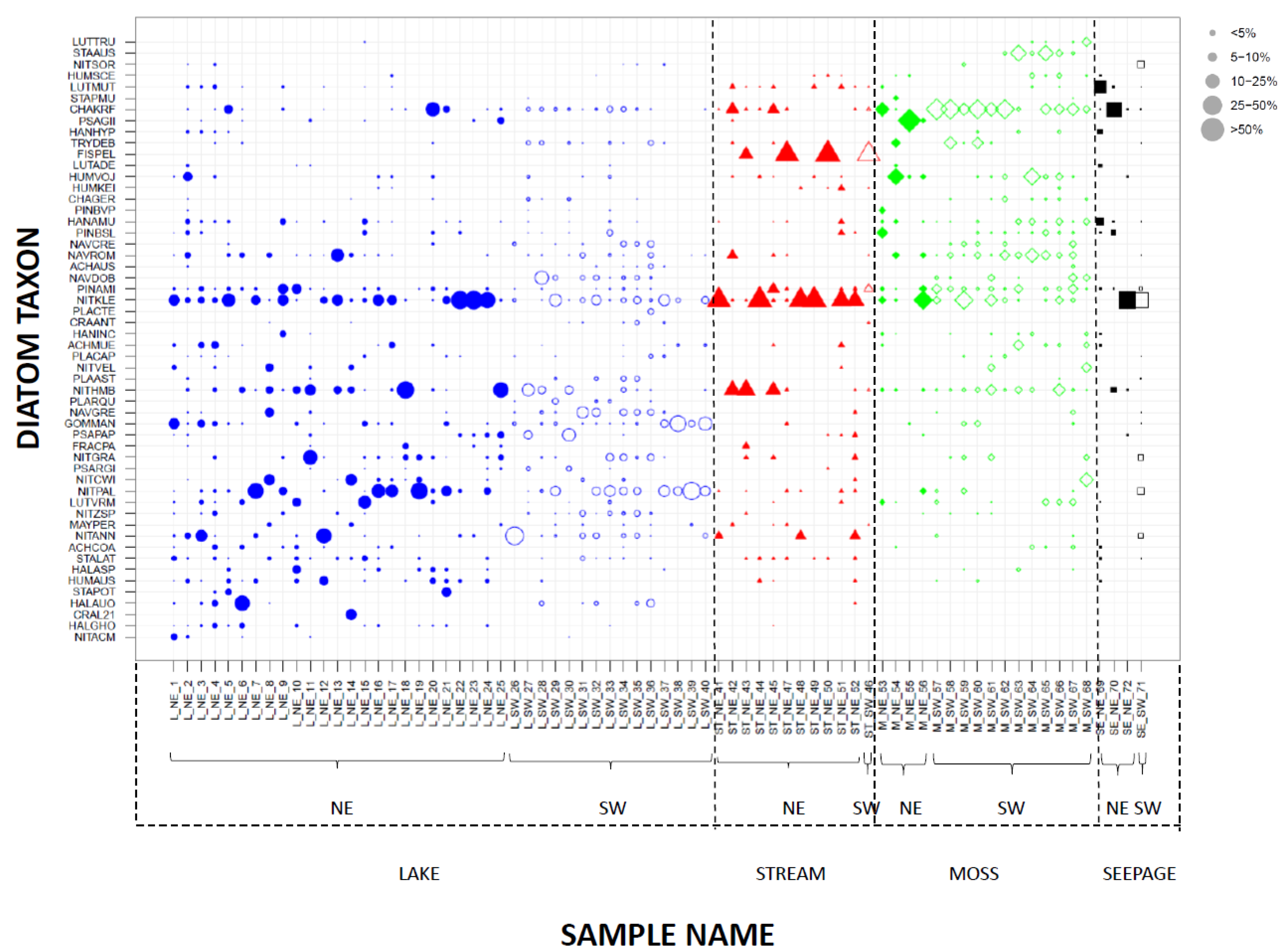
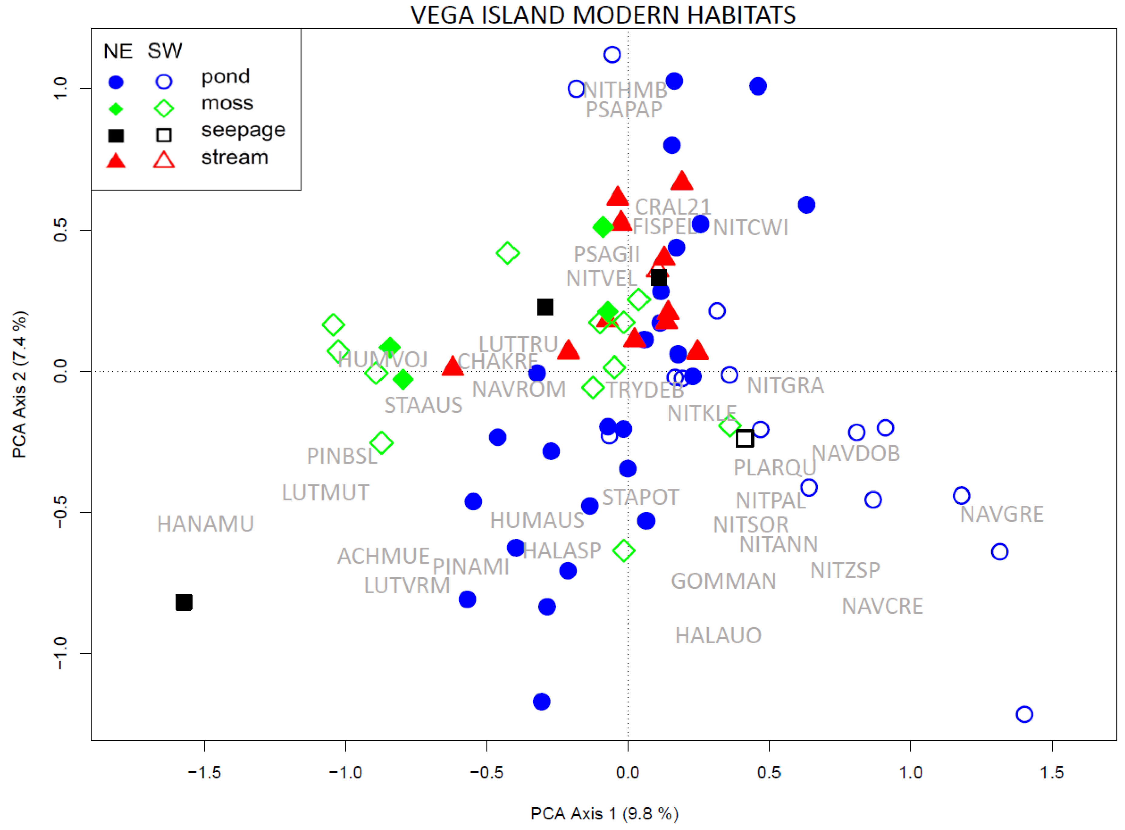
3.3. Species Composition from Modern Habitats

In total, 72 samples from the Vega Island modern material reached the standard quantity of 400 counted diatom valves. From Devil’s Bay, 25 pond, 4 moss, 11 stream, and 3 seepage samples were successfully analyzed, while from Cape Lamb, 15 pond, 12 moss, 1 stream, and 1 seepage samples met the minimum count number. A total of 136 diatom taxa (including species, varieties, and forms) belonging to 31 genera were observed in our study, and a complete list of taxa is presented in Table S2. Due to uncertainties in their correct taxonomic identity, several taxa could only be identified to the genus level, and therefore, their distribution could not be designated (Table S2).

The number of genera recorded per sample ranged from two to 18, with a median value of nine. The highest number of genera was recorded in a lake sample from Devil’s Bay (Sample L_NE_2, 18 genera), and the lowest was found in a stream from the same area (Sample ST_NE_48, 2 genera). The ten most abundant genera accounted for 89.4% of all counted valves, and the ten most common taxa from Cape Lamb accounted for 65.3% of all counted valves from the Cape Lamb dataset. Meanwhile, the ten most common taxa from Devil’s Bay accounted for 68.8% of all counted valves from the Devil’s Bay dataset.

Overall, the most abundant species was Nitzschia kleinteichiana, representing 20.3% of all valves counted, followed by Chamaepinnularia krookiiformis (8.9%), Nitzschia paleacea (8.6%), and Nitzschia homburgiensis (7.8%). The most species-rich genus was Luticola with 23 species, followed by Nitzschia with 11 species. From Cape Lamb, the most abundant taxa were C. krookiiformis (14% of the total relative abundance), N. kleinteichiana (11%), and N. paleacea (10%), while the Devil’s Bay diatom flora was dominated by N. kleinteichiana (26.7%), N. homburgiensis (8.8%), N. paleacea (7.5%), and Fistulifera pelliculosa (6.7%, Figure 4).

Stream habitats were dominated by N. kleinteichiana (38%), F. pelliculosa (23.8%), and N. homburgiensis (11.1%), while mosses were characterized mainly by C. krookiformis (23.7%), N. kleinteichiana (10.6%), and Humidophila vojtajarosikii (7.1%). Seepages were dominated by N. kleinteichiana (38.9%), C. krookiformis (19.3%), and Luticola muticopsis (13.8%). Pond habitats were dominated by Nitzschia species: N. kleinteichiana (17.8%), N. paleacea (14.6%), and N. homburgiensis (9.4%). Considering the two island sides separately, Cape Lamb ponds (SW side) largely consisted of N. paleacea (18.4%), Gomphonema maritimo-antarcticum (10.6%), N. kleinteichiana (10.3%), Nitzschia annewillemsiana (8.4%), and P. papilio (7.4%). Devil’s Bay ponds (NE side) by contrast were dominated by N. kleinteichiana (21.0%), N. paleacea (12.2%), and N. homburgiensis (9.9%) (Figure 4).

For all modern samples combined, species richness ranged between four and 45, with an average value of 16.8. Shannon diversity fluctuated between 3.1 and 0.2, with an average value of 1.6, and evenness ranged from 0.1 to 0.5 with an average of 0.3. Among the four different habitat types (Figure 5), species richness was greatest for lake habitats with an average of 18.5 species and lowest for streams with an average of 12 species. Similarly, Shannon diversity was highest for moss habitats with an average of 1.8 and lowest for streams with an average of 1.1. Lastly, evenness was greatest for moss habitats with an average of 0.6 and lowest for seepages with an average of 0.4. Richness and evenness were not statistically different between sample types when tested with Tukey’s HSD, but Shannon diversity was statistically lower in streams compared with ponds (p = 0.010) and mosses (p = 0.013).

When diversity indices were compared between the two sides of the island across habitat types (Figure 5), Cape Lamb exhibited significantly greater richness (t-test, t = −2.26, df = 62.54, p = 0.028), Shannon diversity (t = −3.20, df = 67.47, p = 0.002), and evenness (t = −2.26, df = 64.09, p = 0.027) than Devil’s Bay. When the diatom diversity of Devil’s Bay was considered alone, species richness per sample ranged from four to 45, with an average of 14.7. Shannon diversity calculated for Devil’s Bay ranged from 0.2 to 3.1, with an average of 1.4, and evenness values ranged from 0.2 to 0.4, with an average of 0.3. When Cape Lamb was considered alone, richness ranged from five to 38 with an average of 20.0, evenness ranged from 0.1 to 0.5 with an average of 0.3, and Shannon diversity ranged from 0.5 to 2.7 with an average of 1.9.

The results of the PCA of the modern samples are summarized in the ordination diagram in Figure 6. The first two axes explain 17.2 % of the total variation in community composition. The x-axis alone explains 9.8% and is (in general) driven by Cape Lamb pond samples to the right and moss samples to the left. The y-axis alone explains 7.4% and is primarily driven by the stream and moss samples at the top of the plot. Nitzschia kleinteichiana is strongly associated with lake samples and Fistulifera pelliculosa with streams. Moss samples are influenced by Humidophila vojtajarosikii and Navicula romanedwardii to the left. Navicula gregaria, N. dobrinatemniskovae, and N. cremeri influence pond samples from Cape Lamb by pulling them to the right of the graph, while Achnanthes muelleri and Luticola vermeulenii pull Devil’s Bay pond samples to the left. When the relationship between diatom community composition and habitat type was tested with PERMANOVA (999 permutations), the differences between habitat types were significant (pseudo-F = 2.917, p < 0.001).

We found that of the 118 species identified from Cape Lamb, thirty four of them were unique to the southwest side of the island (Figure 1). The unique species belonged predominately to the genera Luticola, Planothidium, Psammothidium, and Stauroneis. In contrast, of the 101 species identified in Devil’s Bay, eighteen of them were found to be unique for this side of the island. However, given the unequal frequency of habitat types sampled between the two sides, we focused quantitative comparisons between the two sides of Vega Island on pond habitats alone, since these were the best represented habitats on both sides. Cape Lamb pond communities were largely composed of N. paleacea, G. maritimo-antarcticum, N. kleinteichiana, P. papilio, and N. annewillemsiana. Devil’s Bay ponds were similarly dominated by N. kleinteichiana and N. paleacea, but also N. homburgiensis. When the influence of island aspect on pond communities was tested with PERMANOVA, the individual sides of the island were found to be significantly different (pseudo-F = 3.033, p < 0.001).

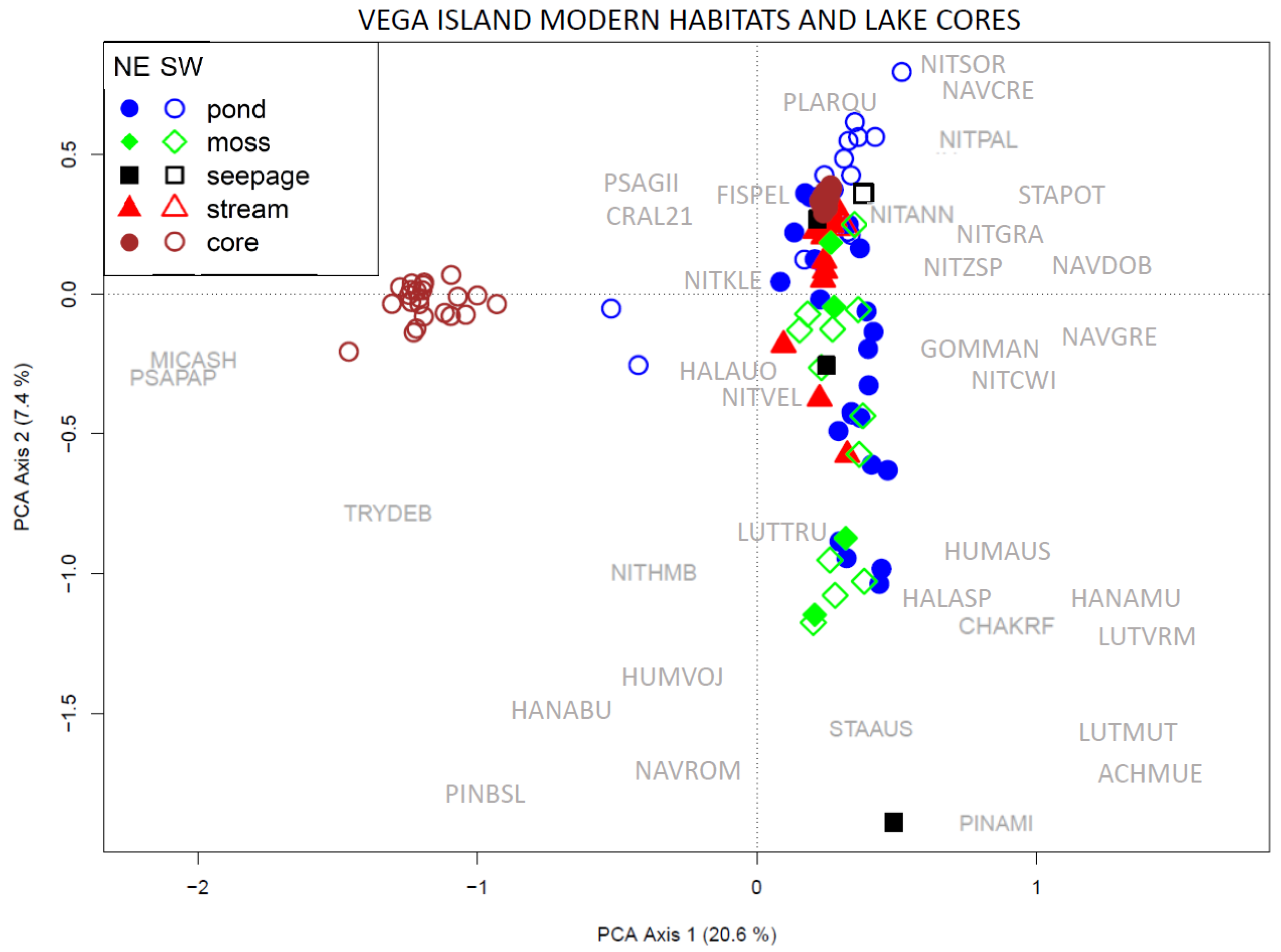
3.4. Comparison of the Entire Vega Island Dataset

Finally, a PCA for the entire dataset from Vega Island is shown in Figure 7. Both axes taken together explained 28% of the variability. The x-axis alone explained 20.6% and was largely driven by Lake Esmeralda to the left, and all other samples to the right. The Lake Esmeralda core, together with the two modern samples from Lake Esmeralda, separated from the rest of the dataset largely because of the influence of one taxon, M. australoshetlandicus. Lake Anónima samples clustered most closely with the modern environments, especially from Devil’s Bay stream habitats. Differences observed within the cores were trivial in the context of the overall variability observed for diatom communities in modern environments, and as a result, core samples clustered tightly together in the ordination.

Species found only in modern material (from both localities) were mainly terrestrial and included Hantzschia incognita, Luticola gigamuticopsis, Mayamaea cf. atomus, and Luticola vermeulenii. Other species included Nitzschia australocommutata, Psammothidium subatomoides, and Nitzschia cf. wilmotteana, which are known mainly from lakes, and Stauroneis australobtusa, known primarily from mosses. Genera only found in modern material were typically represented by only one or a few species, and included Fistulifera, which is common in streams, Geissleria (soils), and Staurosirella (lakes).

Few taxa were found solely in Devil’s Bay and were sparse in both modern habitats and in the sediment record, including Achnanthidium, Orthoseira, Placoneis, and Stauroforma. In Cape Lamb samples (Figure 1), several taxa were specific to the Esmeralda sediment core (beside M. australoshetlandicus) and were not found in the modern material collected from Lake Esmeralda. These included aquatic species Chamaepinnularia elliptica, Sellaphora nana, and Pinnularia strictissima, along with terrestrial species Hantzschia confusa, Luticola katkae, Pinnularia livingstonensis, and Stauroneis minutula. The list is complete with lower abundance of species Fragilariopsis cylindrus, Gomphonema cf. parvulum, Navicula cf. shackletoni, Pinnularia cf. divergens, and Psammothidium manguinii. Furthermore, from Devil’s Bay, several species were found only in the Anónima core. These included aquatic species Adlafia submuscora, Craticula subpampeana, Muelleria aequistriata, Neidium antarcticum, Planothidium wetzelectorianum, Pinnularia australoglobiceps, P. microstauroides, P. splendida, Craspedostauros laevissiumus, and the terrestrial species Stauroneis husvikensis.

4. Discussion

In our paper, we compared published diatom assemblages from Lake Esmeralda [26] and Lake Anónima [27] sediment cores (Figure 1) with modern communities from four adjacent habitats including streams, ponds, mosses, and seepages in Cape Lamb and Devil’s Bay, located on SW and NE Vega Island, respectively. We tested the hypothesis that diatom assemblages from the two lake sediment cores differed from each other and from modern limno-terrestrial habitats due to dynamic hydrologic connectivity on the island. Diatom assemblages from the two lake sediment cores were different from one another, with the Lake Esmeralda sediment core characterized by greater diversity than the Lake Anónima core. The Esmeralda core assemblage was distinct and dominated by Microcostatus australoshetlandicus, which was not present in most other samples from Vega Island, nor elsewhere in the region. Diatom communities from the four habitat types significantly differed from one another in terms of dominant taxa and diversity, and communities from the SW side of the island had greater diversity values than did the NE side. We argue that hydrologic connectivity and habitat type were likely important for structuring diatom assemblages and communities on Vega Island, and further work is needed to explore controls on diatom communities to explain the differences.

4.1. Comparison of Paleo-Material

Here, we holistically analyzed published sites alongside new samples to determine diatom assemblages from different habitats and mechanisms for biogeographic variation. We found that Lake Esmeralda and Lake Anónima had distinctly different diatom assemblages in their sediment cores. There were two major interacting mechanisms that were likely responsible for these differences: The first is that Lake Esmeralda has been recently hydrologically disconnected from the surrounding landscape, thus limiting the potential for allochthonous-derived cells from adjacent habitats to enter the sediment record. Secondly, there were large chemical differences between the two lakes (i.e., pH), which likely was also derived from the differences in hydrological connectivity and was probably a strong environmental filter on which diatom taxa could establish in each lake system. Disentangling which of these was actually responsible for the observed differences (or from potentially other contributing factors, such as dispersal) is more difficult, and answering this question definitively will require further ecological study.

The combined dataset of modern and sediment core diatoms showed that the sediment core diatom assemblages of Lake Esmeralda did not closely resemble any of the recent samples analyzed on Vega Island aside from the recent samples from Lake Esmeralda itself. Interestingly, the uniqueness of this lake’s flora could be attributed primarily to one diatom, Microcostatus australoshetlandicus. This particular species was not observed outside of Lake Esmeralda on Vega Island, and to date, there are no records of this species on JRI, making not only its presence, but indeed its dominance in the lake core a significant observation. The species was originally described based on a small population found in a circumneutral soil sample on Deception Island, a small island belonging to the South Shetland Islands. It was later also observed in algal mats and submerged mosses from small pools on Livingston Island [13] in alkaline pools with a low to moderately high conductivity. The distribution of this unique diatom thus highlighted the hydrological isolation and unique chemistry of Lake Esmeralda in the context of its surroundings.

For Devil’s Bay, while there were some differences between the Anónima sediment core and the modern environments on this side of Vega Island, they were much less pronounced than that described for Lake Esmeralda. One possibility is that Lake Anónima is well-connected to a stream system that facilitates the transport of diatom valves, unlike Lake Esmeralda, whose catchment became isolated ~230 years ago due to river capture [26]. In addition, Lake Anónima exhibits underground drainage into surface streams and the nearby lake systems [27]. Therefore, even if there is no transport of diatom valves, this hydrological exchange may make lake habitats more similar in chemical composition, promoting similar diatom assemblages. Indeed, the Lake Anónima paleo-assemblages cluster somewhere between the recent pond and stream samples, lending support to this interpretation.

It is interesting to note that the species richness was greater in Lake Esmeralda in comparison to Lake Anónima. Given that the diatom record from Lake Anónima covers almost ten times the amount of time [26,27], as well as given the flow-through nature of this lake, which would suggest that species from the surroundings could be transported and deposited there, it is intuitive to think that Lake Esmeralda should have lower diversity values. One possibility is that some of the valves in Lake Anónima were not sufficiently preserved (especially given the more alkaline pH) and thus led to an underestimate of diversity in this lake, while the much younger and more acidic Lake Esmeralda may promote better preservation. On the other hand, the unique setting and hydrochemistry of Lake Esmeralda may enable it to support a greater diversity of species regardless of preservation.

Lastly, it is important to note that samples were collected over different summers, and we cannot rule out the possibility that assemblages may have varied on an inter- or intra-annual basis. However, we argue based on previous work from here and elsewhere in Antarctica that this effect was likely to be small. For example, Kohler et al. [70] investigated diatom communities within Green Creek, McMurdo Dry Valleys, over the course of a summer. While some changes in relative abundances were observed, there were no species that entered or left the community over the course of the summer. Similarly, Stanish et al. [29,40] working in the same region found that while different streams hosted different diatom communities, they were stable from year to year. Finally, in the two lake core papers that provided the basis for this work [26,27], there were no major appearances or extinctions of species in the assemblages over time (although the Anónima core was more variable than Esmeralda). Therefore, while it is likely that the abundances of some species are temporally dynamic, we speculate that diatom flora among sites and habitats are largely static across summers, though we encourage future investigators to perform both seasonal and long-term monitoring to validate this assumption.

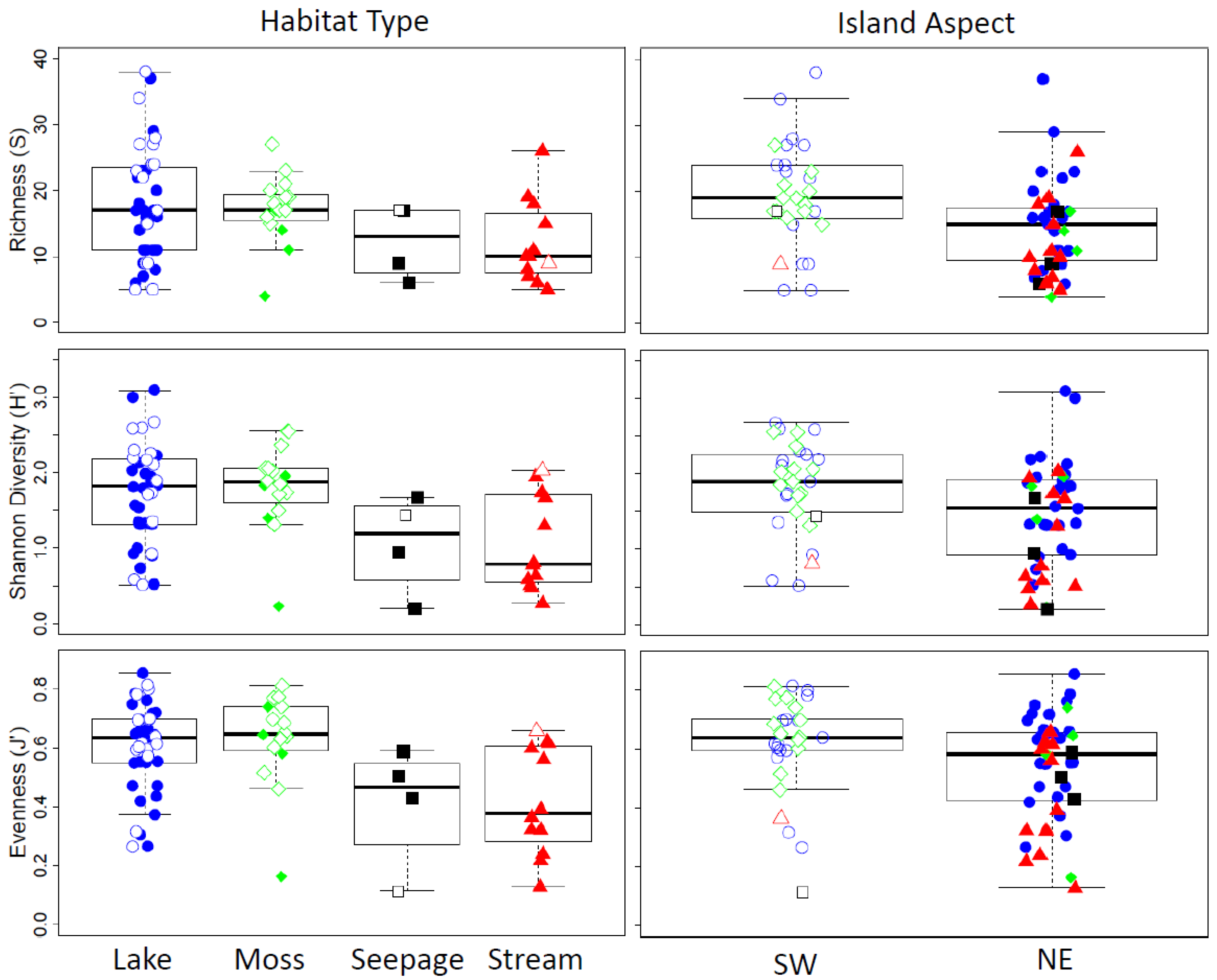
4.2. Influence of Habitat Type

In Antarctica, different habitat types exert strong selective controls on diatom community structure and assemblage due to the environmental conditions they promote and to which they are exposed [11]. For example, the extent and duration of ice cover on lakes and ponds function as the main control in these habitats [71,72,73,74]. Similarly, Antarctic stream communities are greatly influenced by patterns in meltwater generation at their source and are subject to extended periods of desiccation and freezing [30,40,41]. Moisture content is a main control for diatoms living in moss communities [75,76,77], with dry mosses routinely being reported to have fewer species than wet ones, e.g., [35]. Previous work has further shown that the distance to an aquatic source (either freshwater of marine) is more influential than the water’s physico-chemical composition [77]. Seepages, on the other hand, often exhibit higher conductivity and nutrient concentrations than nearby waterbodies [11,39,78,79]. While also ephemeral like Antarctic streams, seeps may provide a more “stable” hydrologic environment given their lower flow rates and thus reduced shear stress and instances of scour. In our study, Vega Island moss and pond habitats were more diverse than streams and seepages, which may reflect the greater relative stability of these former habitat types in contrast to the ephemerally-fed streams and seepages that can potentially exhibit more abrupt changes in aquatic regime.

The submerged aquatic habitats of Vega Island were dominated by the genus Nitzschia, which contrasts with ponds from the sub-Antarctic Islands, where Nitzschia species are less abundant [36]. Additionally, Sakaeva et al. [80] reported only two Nitzschia species from ponds in the McMurdo Sound region near McMurdo Station, none of which were dominant. From stream and pond habitats, three Nitzschia species were common: N. kleinteichiana, N. paleacea, and N. homburgiensis. The first, N. kleinteichiana, is one of the most common Nitzschia species in the Maritime Antarctic Region [13]. It exhibits a broad ecological niche, being found in every habitat investigated [81]. Another Nitzschia species, N. homburgiensis, was also observed at high abundances and has previously been reported from streams in the Maritime Antarctic region [81,82]. Aside from Nitzschia, the small, lightly-silicified diatom Fistulifera pelliculosa was also common in studied streams. This species is commonly observed in other Antarctic streams, e.g., [30], and is hypothesized to be an indicator of high-nutrient areas such as hyporheic upwelling zones [83]. This genus furthermore tolerates unstable flow conditions in streams, including high velocities [84,85], and is probably easily mobilized and transported in the water column from sediments before being deposited to other habitats [30,42].

Diatom communities from Vega Island moss habitats were characterized by species typically reported from Antarctic Peninsula moss samples, such as Chamaepinnularia krookiformis, N. kleinteichiana, and Humidophila vojtajarosikii [13,38]. Humidophila vojtajarosikii is a common species on both JRI and the South Shetland Islands: it has been reported from all of Livingston Island (reported as Diadesmis sp2 in [38]), King George Island, Nelson Island, and Deception Island (Zidarova, personal communication), although rarely exceeding 10% of the total diatom count. The largest populations were found in moist terrestrial to submerged aquatic moss vegetation close to larger lakes [83,86]. Interestingly, the species composition of moss diatoms from Vega Island was substantially different from those recently reported for the nearby Clearwater Mesa [34], which were dominated by Achnanthes muelleri, Hantzschia abundans, and Pinnularia borealis. In limited datasets from seepages, diatom communities were dominated by N. kleinteichiana, the species common in every habitat in the Maritime Antarctic, C. krookiformis (most abundant among wet and moist mosses on the shore of small ponds with elevated salinity and nutrients), and Luticola muticopsis. The latter species is usually the most abundant in terrestrial and aquatic habitats near the coast and influenced by sea birds and sea sprays [13,80].

As observed in the sediment cores, we found that the species richness of modern material from the Cape Lamb side of Vega Island contained a greater number of species than samples from the Devil’s Bay area. Some of these differences may be linked to differences in the number of sampled habitat types between the NE and SW sides of the island (although Devil’s Bay had better representation of different habitats than Cape Lamb) and the fact that some unique species were only represented by one or two valves. On the other hand, differences between pond habitats, which were more comparable in sample size, were statistically different, and future work may do well in investigating if there are indeed differences in the diversity between these two sides of the island and what their drivers might be. One possibility is that there are differences in dispersal potential between the two sides of the island; for example, wind currents coming in the southwest direction from JRI and by the presence of a precipitation shadow formed by the AP, bearing greater influence on Devil’s Bay [59]. Furthermore, differences in conductivity and pH between the two sides of the island are likely to be also an important factor in assembling communities. However, it is important to point out that different waterbodies have specific conditions and histories that have led to their individual assemblage structures, and it is particularly troublesome to make regional generalizations based on an outlier waterbody like Lake Esmeralda. Thus, more study will be necessary to uncover the full ecological past of Vega Island.

5. Conclusions

Our paper brings the first comprehensive picture of the diatom communities inhabiting Vega Island thanks to samples collected on the NE (Devil’s Bay) and SW (Cape Lamb) sides during the summer 2013 and 2014 expeditions. Altogether, 173 taxa were identified belonging to 36 genera, and their known distributions supported the notion that Vega Island was a transitional zone between the Maritime and Continental Antarctic bioregions. Diatom assemblages from the two sediment cores differed substantially from each other in their species composition, richness, and diversity, suggesting different environmental conditions and histories for each lake. For the modern material, habitat type was found to be a major factor in determining diatom community structure, and overall, the diatom flora on Cape Lamb was more diverse than on Devil’s Bay. Lastly, the sediment core assemblages from Lake Anónima were much more similar to adjacent diatom communities than Lake Esmeralda, which likely was because of the greater hydrological connectivity of Lake Anónima with the surrounding landscape. As warmer conditions in the future will likely increase hydrologic connectivity and increase the size and number of (semi)aquatic habitats [87,88], possibly leading to the homogenization of regional diatom distributions [7], the study of how these communities will respond to these changes is now more timely than ever.

References

1. Oerlemans, J. Atmospheric science: Extracting a climate signal from 169 glacier records. Science 2005, 308, 675–677. [Google Scholar] [CrossRef] [PubMed] [Green Version]
2. Cannone, N.; Diolaiuti, G.; Guglielmin, M.; Smiraglia, C. Accelerating climate change impacts on alpine glacier forefield ecosystems in the European Alps. Ecol. Appl. 2008, 18, 637–648. [Google Scholar] [CrossRef] [PubMed] [Green Version]
3. Quayle, W.C.; Peck, L.S.; Peat, H.; Ellis-Evans, J.C.; Harrigan, P.R. Extreme responses to climate change in Antarctic lakes. Science 2002, 295, 645. [Google Scholar] [CrossRef] [PubMed]
4. Laybourn-Parry, J.; Pearce, D.A. The biodiversity and ecology of Antarctic lakes: Models for evolution. Philos. Trans. R. Soc. B 2007, 362, 2273–2289. [Google Scholar] [CrossRef] [Green Version]
5. Gooseff, M.N.; McKnight, D.M.; Doran, P.; Fountain, A.G.; Lyons, W.B. Hydrological connectivity of the landscape of the McMurdo Dry Valleys, Antarctica. Geogr. Compass 2011, 5, 666–681. [Google Scholar] [CrossRef]
6. Roman, M.; Nedbalová, L.; Kohler, T.J.; Lirio, J.M.; Coria, S.H.; Kopáček, J.; Vignoni, P.A.; Kopalová, K.; Lecomte, K.L.; Elster, J.; et al. Lacustrine systems of Clearwater Mesa (James Ross Island, northeastern Antarctic Peninsula): Geomorphological settings and limnological characterization. Antarct. Sci. 2019, 31, 169–188. [Google Scholar] [CrossRef]
7. Lee, J.R.; Raymond, B.; Bracegirdle, T.J.; Chades, I.; Fuller, R.A.; Shaw, J.D.; Terauds, A. Climate change drives expansion of Antarctic ice-free habitat. Nature 2017, 547, 49–54. [Google Scholar] [CrossRef]
8. Jaros, C.L. Temperature-Elevation Effect on Glacial Meltwater Generation in McMurdo Dry Valleys, Antarctica. Ph.D. Thesis, University of Colorado, Boulder, CO, USA, 2003. [Google Scholar]
9. Round, F.E.; Crawford, R.M.; Mann, D.G. Diatoms: Biology and Morphology of the Genera; Cambridge University Press: Cambridge, UK, 1990. [Google Scholar]
10. Smol, J.P.; Stoermer, E.F. The Diatoms: Applications for the Environmental and Earth Sciences, 2nd ed.; Cambridge University Press: Cambridge, UK, 2010. [Google Scholar]
11. Spaulding, S.A.; Van de Vijver, B.; Hodgson, D.A.; McKnight, D.M.; Verleyen, E.; Stanish, L. Diatoms as indicators of environmental change in antarctic and subantarctic freshwaters. In The Diatoms: Applications for the Environmental and Earth Sciences, 2nd ed.; Smol, J.P., Stoermer, E.F., Eds.; Cambridge University Press: Cambridge, UK, 2010; pp. 267–284. [Google Scholar]
12. Chown, S.L.; Convey, P. Spatial and temporal variability across life’s hierarchies in the terrestrial Antarctic. Philos. Trans. R. Soc. B 2007, 362, 2307–2331. [Google Scholar] [CrossRef]
13. Zidarova, R.; Kopalová, K.; Van der Vijver, B. Diatoms from the Antarctic Region: Maritime Antarctica. In Iconographia Diatomologica; Lange-Bertalot, H., Ed.; Koeltz Botanical Books: Schmitten, Germany, 2016; Volume 24, pp. 1–509. [Google Scholar]
14. Fulford-Smith, S.P.; Sikes, E.L. The evolution of Ace Lake, Antarctica, determined from sedimentary diatom assemblages. Palaeogeogr. Palaeoclimatol. Palaeoecol. 1996, 124, 73–86. [Google Scholar] [CrossRef]
15. Roberts, D.; McMinn, A. A weighted-averaging regression and calibration model for inferring lakewater salinity from fossil diatom assemblages in saline lakes of the Vestfold Hills: A new tool for interpreting Holocene lake histories in Antarctica. J. Paleolimnol. 1998, 19, 99–113. [Google Scholar] [CrossRef]
16. Roberts, D.; McMinn, A. A diatom-based palaeosalinity history of Ace Lake, Vestfold Hills, Antarctica. Holocene 1999, 9, 401–408. [Google Scholar] [CrossRef]
17. Roberts, D.; van Ommen, T.D.; McMinn, A.; Morgan, V.; Roberts, J.L. Late-Holocene East Antarctic climate trends from ice-core and lake-sediment proxies. Holocene 2001, 11, 117–120. [Google Scholar] [CrossRef]
18. Roberts, D.; McMinn, A.; Cremer, H.; Gore, D.B.; Melles, M. The Holocene evolution and palaeosalinity history of Beall Lake, Windmill Islands (East Antarctica) using an expanded diatom-based weighted averaging model. Palaeogeogr. Palaeoclimatol. Palaeoecol. 2004, 208, 121–140. [Google Scholar] [CrossRef]
19. Cremer, H.; Gore, D.; Hultzsch, N.; Melles, M.; Wagner, B. The diatom flora and limnology of lakes in the Amery Oasis, East Antarctica. Polar Biol. 2004, 27, 513–531. [Google Scholar] [CrossRef]
20. Hodgson, D.A.; Verleyen, E.; Sabbe, K.; Squier, A.H.; Keely, B.J.; Leng, M.J.; Saunders, K.M.; Vyverman, W. Late Quaternary climate-driven environmental change in the Larsemann Hills, East Antarctica, multi-proxy evidence from a lake sediment core. Quat. Res. 2005, 64, 83–99. [Google Scholar] [CrossRef]
21. Björck, S.; Håkansson, H.; Olsson, S.; Barnekow, L.; Janssens, J. Palaeoclimatic studies in South Shetland Islands, Antarctica, based on numerous stratigraphic variables in lake sediments. J. Paleolimnol. 1993, 8, 233–272. [Google Scholar] [CrossRef]
22. Sinito, A.M.; Chaparro, M.A.; Irurzun, M.A.; Lirio, J.M.; Nowaczyk, N.R.; Böhnel, H.N.; Nuñez, H. Preliminary palaeomagnetic and rock-magnetic studies on sediments from lake Esmeralda (Vega Island), Anatarctica. Latinmag Lett. 2011, 1, 1–7. [Google Scholar]
23. Moreno, L.; Silva-Busso, A.; López-Martínez, J.; Durán-Valsero, J.J.; Martínez-Navarrete, C.; Cuchí, J.A.; Ermolin, E. Hydrogeochemical characteristics at Cape Lamb, Vega Island, Antarctic Peninsula. Antarct. Sci. 2012, 24, 591–607. [Google Scholar] [CrossRef]
24. Irurzun, M.A.; Chaparro, M.A.E.; Sinito, A.M.; Gogorza, C.S.G.; Lirio, J.M.; Nuñez, H.; Nowaczyk, N.R.; Böhnel, H.N. Preliminary relative palaeointensity record and chronology on sedimentary cores from Lake Esmeralda (Vega Island, Antarctica). Latinmag Lett. 2013, 3, 1–7. [Google Scholar]
25. Irurzun, M.A.; Chaparro, M.A.E.; Sinito, A.M.; Gogorza, C.S.G.; Nuñez, H.; Nowaczyk, N.R.; Böhnel, H.N. Relative palaeointensity and reservoir effect on Lake Esmeralda, Antarctica. Antarct. Sci. 2017, 29, 356–368. [Google Scholar] [CrossRef]
26. Píšková, A.; Roman, M.; Bulínová, M.; Pokorný, M.; Sanderson, D.; Cresswell, A.; Lirio, J.M.; Coria, S.H.; Nedbalová, L.; Lami, A.; et al. Late-Holocene palaeoenvironmental changes at Lake Esmeralda (Vega Island, Antarctic Peninsula) based on a multi-proxy analysis of laminated lake sediment. Holocene 2019, 29, 1155–1175. [Google Scholar] [CrossRef]
27. Čejka, T.; Nývlt, D.; Kopalová, K.; Bulínová, M.; Kavan, J.; Lirio, J.M.; Coria, S.H.; Van de Vijver, B. Timing of the Neoglacial onset on the north-eastern Antarctic Peninsula based on lacustrine archive from Lake Anónima, Vega Island. Glob. Planet. Chang. 2020, 184, 103050. [Google Scholar] [CrossRef]
28. Whittaker, T.E.; Hall, B.L.; Hendy, C.H.; Spaulding, S.A. Holocene depositional environments and surface-level changes at Lake Fryxell, Antarctica. Holocene 2008, 18, 775–786. [Google Scholar] [CrossRef]
29. Spaulding, S.A.; McKnight, D.M.; Stoermer, E.F.; Doran, P.T. Diatoms in sediments of perennially ice-covered Lake Hoare, and implications for interpreting lake history in the McMurdo Dry Valleys of Antarctica. J. Paleolimnol. 1997, 17, 403–420. [Google Scholar] [CrossRef]
30. Stanish, L.F.; Nemergut, D.R.; McKnight, D.M. Hydrologic processes influence diatom community composition in Dry Valley streams. J. N. Am. Benthol. Soc. 2011, 30, 1057–1073. [Google Scholar] [CrossRef]
31. Douglas, M.S.V.; Smol, J.P.; Blake, W., Jr. Marked post-18th century environmental change in high-arctic ecosystems. Science 1994, 226, 416–419. [Google Scholar] [CrossRef]
32. Guglielmin, M.; Dalle Fratte, M.; Cannone, N. Permafrost warming and vegetation changes in continental Antarctica. Environ. Res. Lett. 2014, 9, 045001. [Google Scholar] [CrossRef] [Green Version]
33. Gooseff, M.N.; Barrett, J.E.; Adams, B.J.; Doran, P.T.; Fountain, A.G.; Lyons, W.B.; McKnight, D.M.; Priscu, J.C.; Sokol, E.R.; Takacs-Vesbach, C.; et al. Decadal ecosystem response to an anomalous melt season in a polar desert in Antarctica. Nat. Ecol. Evol. 2017, 1, 1334–1338. [Google Scholar] [CrossRef]
34. Kopalová, K.; Soukup, J.; Kohler, T.J.; Roman, M.; Coria, S.H.; Vignoni, P.A.; Lecomte, K.L.; Nedbalová, L.; Nývlt, D.; Lirio, J.M. Habitat controls on limno-terrestrial diatom communities of Clearwater Mesa, James Ross Island, Maritime Antarctica. Polar Biol. 2019, 42, 1595–1613. [Google Scholar] [CrossRef]
35. Van de Vijver, B.; Beyens, L. Biogeography and ecology of freshwater diatoms in Subantarctica: A review. J. Biogeogr. 1999, 26, 993–1000. [Google Scholar] [CrossRef]
36. Van de Vijver, B.; Gremmen, N.; Smith, V. Diatom communities from the sub-Antarctic Prince Edward Islands: Diversity and distribution patterns. Polar Biol. 2008, 31, 795–808. [Google Scholar] [CrossRef]
37. Kopalová, K.; Veselá, J.; Elster, J.; Nedbalová, L.; Komárek, J.; Van de Vijver, B. Benthic diatoms (Bacillariophyta) from seepages and streams on James Ross Island (NW Weddell Sea, Antarctica). Plant Ecol. Evol. 2012, 145, 190–208. [Google Scholar] [CrossRef]
38. Kopalová, K.; Nedbalová, L.; Van de Vijver, B. Moss-inhabiting diatoms from two contrasting Maritime Antarctic islands. Plant Ecol. Evol. 2014, 147, 67–84. [Google Scholar] [CrossRef] [Green Version]
39. Kopalová, K.; Nedbalová, L.; Nývlt, D.; Elster, J.; Van de Vijver, B. Diversity, ecology and biogeography of the freshwater diatom communities from Ulu Peninsula (James Ross Island, NE Antarctic Peninsula). Polar Biol. 2013, 36, 933–948. [Google Scholar] [CrossRef]
40. Esposito, R.M.M.; Horn, S.L.; McKnight, D.M.; Cox, M.J.; Grant, M.C.; Spaulding, S.A.; Doran, P.T.; Cozzetto, K.D. Antarctic climate cooling and response of diatoms in glacial meltwater streams. Geophys. Res. Lett. 2006, 33, 2–5. [Google Scholar] [CrossRef]
41. Stanish, L.F.; Kohler, T.J.; Esposito, R.M.M.; Simmons, B.L.; Nielsen, U.N.; Wall, D.H.; Nemergut, D.R.; McKnight, D.M. Extreme streams: Flow intermittency as a control on diatom communities in meltwater streams in the McMurdo Dry Valleys, Antarctica. In spec issue “A New Hydrology: Inflow Effects on Ecosys”. Can. J. Fish. Aquat. Sci. 2012, 69, 1405–1419. [Google Scholar] [CrossRef]
42. Kohler, T.J.; Stanish, L.F.; Crisp, S.W.; Koch, J.C.; Liptzin, D.; Baeseman, J.L.; McKnight, D.M. Life in the Main Channel: Long-Term Hydrologic Control of Microbial Mat Abundance in McMurdo Dry Valley Streams, Antarctica. Ecosystems 2015, 18, 310–327. [Google Scholar] [CrossRef]
43. Hrbáček, F.; Nývlt, D.; Láska, K. Active layer thermal dynamics at two lithologically different sites on James Ross Island, Eastern Antarctic Peninsula. Catena 2017, 149, 592–602. [Google Scholar] [CrossRef]
44. Ambrožová, K.; Láska, K.; Hrbáček, F.; Kavan, J.; Ondruch, J. Air temperature and lapse rate variation in the icefree and glaciated areas of northern James Ross Island, Antarctic Peninsula, during 2013–2016. Int. J. Climatol. 2019, 39, 643–657. [Google Scholar] [CrossRef]
45. Van Lipzig, N.P.M.; King, J.C.; Lachlan-Cope, T.A.; Van den Broeke, M.R. Precipitation, sublimation, and snow drift in the Antarctic Peninsula region from a regional atmospheric model. J. Geophys. Res. Atmos. 2004, 109. [Google Scholar] [CrossRef] [Green Version]
46. Turner, J.; Lachlan-Cope, T.A.; Marshall, G.J.; Morris, E.M.; Mulvaney, R.; Winter, W. Spatial variability of Antarctic Peninsula net surface mass balance. J. Geophys. Res. Atmos. 2002, 107. [Google Scholar] [CrossRef]
47. Nývlt, D.; Nývltová Fišáková, M.; Barták, M.; Stachoň, Z.; Pavel, V.; Mlčoch, B.; Láska, K. Death age, seasonality, taphonomy and colonization of seal carcasses from Ulu Peninsula, James Ross Island, Antarctic Peninsula. Antarct. Sci. 2016, 28, 3–16. [Google Scholar] [CrossRef] [Green Version]
48. Crame, J.A.; Francis, J.E.; Cantrill, D.J.; Pirrie, D. Maastrichtian stratigraphy of Antarctica. Cretaceous. Res. 2004, 25, 411–423. [Google Scholar] [CrossRef]
49. Košler, J.; Magna, T.; Mlčoch, B.; Mixa, P.; Nývlt, D.; Holub, F.V. Combined Sr, Nd, Pb and Li isotope geochemistry of alkaline lavas from northern James Ross Island (Antarctic Peninsula) and implications for backarc magma formation. Chem. Geol. 2009, 258, 207–218. [Google Scholar] [CrossRef]
50. Altunkaynak, S.; Aldanmaz, E.; Güraslan, I.N.; Caliskanoglu, A.Z.; Ünal, A.; Nývlt, D. Lithostratigraphy and petrology of Lachman Crags and Cape Lachman lava-fed deltas, Ulu Peninsula, James Ross Island, north-eastern Antarctic Peninsula: Preliminary results. Czech Polar Rep. 2018, 8, 60–83. [Google Scholar] [CrossRef]
51. Nelson, P.H.H. The James Ross Island Volcanic Group of North-East Graham Land; British Antarctic Survey: Cambridge, UK, 1966; Volume 54. [Google Scholar]
52. Smellie, J.L.; Johnson, J.S.; Nelson, A.E. Geological Map of James Ross Island. I. James Ross Island Volcanic Group; British Antarctic Survey: Cambridge, UK, 2013. [Google Scholar]
53. Smellie, J.L.; Johnson, J.S.; McIntosh, W.C.; Esser, R.; Gudmundsson, M.T.; Hambrey, M.J.; De Vries, B.V.W. Six million years of glacial history recorded in volcanic lithofacies of the James Ross Island Volcanic Group, Antarctic Peninsula. Palaeogeogr. Palaeoclimatol. Palaeoecol. 2008, 260, 122–148. [Google Scholar] [CrossRef]
54. Zale, R.; Karlén, W. Lake sediment cores from the Antarctic Peninsula and surrounding islands. Geogr. Ann. Ser. A Phys. Geogr. 1989, 71, 211–220. [Google Scholar] [CrossRef]
55. Robinson, S.A.; Wasley, J.; Tobin, A.K. Living on the edge-plants and global change in continental and maritime Antarctica. Glob. Chang. Biol. 2003, 9, 1681–1717. [Google Scholar] [CrossRef] [Green Version]
56. Rinaldi, C.A. The upper cretaceous in the James Ross Island group. In Antarctic Geoscience; University of Wisconsin Press: Madison, WI, USA, 1982; pp. 281–286. [Google Scholar]
57. Pirrie, D.; Crame, J.A.; Riding, J.B. Late Cretaceous stratigraphy and sedimentology of Cape Lamb, Vega Island, Antarctica. Cretaceous. Res. 1991, 12, 227–258. [Google Scholar] [CrossRef]
58. Lirio, J.M.; Chaparro, A.; Yermolin, E.; Busso, S.A.; Brizuela, M. Carecteristicas batimetricas de las Lagunas Esmeralda y Pan Negro, Cabo Lamb, Isla Vega, Antartida. In VI Simposio Argentino y III Latinoamericano Sobre Investigaciones Antárticas; Dirección Nacional del Antártico/Instituto Antártico Argentino: Buenos Aires, Argentina, 2007. [Google Scholar]
59. Marinsek, S.; Ermolin, E. 10-year mass balance by glaciological and geodetic methods of Glaciar Bahía del Diablo, Vega Island, Antarctic Peninsula. Ann. Glaciol. 2015, 56, 141–146. [Google Scholar] [CrossRef] [Green Version]
60. Skvarca, P.; De Angelis, H.; Ermolin, E. Mass balance of ´Glaciar Bah9a del Diablo´, Vega Island, Antarctic Peninsula. Ann. Glaciol. 2004, 39, 209–213. [Google Scholar] [CrossRef]
61. Chaparro, M.A.E.; Chaparro, M.A.E.; Córdoba, F.E.; LeComte, K.L.; Gargiulo, J.D.; Barrios, A.M.; Urán, G.M.; Manograsso Czalbowski, N.T.; Lavat, A.; Böhnel, H.N. Sedimentary analysis and magnetic properties of Lake Anónima, Vega Island. Antarct. Sci. 2017, 29, 1–16. [Google Scholar] [CrossRef]
62. Van der Werff, A. A new method of concentrating and cleaning diatoms and other organisms. Verh. Int. Verein. Theor. Angew. Limnol. 1955, 2, 276–277. [Google Scholar] [CrossRef]
63. Kopalová, K. Taxonomy, Ecology and Biogeography of Aquatic and Limno-Terrestrial Diatoms (Bacillariophyta) in the Maritime Antarctic Region. Ph.D. Thesis, Charles University, Prague, Czechia, 2013. [Google Scholar]
64. Shannon, C.; Weaver, W. The Mathematical Theory of Communication; University of Illinois Press: Urbana, IL, USA, 1949. [Google Scholar]
65. Pielou, E. The measurement of diversity in different types of biological collections. J. Theor. Biol. 1966, 13, 131–144. [Google Scholar] [CrossRef]
66. Juggins, S. Rioja: Analysis of Quaternary Science Data. R Package Version 0.9-15.1. 2017. Available online: https://cran.r-project.org/web/packages/rioja/index.html (accessed on 12 October 2017).
67. Oksanen, J.; Blanchet, F.G.; Friendly, M.; Kindt, R.; Legendre, P.; McGlinn, D.; Minchin, P.R.; O’Hara, R.B.; Simpson, G.L.; Solymos, P.; et al. Vegan: Community Ecology Package. R Package Version 2.5-2. 2018. Available online: https://cran.r-project.org/web/packages/vegan/index.html (accessed on 12 October 2017).
68. Anderson, M.J. A new method for non-parametric multivariate analysis of variance. Aust. Ecol. 2001, 26, 32–46. [Google Scholar]
69. R Core Team. R: A Language and Environment for Statistical Computing; R Foundation for Statistical Computing: Vienna, Austria, 2017. [Google Scholar]
70. Kohler, T.J.; Chatfield, E.; Gooseff, M.N.; Barrett, J.E.; McKnight, D.M. Recovery of Antarctic stream epilithon from simulated scouring events. Antarct. Sci. 2015, 27, 341–354. [Google Scholar] [CrossRef]
71. Smol, J.P.; Cumming, B.F. Tracking long-term changes in climate using algal indicators in lake sediments. J. Phycol. 2000, 36, 986–1011. [Google Scholar] [CrossRef]
72. Douglas, M.S.V.; Hamilton, P.B.; Pienitz, R.; Smol, J.P. Algal indicators of environmental change in Arctic and Antarctic lakes and ponds. In Long-Term Environmental Change in Arctic and Antarctic Lakes; Pienitz, R., Douglas, M., Smol, J., Eds.; Springer: Dordrecht, The Netherlands, 2004; pp. 117–158. [Google Scholar]
73. Foreman, C.M.; Wolf, C.F.; Priscu, J.C. Impact of episodic warming events. Aquat. Geochem. 2004, 10, 239–268. [Google Scholar] [CrossRef]
74. Hodgson, D.A.; Smol, J.P. High latitude paleolimnology. In Polar Lakes and Rivers—Limnology of Arctic and Antarctic Aquatic Ecosystems; Vincent, W.F., Laybourn-Parry, J., Eds.; Oxford University Press: Oxford, UK, 2008; pp. 43–64. [Google Scholar]
75. Chipev, N.; Temniskova-Topalova, D. Diversity, dynamics and distribution of diatom assemblages in land habitats on the Livingston Island (the Antarctic). Bulgarian Antarct. Res. Life Sci. 1999, 2, 32–42. [Google Scholar]
76. Van de Vijver, B.; Beyens, L.; Vincke, S.; Gremmen, N.J. Moss-inhabiting diatom communities from Heard Island, sub-Antarctic. Polar Biol. 2004, 27, 532–543. [Google Scholar] [CrossRef]
77. Vinocur, A.; Maidana, N.I. Spatial and temporal variations in moss-inhabiting summer diatom communities from Potter Peninsula (King George Island, Antarctica). Polar Biol. 2010, 33, 443–455. [Google Scholar] [CrossRef]
78. Jones, V.J.; Juggins, S.; Ellis-Evans, J.C. The relationship between water chemistry and surface sediment diatom assemblages in maritime Antarctic lakes. Antarct. Sci. 1993, 5, 339–348. [Google Scholar] [CrossRef]
79. McKnight, D.M.; Runkel, R.L.; Tate, C.M.; Duff, J.H.; Moorhead, D.L. Inorganic N and P dynamics of Antarctic glacial meltwater streams as controlled by hyporheic exchange and benthic autotrophic communities. J. N. Am. Benthol. Soc. 2004, 23, 171–188. [Google Scholar] [CrossRef]
80. Sakaeva, A.; Sokol, E.R.; Kohler, T.J.; Stanish, L.F.; Spaulding, S.A.; Howkins, A.; Welch, K.A.; Lyons, W.B.; Barrett, J.E.; McKnight, D.M. Evidence for dispersal and habitat controls on pond diatom communities from the McMurdo Sound Region of Antarctica. Polar Biol. 2016, 39, 2441–2456. [Google Scholar] [CrossRef]
81. Kellogg, T.B.; Kellogg, D.E. Non-marine and littoral diatoms from Antarctic and Sub-Antarctic regions. Distribution and updated taxonomy. Diatom Monogr. 2002, 1, 1–795. [Google Scholar]
82. Hamsher, S.; Kopalova, K.; Kociolek, J.P.; Zidarova, R.; Van De Vijver, B. The genus Nitzschia on the South Shetland Islands and James Ross Island. Fottea 2007, 16, 79–102. [Google Scholar] [CrossRef] [Green Version]
83. Kohler, T.J.; Van Horn, D.J.; Darling, J.P.; Takacs-Vesbach, C.D.; McKnight, D.M. Nutrient treatments alter microbial mat colonization in two glacial meltwater streams from the McMurdo Dry Valleys, Antarctica. FEMS Microbiol. Ecol. 2016, 92, 1–13. [Google Scholar] [CrossRef] [PubMed]
84. Stabell, B. The development and succession of taxa within the diatom genus Fragilaria Lyngbye as a response to basin isolation from the sea. Boreas 1985, 14, 273–286. [Google Scholar] [CrossRef]
85. Denys, L. Fragilaria blooms in the Holocene of the western coastal plain of Belgia. In Proceedings of the 10th International Diatom Symposium, Joensuu, Finland, 28 August–2 September 1988. [Google Scholar]
86. Kopalová, K.; Kociolek, J.P.; Lowe, R.L.; Zidarova, R.; Van de Vijver, B. Five new species of the genus Humidophila (Bacillariophyta) from the Maritime Antarctic Region. Diatom Res. 2015, 30, 117–131. [Google Scholar] [CrossRef]
87. Cannone, N.; Guglielmin, M.; Convey, P.; Worland, M.R.; Favero Longo, S.E. Vascular plant changes in extreme environments: Effects of multiple drivers. Clim. Chang. 2016, 134, 651–665. [Google Scholar] [CrossRef] [Green Version]
88. Cannone, N.; Dalle Fratte, M.; Convey, P.; Worland, M.R.; Guglielmin, M. Ecology of moss banks at Signy Island (maritime Antarctica). Bot. J. Linn. Soc. 2017, 184, 518–533. [Google Scholar] [CrossRef]
Figure 1. Map indicating the northern Antarctic Peninsula (A) and the location of Vega Island (B). To the right, a satellite image of Vega Island indicates the location of the two studied sites (C); Cape Lamb (southwest) and Devil’s Bay (northeast). Panels (D) and (E) provide an aerial view of Cape Lamb and Devil’s Bay, respectively, along with the location of sampled habitats from each side. Pond habitats are indicated by blue circles, moss habitats by green diamonds, seepages by black squares, streams by red triangles, and lake cores with a brown circle with a dot. The satellite picture was taken from Sentinel-2 (photo taken on 29 December 2018, RGB image based on Bands 8, 4, and 3). Lastly, Panels (F) and (G) are field photographs of Lake Esmeralda and Lake Anónima, respectively (photos by K. Kopalová and J. Kavan).
Water 12 01340 g001
Figure 2. Dot plot representation of relative abundance counts. Sample codes are on the x-axis, and species names are on the y-axis. The size of a dot is proportional to the average relative abundance of a particular species in a given sample. Esmeralda core samples (Cape Lamb) are shown on the left side as un-filled brown circles, and Anónima core samples (Devil’s Bay) are shown on the right side as filled brown circles. Only diatoms with relative abundances > 4 % are plotted. The key for species abbreviations is shown in Table S2.
Water 12 01340 g002
Figure 3. Boxplots of species richness (S), Shannon diversity (H’), and evenness (J’) calculated for Lake Esmeralda (Cape Lamb) and Lake Anónima (Devil’s Bay) sediment core samples. Box bottoms and tops represent first and third quartiles, and the thick black lines represent median values.
Water 12 01340 g003
Figure 4. Dot plot representation of relative abundance counts averaged by sample. Site codes are on the x-axis, and species codes are on the y-axis. The size of a dot is proportional to the relative abundance of a particular species in a given sample. Only diatoms with relative abundances > 4 % are plotted. Pond habitats are indicated by blue circles, moss habitats by green diamonds, seepages by black squares, and streams by red triangles. Symbols for Devil’s Bay are filled, and Cape Lamb sites are represented by outlines only. The key for species abbreviations are available in Table S2 and site names in Table S1.
Water 12 01340 g004
Figure 5. Boxplots of species richness (S), Shannon diversity (H’), and evenness (J’) calculated by habitat type (left column) and island aspect (right column). Pond habitats are indicated by blue circles, moss habitats by green diamonds, seepages by black squares, and streams by red triangles. Symbols for Devil’s Bay are filled, and Cape Lamb sites are represented by outlines only. Box bottoms and tops represent first and third quartiles, and thick black lines represent median values.
Water 12 01340 g005
Figure 6. Principle components analysis (PCA) of the recent diatom community dataset from Vega Island, including all taxa with a relative abundance > 4% in at least one sample. Pond habitats are indicated by blue circles, moss habitats by green diamonds, seepages by black squares, and streams by red triangles. Symbols for Devil’s Bay are filled, and Cape Lamb sites are represented by outlines only. Diatom species with a relative abundance > 10% in at least one sample are superimposed, and the key for species abbreviations is given in Table S2.
Water 12 01340 g006
Figure 7. The principal component analysis (PCA) of the entire Vega Island dataset, including all taxa with a relative abundance > 4% in at least one sample. Pond habitats are indicated by blue circles, core samples by brown circles, moss habitats by green diamonds, seepages by black squares, and streams by red triangles. Symbols for Devil’s Bay are filled, and Cape Lamb sites are represented by outlines only. Diatom species with a relative abundance > 10% in at least one sample are superimposed, and the key for species abbreviations is given in Table S2.
Water 12 01340 g007