Accounting for Dissolved Organic Nutrients in an SPBEM-2 Model: Validation and Verification

Abstract

Modern models of the Baltic Sea eutrophication describe only a bioavailable fraction of the nutrient input from land, thus introducing uncertainty into forcing. In order to alleviate this uncertainty, the coupled 3D hydrodynamical-biogeochemical St. Petersburg Eutrophication Model (SPBEM) has been expanded with variables representing dissolved organic nutrients. The model modification involves an explicit description of the labile and refractory fractions of dissolved organic nitrogen and phosphorus, in addition to their particulate forms, represented by the detritus variables. The modified SPBEM-2 allows for a full account of the total amounts of nutrients reported in field measurements and presented in environmental documents. Particularly, a model description of detritus, as the only bulk organic matter variable, has been replaced by more realistic parameterizations with adequate rates of settling and mineralization. The extensive validation and verification of the model performance in the Gulf of Finland from 2009 to 2014, based on over 4000 oceanographic stations, shows that SPBEM-2 plausibly reproduces all the major large-scale features and phenomena of the ecosystem dynamics in the Gulf of Finland, especially in its surface productive layer. These demonstrated capabilities of SPBEM-2 make the model a useful tool, both in studies of biogeochemical interactions and in historical and scenario simulations.

1. Introduction

As has been demonstrated by the recent compilation of multiple-model computations of the Baltic Sea eutrophication [1], one of the major uncertainties in historical and scenario simulations is generated by the considerable differences in the prescribed nutrient land loads. These differences originate from the models’ formulations and calibration, including their assumptions concerning the bioavailable fractions contained in the external nutrient inputs. As a result, the external nutrient load ranges between models in absolute numbers up to 50% for nitrogen and almost three-fold for phosphorus [2]. The dissolved organic matter (DOM) has for a long time been described in the box and 1D simulation models [3,4,5]. However, the limited computing resources, especially when developing three-dimensional ecosystem models, has typically constrained the total number of modeled variables. The rationale behind cutting down the list of variables by only describing the dynamics of the bioavailable fraction, which is considered to be rather easily mineralized, in these older models [2,6,7] was the presumption of the insignificant role of refractory fractions in nutrient cycling.

The comparative simulations of DOM, conducted for the surface waters in idealized marine environments [8], have shown that the photo-transformation of organic nitrogen from a stable fraction into a labile one was much higher in the estuaries (0.12 mmol N m⁻³ day⁻¹) compared to those in the coastal areas (0.04 mmol N m⁻³ day⁻¹). Applying these rates to corresponding areas in the Gulf of Finland and assuming a light penetration depth of 10 m, the annual “recovery” flux of bioavailable organic nitrogen can be estimated at 2000–6000 tons N year⁻¹, that is, according to our simulations, about 5–15% of a nitrogen input due to the nitrogen fixation [9]. Aarnos et al. [10] have experimentally estimated the nitrogen photo-transformation in the Gulf of Finland and found that it would barely exceed 38 to 50 tons N year⁻¹, that is, about 13% to 23% of the annual atmospheric deposition. These two-orders-of-magnitude differences in the estimated rates of nitrogen photo-transformation clearly illustrate the large uncertainties concerning the integral nitrogen fluxes, which are especially important for long-term projections.

In some form(s), DOM is included both in the regional [11,12,13,14] and global [15,16,17,18,19,20,21] simulation models. However, these representations are less commonly accepted than those which have been used for a long time, for instance, in the parameterization of the phytoplankton growth rate or zooplankton excretion [22,23,24]. Even definitions of the different fractions differ from model to model.

In a recent review [25], different fractions of DOM were categorized into five types, accordingly to a typical time scale of their existence: the labile DOM lasts for 1 day, the semi-labile lasts for 1–2 years, the semi-refractory lasts for 20 years, the refractory lasts for 16,000 years, and the ultra-refractory lasts for 30,000 years. The lifetime of different organic fractions is defined by two major mechanisms of their transformation and destruction [26,27,28]. Firstly, the biochemical destruction and eventual mineralization of the particulate and dissolved organic compounds by microorganisms is generally directed from more complex higher-molecular-weight substances to simpler lower-molecular-weight substances and inorganic molecules. The second mechanism is the photochemical transformation degrading refractory fractions into the more labile ones. However, this classification is rather far from being commonly accepted [29,30]. Therefore, we will give our reasoning and working definitions for the dissolved organic nutrient fractions considered in the present study.

In an attempt to eliminate uncertainties concerning external nutrient loads, the St. Petersburg model of eutrophication (SPBEM) has been modified with an explicit description of the total amounts of organic nutrients, including both dissolved and particulate forms [31]. In particular, besides N and P detritus variables, the dynamics of the labile and refractory fractions of dissolved organic nitrogen and phosphorus have been described, with four additional equations. The modification was developed and implemented based on numerical experiments in the Gulf of Finland, made with plausible initial and realistic boundary conditions, conducted for recent years. An explicit description of the dissolved organic nutrients made the representation of biogeochemical cycles more realistic and allowed for a full account of the nutrient input from external sources. However, splitting the total inputs originating from different sources into three fractions (particulate, dissolved labile, and dissolved refractory) still requires a prescription of fractionation coefficients, knowledge of which is, so far, very poor. At the same time, an increase in the number of model variables and the relevant processes of their interactions, while other parameterizations (including their coefficients) remained almost unchanged, did not result in a significant improvement (nor deterioration) of the model performance. Here, we present a further adjustment of those parameterizations, especially the ones describing the detritus dynamics. However, no comparison is presented in this study to the previous versions of the SPBEM family. SPBEM and SPBEM-2 are not directly comparable because of the differences in their hydrodynamic modules, sets of described variables, and structures of biogeochemical fluxes. On the other hand, a comparison to the previous simulation with SPBEM-2 [31] would merely reflect the calibration results of a rather technical nature.

Our choice of the Gulf of Finland as an object of modeling was determined on the basis of several important reasons. Firstly, this region is one of the most “loaded” and eutrophicated areas of the Baltic Sea, where the largest Baltic metropolis, St. Petersburg, is situated at the mouth of the largest Baltic river, the Neva River, both generating a very high nutrient input from the land (ca. 100,000 tons of N and 4000 tons of P annually). Therefore, it is important to have a eutrophication model of this area, as it is necessary for scenario simulations of the changing nutrient land loads. Secondly, the relatively limited size of the Gulf of Finland allows it to be covered by a high-resolution grid which remains small enough to permit multiple numerical experiments at a modest computational expense. Thirdly, the extensive database of hydrographic and hydrochemical observations allows for an extensive and confident model–data comparison.

2. Materials and Methods

2.1. Modification of the SPBEM-2 Model

The St. Petersburg model of eutrophication (SPBEM) implemented in this study is a further development of the biogeochemical formulations suggested in [6,32], which gradually evolved into the 3D SPBEM model [9,33,34,35]. An updated version of the SPBEM-2 model was presented in [31], where the hydrodynamic module was based on the MIT general circulation model (MITgcm), with corresponding adjustments. In [31], the configuration of the MITgcm, used to simulate the hydro-thermodynamics of the Gulf of Finland, was described in detail, including the initial and boundary conditions. In addition, a detailed validation of the hydrodynamic module was performed. In addition to changes in the hydrodynamic module, the same study further presented a modification of the biogeochemical module of the SPBEM family, in which the labile and refractory fractions of dissolved organic nitrogen and phosphorus were introduced as new dependent variables and were described with four additional equations. Here, we further develop the dissolved organic matter sub-model and provide a full description of it.

The original formulation and initial versions of SPBEM intentionally described only the bioavailable fractions of organic nitrogen and phosphorus, both in the external inputs and cycling through the pelagic and sediment subsystems. Moreover, all the “dead” organic matter, both in its particulate and dissolved states, was assumed to be lumped together in detritus variables. Here, we retain variables representing particulate organic nutrients but expand the model with four variables representing the labile and refractory fractions of dissolved organic nitrogen (DON) and phosphorus (DOP) (

Table 1. State variables of the model.

Index	Definition	Units
Pelagic variables
A1	Autotroph group 1, cyanobacteria	mg N m−3
A2	Autotroph group 2, diatoms	mg N m−3
A3	Autotroph group 3, summer species	mg N m−3
ZH	Heterotroph community	mg N m−3
DN	Detritus nitrogen	mg N m−3
DP	Detritus phosphorus	mg P m−3
DS	Detritus silica	mg Si m−3
NN	Reduced nitrogen, ammonium	mg N m−3
NP	Phosphate	mg P m−3
NS	Silicate	mg Si m−3
NO	Oxidized nitrogen, nitrite + nitrate	mg N m−3
O2	Dissolved oxygen	g O2 m−3
LDON	Labile DON	mg N m−3
LDOP	Labile DOP	mg P m−3
RDON	Refractory DON	mg N m−3
RDOP	Refractory DOP	mg P m−3
Sediment variables
BN	Benthic nitrogen	mg N m−2
BP	Benthic phosphorus	mg P m−2
BS	Benthic silica	mg Si m−2

).

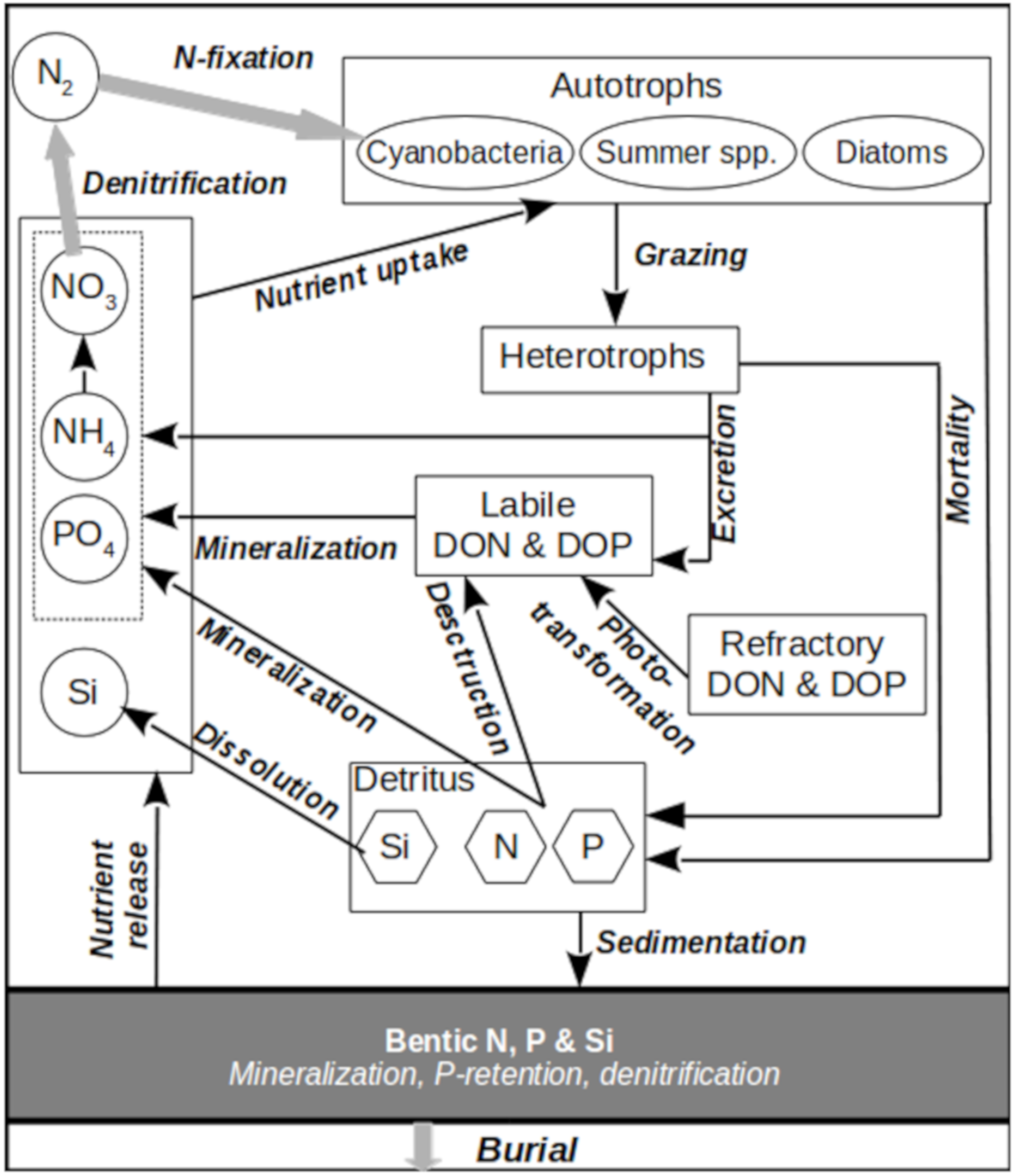
In the current version of SPBEM-2, the scheme of biogeochemical fluxes (Figure 1,

Table 2. Biogeochemical fluxes.

Flux	Definition	Units
PPi	Net primary production	mg N m−3 day−1
Mi	Mortality of autotroph	mg N m−3 day−1
Gi	Consumption of i-th autotroph group by heterotrophs	mg N m−3 day−1
Si	Sinking of autotrophs	mg N m−3 day−1
FNF,i=1	Nitrogen fixation	mg N m−3 day−1
KN(P)	Consumed food	mg N (P) m−3 day−1
EN	Excretion of ammonium by heterotrophs	mg N m−3 day−1
EP	Excretion of phosphate by heterotrophs	mg P m−3 day−1
MZ	Mortality of heterotrophs	mg N m−3 day−1
UN(P)(S)	Unassimilated food	mg N (P) (Si) m−3 day−1
WDN(P)	Destruction of detritus	mg N (P) m−3 day−1
GN(P)	Consumption of detritus by heterotrophs	mg N (P) m−3 day−1
SN(P)(S)	Sinking of detritus	mg N (P) (Si) m−3 day−1
WDS	Dissolution of silica	mg Si m−3 day−1
WDLN(P)	Mineralization of N- and P-dissolved organic labile fractions	mg N (P) m−3 day−1
VN	Ammonium uptake	mg N m−3 day−1
WO	Nitrification	mg N m−3 day−1
VO	Nitrate uptake	mg N m−3 day−1
WR	Pelagic denitrification	mg N m−3 day−1
VP	Phosphate uptake	mg P m−3 day−1
VS	Silica uptake	mg Si m−3 day−1
WDRN(P)	Phototransformation of N- and P-dissolved organic refractory fractions	mg N (P) m−3 day−1

), described by the biogeochemical translocation functions $\Phi$ (the “right-hand sides”), in a system of advection-diffusion equations is defined as follows:

$${\Phi }_{\mathrm{A}i}=P{P}_i-M_i-G_i-S_i\left(+F_{NF,i=1}\right)$$

(1)

$${\Phi }_{ZH}=K_N-E_N-M_Z$$

(2)

$${\Phi }_{DN}=M_H+U_N+{\displaystyle \sum }_{i=1}^3{M}_i-W_{DN}-G_N-S_N$$

(3)

$${\Phi }_{DP}=M_H/{\lambda }_{ZH}+U_P+{\displaystyle \sum }_{i=1}^3{M}_i/{\lambda }_{AN}-W_{DP}-G_P-S_P$$

(4)

$${\Phi }_{DS}=U_S+M_2/{\lambda }_{AS}-W_S-S_S$$

(5)

$${\Phi }_{NN}=\left(1-EDOM\right)\times E_N+W_{DLN}+\left(1-FDET\right)\times W_{DN}-V_N-W_O$$

(6)

$${\Phi }_{NO}=W_O-V_O-W_R$$

(7)

$${\Phi }_{NP}=\left(1-EDOM\right)\times E_P+W_{DLP}+\left(1-FDET\right)\times W_{DP}-V_P$$

(8)

$${\Phi }_{NS}=E_S-V_S$$

(9)

$${\Phi }_{LDON}=EDOM\times E_N-W_{DLN}+W_{DRN}+FDET\times W_{DN}$$

(10)

$${\Phi }_{LDOP}=EDOM\times E_P-W_{DLP}+W_{DRP}+FDET\times W_{DP}$$

(11)

$${\Phi }_{RDON}=-W_{DRN}$$

(12)

$${\Phi }_{RDOP}=-W_{DRP}$$

(13)

$$\begin{array}{ll}{\Phi }_{{\mathrm{O}}_2}=& {\mathsf{\beta }}_{\mathrm{PE}}{\displaystyle \sum }_{\mathrm{i}=1}^3{\mathrm{PP}}_{\mathrm{i}}\left(+F_{NF,i=1}\right)+{\mathsf{\beta }}_{\mathrm{WR}}{\mathrm{W}}_{\mathrm{R}}-{\mathsf{\beta }}_{\mathrm{WD}}{\mathrm{O}}_{\mathrm{BN}}\\ & -\left({\mathsf{\beta }}_{\mathrm{PE}}{\mathrm{E}}_{\mathrm{N}}+{\mathsf{\beta }}_{\mathrm{WD}}{\mathrm{W}}_{\mathrm{DN}}+{\mathsf{\beta }}_{\mathrm{WO}}{\mathrm{W}}_{\mathrm{O}}+{\mathsf{\beta }}_{\mathrm{WD}}{\mathrm{W}}_{\mathrm{DLN}}\right)\\ & \times \left(1.5+0.5\times tanh\left({\mathsf{\beta }}_{\mathrm{BOC}}-\frac{O_2}{{\mathsf{\beta }}_{\mathrm{SBOC}}}\right)\right)\end{array}$$

(14)

The equations for the sediment variables are written as:

$$\frac{\mathrm{dBN}}{\mathrm{dt}}={\displaystyle \sum }_{\mathrm{i}=1}^3{\mathrm{S}}_{\mathrm{i}}+S_N+{\mathrm{X}}_{\mathrm{N}}-{\mathrm{W}}_{\mathrm{BN}}-{\mathrm{B}}_{\mathrm{BN}}$$

(15)

$$\frac{\mathrm{dBP}}{\mathrm{dt}}={\displaystyle \sum }_{\mathrm{i}=1}^3{\mathrm{S}}_{\mathrm{i}}/\mathsf{\alpha }\mathrm{n}+S_P+{\mathrm{X}}_{\mathrm{P}}-{\mathrm{W}}_{\mathrm{BP}}-{\mathrm{B}}_{\mathrm{BP}}$$

(16)

$$\frac{dBS}{dt}=S_2+S_s-{\mathrm{W}}_{\mathrm{BS}}-{\mathrm{B}}_{\mathrm{BS}}$$

(17)

Most of the parameterizations implemented in Equations (1)–(9) and (14)–(17) were drawn from our previous publications, particularly from [6]. For the sake of the readers’ convenience, a full mathematical description of these formulations is repeated in Appendix A, together with new formulations for dissolved organic nutrients, where the initial forms of the formulations were taken from the carbon incarnation of BALTSEM (BALTSEM-C) [13]. Here, we discuss the assumptions behind the chosen definitions and interpret the newly introduced variables.

The new translocation functions (Equations (10)–(13)), describing biogeochemical transformations of the dissolved organic nitrogen (DON) and phosphorus (DOP), include the following sources and sinks described below. Since our original formulation [6,32,34] does not explicitly resolve diurnal processes, we do not account for dissolved organic substances whose lifetime is a day or less. We are also not interested in the geological scales of thousands of years. Therefore, only two fractions of DON and DOP were introduced into the modified SPBEM-2. The first fraction is considered to be “labile,” with a characteristic lifetime of about 1 year. The sources of labile organic matter are: inputs from land, part of the excretion of heterotrophs (E_N(P)), part of mineralized detritus (W_DN(P)), and influx due to the photochemical transformation of refractory organic matter (W_DRN(P)). A sink for labile organic matter is mineralization (W_DLN(P)) into dissolved inorganic nitrogen and phosphorus.

$$W_{DLN\left(P\right)}=a_{mN\left(P\right)}exp\left(b_{mN\left(P\right)}T\right)LDON\left(P\right)$$

(18)

where $a_{mN\left(P\right)}$ is mineralization rate and $b_{mN\left(P\right)}$ is a temperature constant (see

Table A3. Mineralization and apportionment of sediment fluxes.

Symbol	Parameters	Units	N	P	Si
$a_{dN\left(P\right)}$	Detritus destruction rate at 0 °C	day−1	0.02	0.02
$b_{dN\left(P\right)}$	Temperature constant for destruction	°C−1	0.15	0.15
$a_{mN\left(P\right)}$	Mineralization rate at 0 °C	day−1	0.004	0.004
$b_{mN\left(P\right)}$	Temperature constant for mineralization	°C−1	0.15	0.15
$a_{uv}$	Photo-transformation rate	day−1	0.0005	0.0005
${\epsilon }_{uv}$	Extinction constant of the ultraviolet radiation	m−2 W	0.02	0.02
$a_{wS}$	Dissolution rate of silica at 0 °C	day−1			0.002
$b_{wS}$	Temperature constant for dissolution	°C−1			0.1
$a_{bwN\left(P\right)\left(S\right)}$	Mineralization rate of sediment variables at 0 °C	day−1	0.0005	0.0005	0.0002
$b_{bwN\left(P\right)\left(S\right)}$	Temperature constant for sediment mineralization	°C−1	0.05	0.05	0.05

).

The second fraction includes all the remaining dissolved organic compounds considered “refractory,” and its transformation is determined only by the process of photochemical oxidation. In the present version of our model, we disregard the autochthonous production of refractory material considered, for instance, in the ERSEM model [36]. Thus, the only source of refractory organic nutrients here is that part of the land inputs which comes with the river runoff as humic substances and iron-humate complexes [37,38]. A small part of the refractory DON and DOP is transferred into a bioavailable labile form by the photochemical transformation (W_DRN(P)).

$$W_{DRN\left(P\right)}=a_{uv}exp\left({\epsilon }_{uv}{I}_z\right)RDON\left(P\right)$$

(19)

where $I_z$ is the photosynthetically active radiation on the z level (see Equation (A6)), $a_{uv}$ is a rate of photo-transformation, and ${\epsilon }_{uv}$ is a factor describing faster extinction of the ultraviolet radiation with depth (see Table A3).

As a result of this modification of the dissolved organic matter sub-model, the directions and interpretations of the biogeochemical fluxes have been changed, compared to [31]. In the presented version of SPBEM-2, part of the decomposed detritus is immediately mineralized to ammonium and phosphate, and part is hydrolyzed to a labile form of organic matter. Heterotroph excretion fluxes have also been revised. In the new version, some of the catabolic products are excreted in organic form and enter the pool of labile organic matter. However, we still disregard both the extracellular excretion (exudation) and possible utilization of DON and DOP by the phytoplankton.

Adding equations for the dissolved form of organic matter required a revision of the sedimentation and mineralization rates of detritus. Because in the previous model’s version (SPBEM), the variables of particulate nitrogen detritus and particulate phosphorus detritus were the only form of dead organic matter, its sedimentation rate was underestimated in comparison with the observed values in order to account for the DOM implicitly included in detritus variables. The introduction of dissolved organic nutrients made it possible to adjust the detritus sinking velocity closer to the reported ranges [23,39,40], increasing it, for example, from 2.6 to 6.6 m day⁻¹ (at 10 °C). These values may seem underestimated in comparison to the sinking velocities of diatom aggregates and fecal pellets of 50–100 m day⁻¹ [39], which, however, are considered to be a minor component of the total downward flux of the organic matter in the Baltic Sea [41]. Such an augmentation of the detritus removal from the surface layers required a significant intensification of the detritus destruction rate, from 0.004 to 0.088 day⁻¹ (at 10 °C). As a result, the nutrient retention capacity in the water column was maintained almost the same as in the comparably well-validated simulation in [31].

A full mathematical description of the parameterizations used in Equations (1)–(17), including all the coefficients and constants, is given in the Appendix A.

2.2. Data

The data used in this study originate mostly from the international database collected during the Gulf of Finland Year 2014 [42], which contains observations made by the Estonian, Finnish, and Russian scientific institutions and monitoring authorities for the period from 1999 to 2014. Data from occasional field surveys, conducted by other research vessels, were taken from the Baltic Environmental Database (BED, http://nest.su.se/bed). In total, data from over 4000 oceanographic stations were used. The average monthly values of river runoff and nutrient land loads were taken from the HELCOM Pollution Load Compilation database (HELCOM PLC-Water, http://nest.su.se/helcom_plc). The annual values were decomposed into monthly values using historical seasonal cycles, according to [32]. The separation into labile and refractory components was conducted in accordance with [31], assuming a 30% bioavailability of dissolved organic nitrogen and 80% bioavailability of dissolved organic phosphorus. The recent annual nitrogen atmospheric deposition was taken from [43] and decomposed into monthly values, as in [32].

2.3. Model Set-Up and Initial and Boundary Conditions

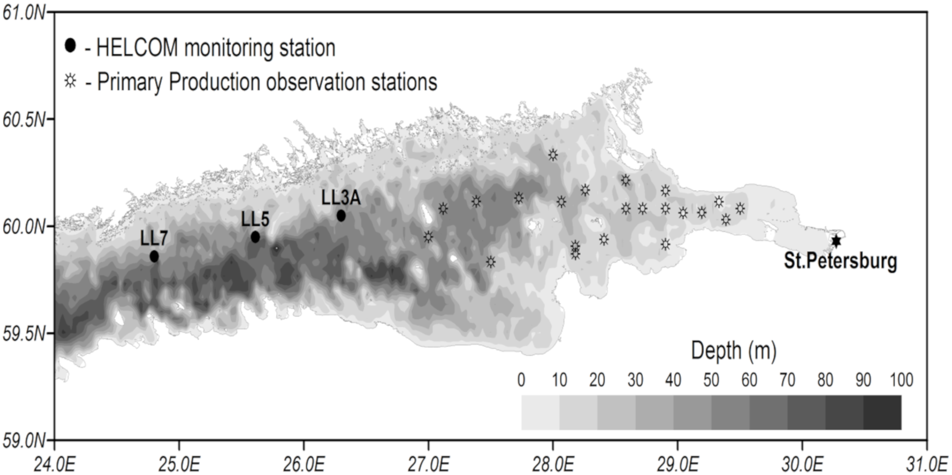
The computational grid covers the Gulf of Finland from Neva Bay to the meridian of 24.08° E, where the open boundary is located (Figure 2). The horizontal resolution of the spherical grid is 2′ in latitude and 4′ in longitude (~2 nautical miles), and the vertical resolution for the z-coordinate is 3 m from the surface to the bottom.

The initial fields of the temperature, salinity, and biogeochemical variables of the model were built from the observed vertical profiles of these oceanographic parameters, which were averaged for the winter months of 2002–2012 by interpolation into the nodes of the computational grid. The values of the sea level elevation and components of the current velocity were initially set equal to zero. The initial fields of benthic variables were taken from the final distributions, simulated from 2009 to 2014 using the previous version of SPBEM-2 and discussed in [31].

Both the initial conditions and conditions at the western boundary were obtained by processing the data from the international database [42] and BED. To resolve both the seasonal and interannual variations in the characteristics at the open boundary, the observed vertical profiles from the area between 23° E and 24.7° E longitude were step-wise horizontally averaged over successive 15-day time intervals. Subsequently, the averaged data were interpolated into a continuous time series. In this way, the boundary conditions were generated for the temperature, salinity, inorganic nitrogen, phosphorus, silicon, and organic matter. During the simulations, the boundary conditions for various forms of organic matter (two forms of dissolved organic nutrients, phytoplankton, and detritus) were determined as a fraction of the total organic amount, estimated from observations as the difference between the total amount of nitrogen and phosphorus and their inorganic forms. The further splitting of the organic nutrients between labile and refractory forms was made to be identical to their ratios, which were simulated in the inner grid cell nearest to the boundary.

Atmospheric forcing was set based on the ERA-Interim reanalysis fields (https://www.ecmwf.int). The model uses fields of pressure, wind speed components, air temperature, humidity, short-wave and long-wave incoming radiation, and precipitation.

Accounting for a water residence time in the Gulf of Finland of 2–3 years [32], both the pelagic and benthic fields were further adjusted during a spin-up run of three years, performed with the repeating boundary conditions for 2009. Numerical experiments were run for the period from 1 January 2009 to 31 December 2014.

2.4. Model Performance

We demonstrate the model performance by (a) validating it with a quantitative model–data comparison for several variables, and (b) verifying the internal consistency of SPBEM-2 and its capability to reproduce important feedback loops (“the vicious circle” [43]).

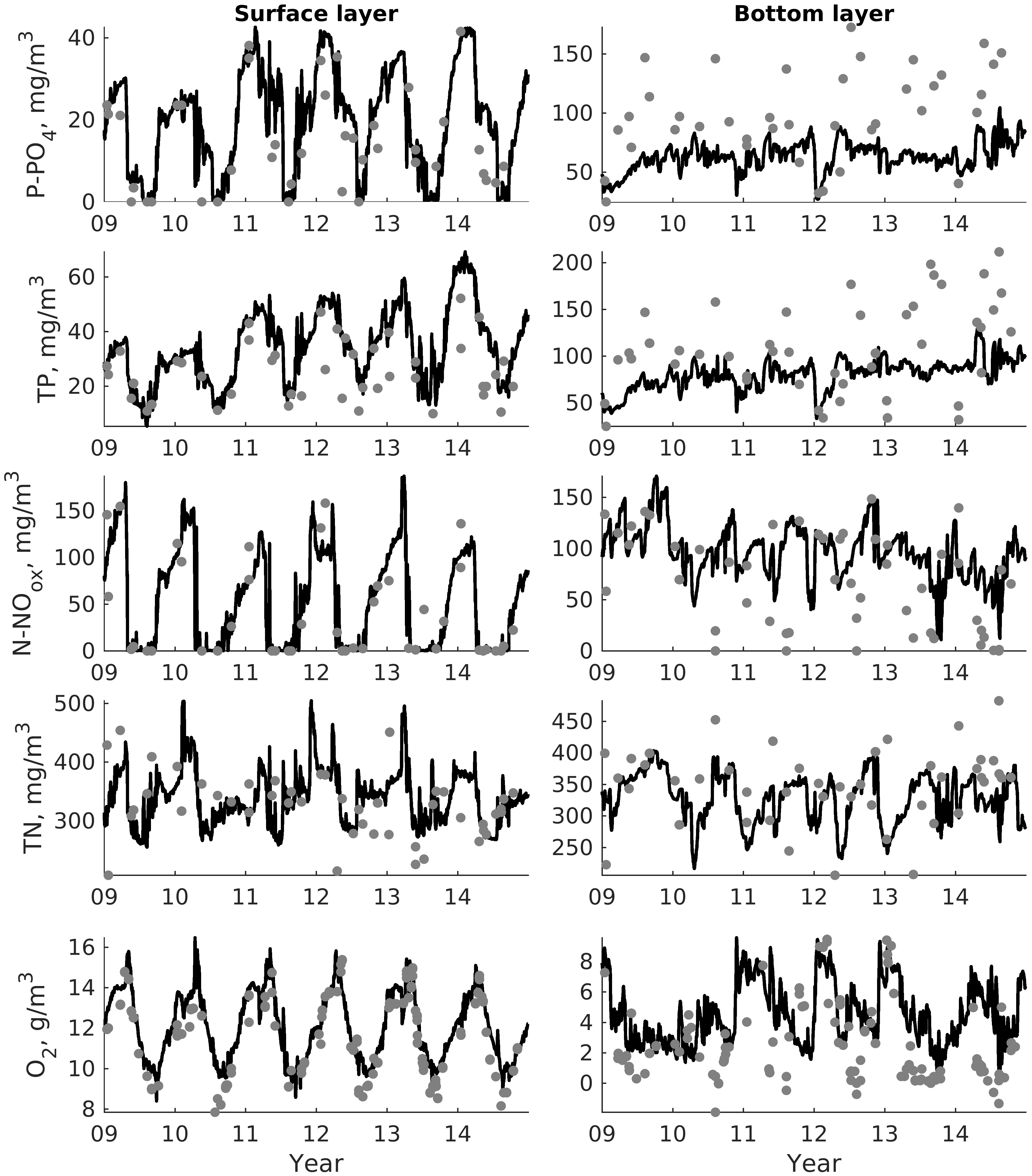
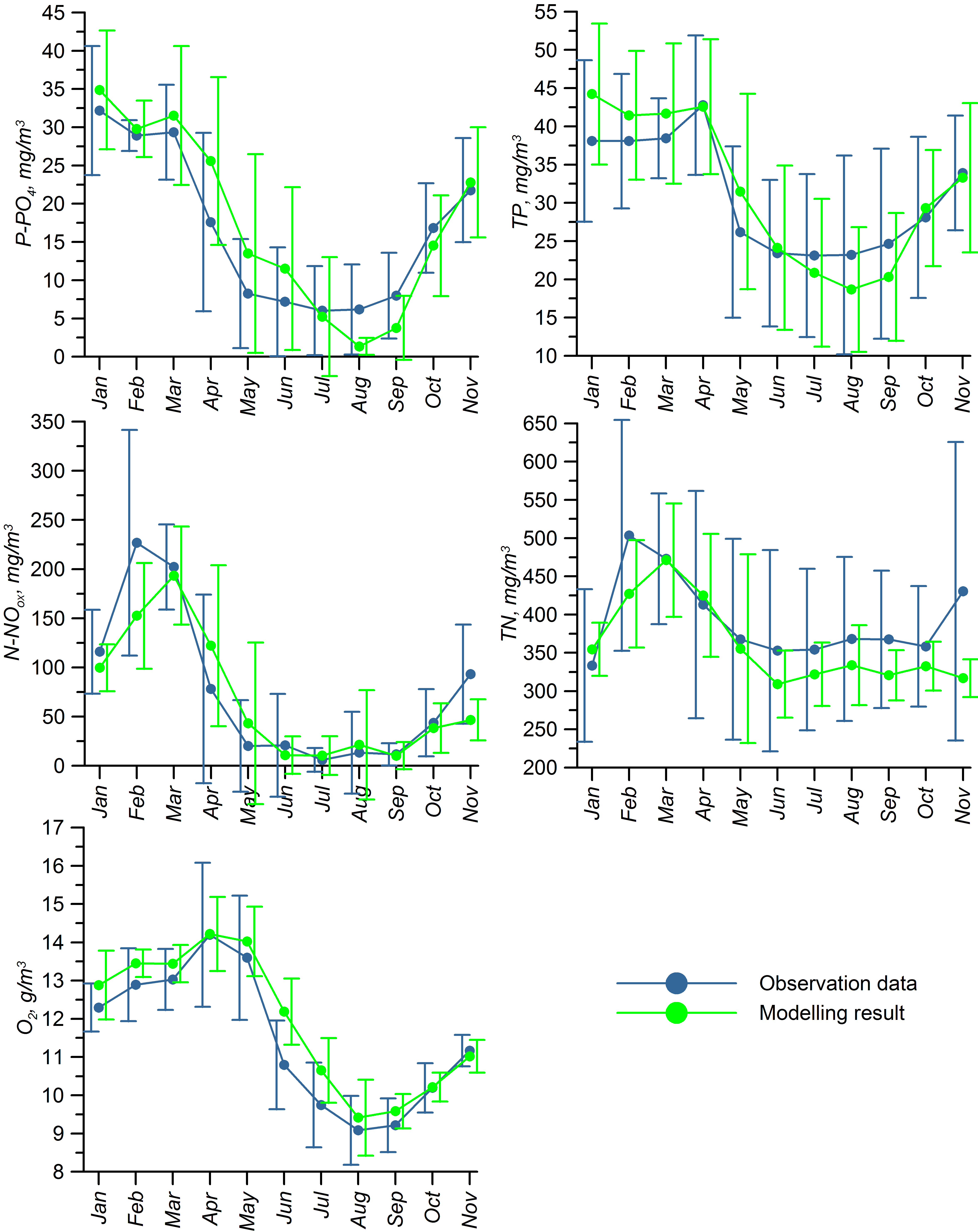
For validation, several methods of demonstrating the capabilities of SPBEM-2 were employed. A direct model–data comparison, with a seasonal and inter-annual resolution, was conducted for the most data-rich international monitoring stations, LL7, LL5, and LL3A (Figure 2). Considering that the real rugged bottom topography is approximated by a two-dimensional step function on a 2 × 2 nautical miles grid, a comparison with simulations was conducted as follows. First, we considered a 3 × 3 square of grid cells, where the central node was chosen as close to the average position of the monitoring station in question as possible. Further, we selected the cell, the depth of which was as close to the depth of the monitoring station as possible, and used the simulated profiles in this cell for comparison with the observed profiles. Unfortunately, all three stations with frequent monitoring are situated in the Western Gulf of Finland. Despite a large volume of observations in the Eastern Gulf of Finland, there are no intensive monitoring stations with an amount of measurements sufficient for making a seasonal to interannual model–data comparison, as described above for the western part of the gulf. Besides, a comparison at the sparse fixed stations gives less information about the quality of the simulation of the horizontal gradients in the distribution of ecosystem components. Therefore, we made a 3D statistical inter-comparison for the surface and bottom layers. For every single observation in the database, a corresponding daily averaged simulated variable was selected for the closest grid point as a match to this observation. The resulting pair-wise datasets were used for the calculation of some simple statistics. Apparently, with a grid size of 2 × 2 nautical miles, a grid cell height of 3 m, and daily averaging, we cannot expect a reproduction of the diurnal extremes in the observed variables, neither in these datasets, nor at the monitoring stations.

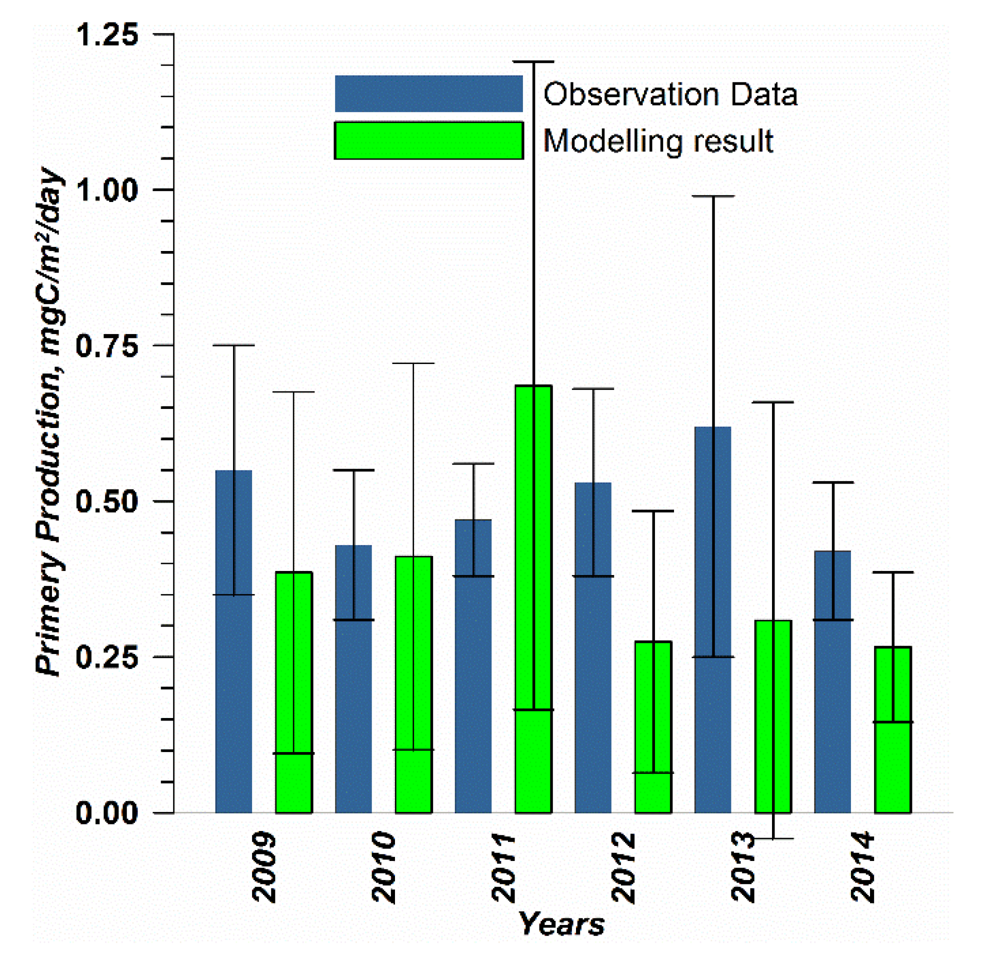
The capability of the model in simulating the biotic part of the ecosystem is demonstrated through a comparison with the measurements of phytoplankton primary production (PP) performed for years by the Russian State Hydrometeorological University in the Eastern Gulf of Finland. Measurements were carried out by the light–dark (or bulk) oxygen evolution method, which has been used for almost a century [44,45,46]. The method consists of the registration of changes in oxygen concentration using the high-precision Winkler method, with a 0.1% precision in oxygen determinations [47,48], following the 24 h incubation of natural communities in clear and dark bottles. The primary production is calculated as the sum of the rate of change in the oxygen concentration in clear bottles (equal to the primary production minus respiration) and that in dark bottles, i.e., the respiration. The measurements were conducted at a network of stations (Figure 2) from the end of July to the beginning of August. The selection of simulated values for comparison was conducted as follows. First, for every experimental estimate of PP, simulated values were compiled from a quadrate of 3 × 3 grid cells surrounding the station of measurements and for three days in a row, enveloping the time of measurements. Then, the simulated phytoplankton growth rates in nitrogen units, as well as the nitrogen fixation by cyanobacteria, were summed up and converted into carbon units, with a factor of 5.7. Finally, this dataset was averaged and used in a statistical model–data comparison for all the measurements in every simulated year. At the same time, we did not consider the routine chlorophyll observations as a good measure for comparison with the simulated phytoplankton biomass, expressed in nitrogen units, when such a comparison is conducted with quota coefficients that are fixed relative to carbon and chlorophyll [49,50]. A large intrinsic seasonal and interspecies variation in these quotas [51,52,53] makes this type of model–data comparison too uncertain and unconvincing [2].

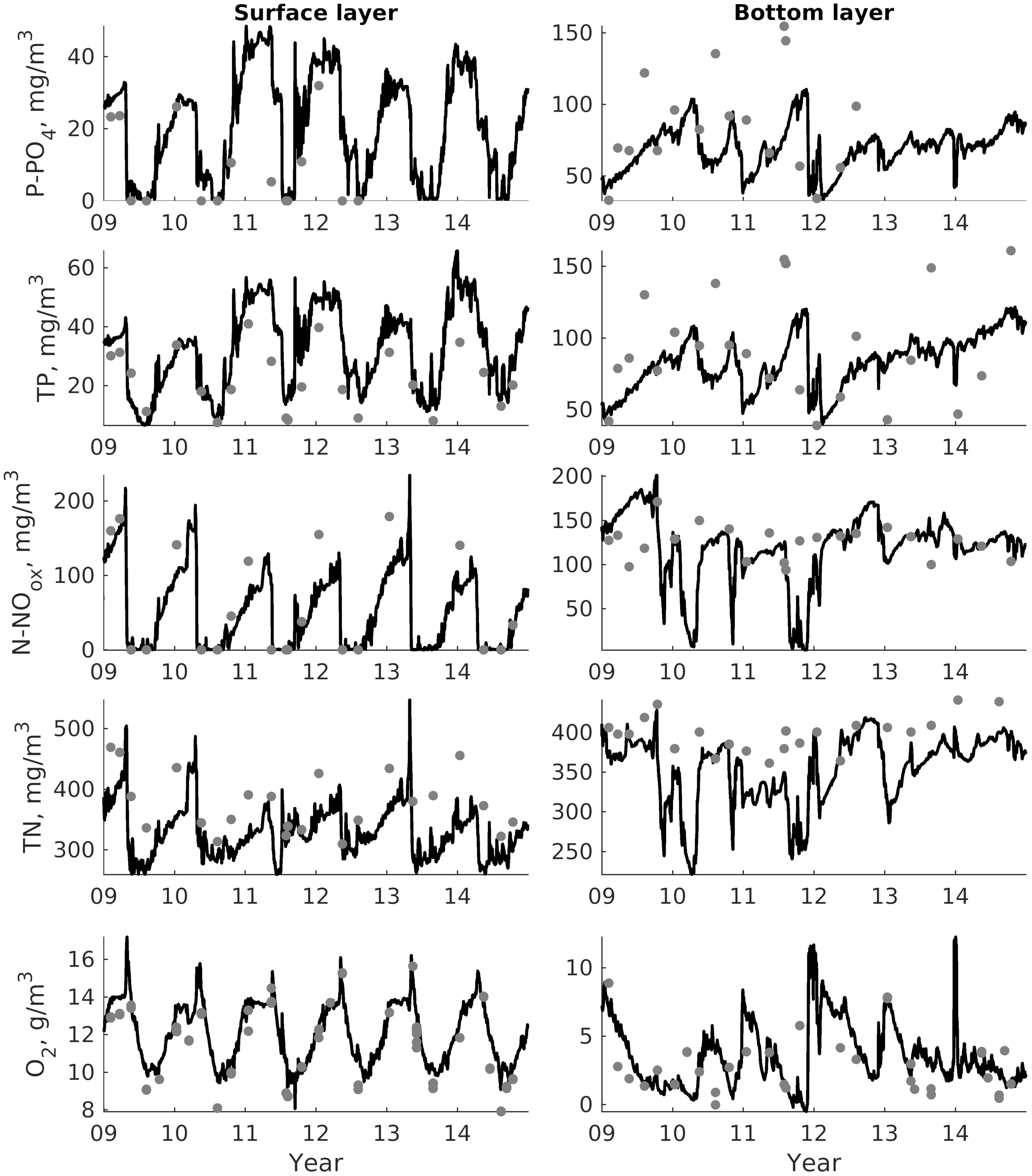
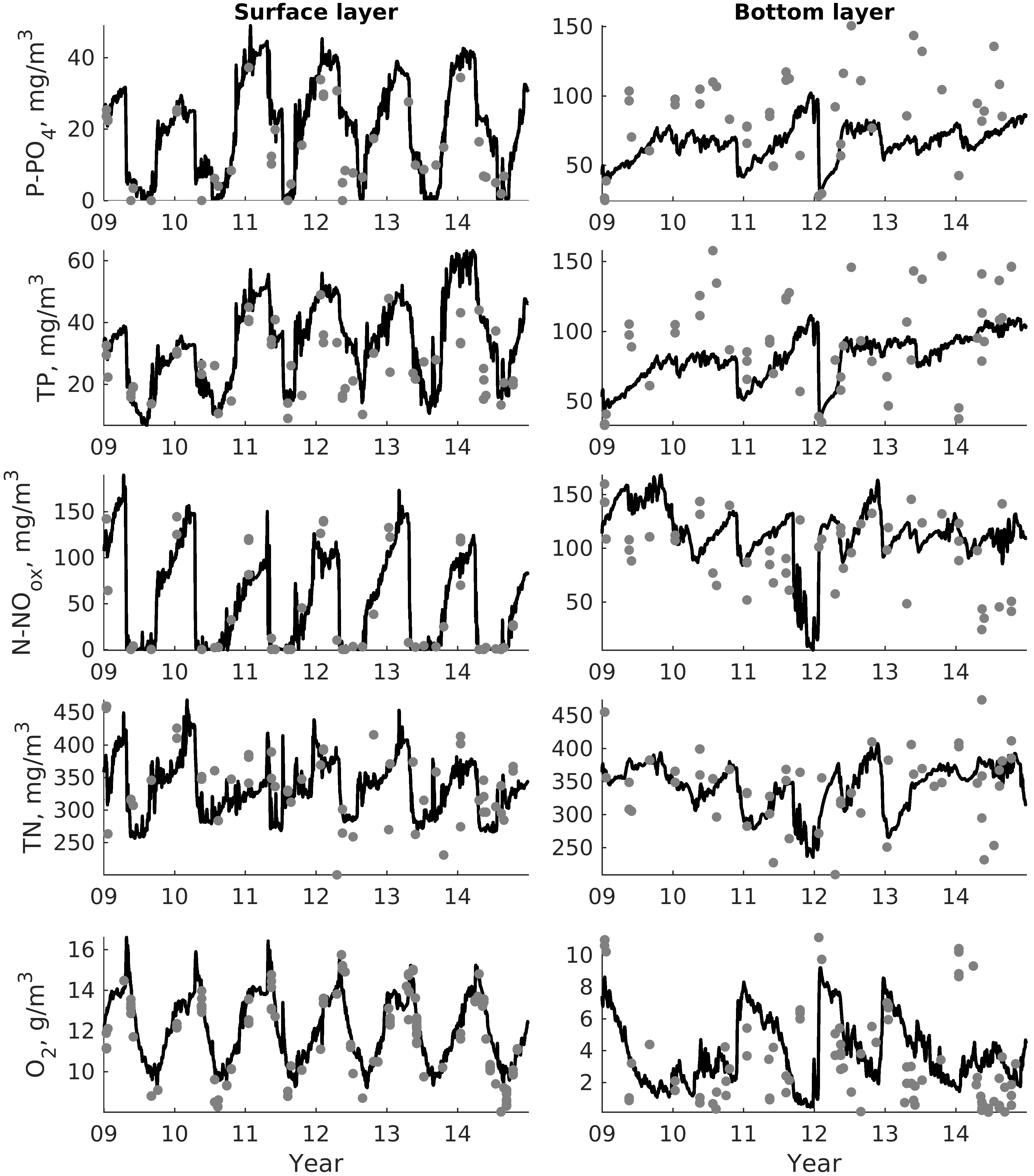
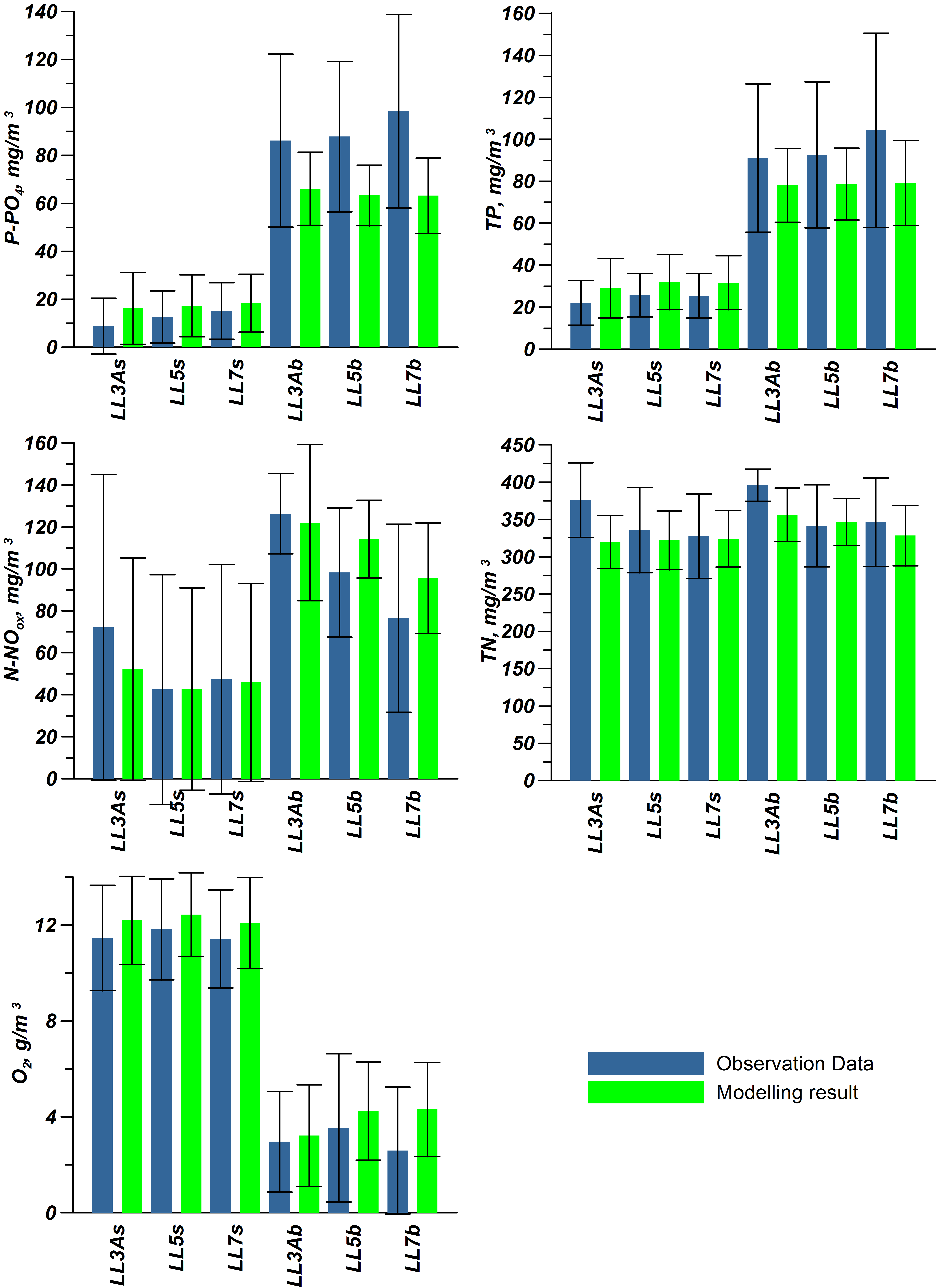
In addition to presenting compiled datasets as the usual graphs (Figure 3, Figure 4 and Figure 5), we used such simple statistics as the average, standard deviation, and coefficient of linear correlation, as well as more integral characteristics, such as the cost function (CF, Equation (18), [7]):

$$CF=\left|\frac{Mea{n}_{Mod}-Mea{n}_{Obs}}{ST{D}_{Obs}}\right|$$

(20)

where Mean_Mod and Mean_Obs are the averages of simulated and observed variables, respectively, and STD_Obs is the standard deviation of observed variables.

3. Results and Discussion

As shown in [31], the hydrodynamic module of SPBEM-2 rather plausibly reproduces the thermohaline characteristics and water dynamics of the Gulf of Finland at the simulated seasonal and interannual scales. Therefore, this study focused solely on a validation and verification of the biogeochemical part.

3.1. Validation

As demonstrated in Figure 3, Figure 4, Figure 5 and Figure 6 and

Table A4. Statistical comparison of the simulation results with the observational data at intensive monitoring stations.

Variable	Mean		Std		Statistics
	Obs	Model	Obs	Model	R	CF	N
	Station LL3A
	Surface Layer
Np	8.8	16.2	11.6	15.0	0.70	0.64	15
TotP	22.1	29.0	10.6	14.1	0.83	0.66	38
No	72.1	52.2	72.8	53.1	0.89	0.27	28
TotN	375.9	320.0	49.9	35.5	0.72	1.12	38
O2	11.5	12.2	2.2	1.8	0.96	0.33	163
	Bottom Layer
Np	86.1	66.1	36.1	15.2	0.37	0.56	17
TotP	91.1	78.1	35.3	17.6	0.35	0.37	39
No	126.3	122.0	19.1	37.2	0.03	0.22	37
TotN	395.9	356.4	21.5	35.9	0.41	1.84	38
O2	3.0	3.2	2.1	2.1	0.52	0.12	48
	Station LL5
	Surface Layer
Np	12.6	17.3	10.9	12.9	0.82	0.43	53
TotP	25.7	32.0	10.4	13.1	0.67	0.61	74
No	42.5	42.7	54.7	48.2	0.84	0.00	67
TotN	335.8	322.0	57.2	39.3	0.38	0.24	72
O2	11.8	12.4	2.1	1.7	0.92	0.29	256
	Bottom Layer
Np	87.8	63.3	31.4	12.6	0.57	0.78	53
TotP	92.6	78.7	34.8	17.1	0.46	0.40	72
No	98.3	114.2	30.8	18.5	0.06	0.52	70
TotN	341.6	346.9	55.0	31.4	0.23	0.10	70
O2	3.5	4.2	3.1	2.0	0.31	0.23	105
	Station LL7
	Surface Layer
Np	15.1	18.4	11.8	12.0	0.78	0.28	48
TotP	25.4	31.6	10.7	12.8	0.69	0.58	68
No	47.4	45.9	54.7	47.2	0.91	0.03	61
TotN	327.6	324.2	56.6	37.7	0.16	0.06	69
O2	11.4	12.1	2.0	1.9	0.95	0.33	363
	Bottom Layer
Np	98.4	63.2	40.4	15.7	0.58	0.87	47
TotP	104.3	79.2	46.3	20.3	0.44	0.54	69
No	76.5	95.6	44.8	26.3	0.43	0.43	72
TotN	346.4	328.5	59.2	40.5	0.16	0.30	67
O2	2.6	4.3	2.6	2.0	0.49	0.65	148

, SPBEM-2 quite realistically reproduces the nutrient and oxygen dynamics in the surface layer. The lowest values of the coefficients of the linear correlation in the surface layer were found for the total nitrogen (TN) at the LL5 and LL7 stations, which were 0.38 and 0.16, respectively. At the same time, the model–data differences in the overall averages of TN did not exceed a few percent, while the difference in standard deviations was much smaller than the standard deviation of the observations (Table A4). As seen in Figure 5 and Figure 6, the low values of the correlation coefficients can be explained by some biases between the simulated and observed timing of extremes. Such biases could have a different origin, including analytical problems with the measurements of the total nitrogen [54] and inaccuracies in the prescribed boundary conditions, both in the land loads and at the open boundary. However, these differences do not significantly affect the general conclusion concerning the plausibility of the model performance. The usefulness of combining the usual graphical presentation and simple statistical estimates for the analysis of the model’s skill should also be noted.

On the other hand, the highest correlation coefficients belonged to a comparison of oxidized forms of nitrogen (NO) in the surface layer at LL3A and LL7, reaching values of 0.8 and 0.9, respectively. The differences in the mean values and standard deviations varied from rather insignificant at LL3A to almost non-existent at LL5 and LL7 (Figure 6; Table A4). The graphical comparison allows for a further refinement of such a conclusion, with respect both to the timing and concentration of the winter nutrient maxima (Figure 3, Figure 4 and Figure 5).

In the bottom layers, the results of the model–data comparison were mostly determined by the overestimated oxygen concentrations in the model (Figure 6, see also [31]), especially during the summer minima. The discrepancy increased with the depth of the compared monitoring stations (cf. Figure 3, Figure 4 and Figure 5), reaching, on average, 1.7 mg O₂ L⁻¹ at LL7. Additionally, in the model, the hypoxic conditions (O₂ < 2.86 mg O₂L⁻¹) were found less frequently than in observations. One of the evident reasons for such a general deviation is that the smoothed model bottom is shallower than the depth of the monitoring stations that, once upon a time, had been intentionally chosen to represent the deepest point in the area. For instance, at LL7, we compare measurements from samples taken at 80–90 m horizons to simulated concentrations from the model bottom layer at 73.5 m, and such a depth difference is important within the marked vertical gradients of the oxygen concentration (see also integral model–data comparison in Section 3.2). Another possible reason could also be a larger retention of nutrients in the surface layer, with a lesser detritus transport to the deep sediments and, correspondingly, a reduced biochemical oxygen demand (BOD). However, for the time being, we have postponed a corresponding enquiry and refining until a further model development, particularly of its sediment module, has been achieved.

Generally, the maximal discrepancies, both graphical and statistical, were found in a comparison of the deep layer phosphates and, consequently, the total phosphorus dynamics (Figure 3, Figure 4, Figure 5 and Figure 6; Table A4). The simulated concentrations in the bottom layer are systematically underestimated. This underestimation is a direct consequence of the underestimated flux from the bottom, which, in accordance with our parameterization (A61–A63), is substantially reduced because of the overestimated oxygen concentration. On the contrary, the simulated dynamics of the NO variable did measure up to observation substantially better, even despite some mismatch in the extrema, formally indicated by the practically non-existent linear correlation between the simulated variables and observations (Table A4), particularly at LL3A and LL5. Additionally, an overestimation of the mean values of NO at the deeper stations, LL5 and, especially, LL7, might indicate a somewhat underestimated rate of denitrification as a result of the overestimated availability of oxygen for the oxidation of organic matter.

The assessment of the model capability to reproduce the seasonal spatial-temporal dynamics, in general, for the entire Gulf of Finland was made by comparing six-year monthly averages and standard deviations of all the available measurements and, corresponding to them, simulated values extracted and compiled from 3D fields, as explained in Section 2.4. The results of this model–data comparison are presented in Figure 7 for the surface layer. For the bottom layer (Figure 8), we used only oceanographic stations deeper than 20 m, that is, deeper than the average depth of the seasonal thermocline in order to prevent the inclusion of the waters occurring within the seasonal mixed layer into the comparison. December is excluded from this comparison because only two oceanographic stations were available for this month during the entire period of 2009–2014.

These comparisons further confirm the main conclusion that could be made from an analysis of the monitoring stations: so far, the SPBEM-2 better reproduces the nutrient and oxygen dynamics in the surface layers (Figure 7) compared to the deep layers (Figure 8). Most discrepancies occurring between the measured and simulated inorganic nutrient concentrations were almost quantitatively equal to those discrepancies found for the total nitrogen and phosphorus concentrations, which indicates a very good reproducibility of the organic nutrient concentrations. In the surface layer, both the winter maxima and summer minima values are quite realistic. However, the noticeable discrepancies between the observation and simulation for inorganic phosphorus and nitrogen in April and May indicate a delayed phytoplankton spring bloom in the model. In the deep layers, the overestimated oxygen concentration results in under and overestimated concentrations of phosphate and inorganic oxidized nitrogen, respectively.

3.2. Verification

To demonstrate the causal relationships between oxygen availability and nutrient redox alterations, we extracted and presented both simulation and observation results as time–depth contour plots, built on all the vertical profiles horizontally averaged over the entire modeled domain (Figure 2 and Figure 9, cf. also Figure 2 in [55]). Among the other expected patterns of the hypothetical “vicious circle of the Baltic Sea eutrophication” [43,54,56], the expansion of the long-lasting oxygen deficit and hypoxia in 2009–2010, which extended over rather shallow and voluminous areas and were interrupted by the intensive vertical mixing in winter 2011, looks especially conspicuous. The mixing brought up phosphate reserves accumulated in the oxygen-deficient areas, thus increasing the winter surface DIP concentrations far above the average values (see also Figure 3, Figure 4 and Figure 5), while the DIN concentration remained at a more typical level. As a result, the winter (March) DIN:DIP ratio dropped to rather low values, with corresponding consequences for the expansion and dynamics of both the nitrogen limitation and nitrogen fixation by cyanobacteria (Figure 10) and, consequently, for the phytoplankton primary production (Figure 11,

Table 3. Comparison of the simulated primary production (g C m⁻² day⁻¹) with estimates obtained using the bulk light–dark oxygen method at the end of July until the beginning of August in the Eastern Gulf of Finland (positions of the stations with measurements are indicated in Figure 2).

	Primary Production, g C m−2 day−1
	Model		Observations
Year	Mean	Std	Mean	Std	N
2009	0.39	0.29	0.55	0.20	17
2010	0.41	0.31	0.43	0.12	12
2011	0.69	0.52	0.47	0.09	10
2012	0.27	0.21	0.53	0.15	9
2013	0.31	0.35	0.62	0.37	12
2014	0.27	0.12	0.42	0.11	15
Mean	0.39	0.39	0.50	0.21

).

As is well known, from an analysis of both observations [57,58,59,60,61,62] and simulations [33,34,63], and as demonstrated in Figure 10A and Figure 12, the phosphorus limitation in Neva Bay and some other estuaries is gradually replaced by the nitrogen limitation offshore. This knowledge and these modelling results make questionable the conclusion concerning the present-day nitrogen limitation of these areas and the emergence of a phosphorus limitation only in the distant future (cf. Figure 6 in [64]). However, such an average distribution can be substantially altered by the nutrient exchange with the Northern Baltic Proper [55] and internal biogeochemical interactions. Similar to the succession of events in 1995–1997 [65,66], the extensive hypoxia of 2009–2010 resulted in an expansion of the nitrogen-limited surface waters, with very elevated stocks of the winter Redfield excess of inorganic phosphorus (calculated in weight units as eDIP = DIP – DIN/7; see e.g., [54] and references therein) in 2011 (Figure 10B, right). Consequently, the simulated rate of nitrogen fixation by cyanobacteria in 2011 increased many-fold, while the area of elevated rates substantially expanded (Figure 10C). It should also be noted that the larger-than-usual expansion of cyanobacteria accumulations over the Gulf of Finland in 2011, compared to 1979–2014 summer distributions, is unequivocally found also in the multi-decadal time-series of the satellite-detected accumulations of cyanobacteria [67].

This massive contribution of cyanobacteria to the phytoplankton primary production in 2011 is also quite clearly seen in comparison with the field estimates (Figure 11, Table 3). Even in the Eastern Gulf of Finland, where the nitrogen fixation rates were lower than in the rest of the Gulf of Finland (Figure 10C), the simulated primary production was almost two-fold higher than the one estimated by the light–dark oxygen evolution method. Most likely, the measured primary production is underestimated because the filamentous cyanobacteria could hardly be caught in the incubation bottles adequately. On the other hand, in other years, the simulated phytoplankton primary production was expected to be somewhat smaller than the measured production because the phytoplankton growth rate, simulated in nitrogen units, is by definition equal to the net primary production, while all the measurements represent some values intermediate between the gross and net primary production [68].

Considering the results of the validation and verification in general, it already appears that the presented version of SPBEM-2 is capable of plausibly reproducing all the major large-scale features and phenomena of the nutrient dynamics in the Gulf of Finland, especially in its surface productive layer that, for hypsographic reasons, contain and transform the major pools of nutrients. The expansion of SPBEM-2 with dissolved organic nutrients allows for a full account of the land loads in both historical and scenario simulations, thus reducing the uncertainty in forcing.

4. Conclusions

• A modified version of the coupled 3D hydrodynamical-biogeochemical St. Petersburg Eutrophication Model (SPBEM-2) has been presented, including a full description of the biogeochemical module, with all the equations and coefficients.
• The SPBEM-2 has been expanded with four new variables (the labile and refractory fractions of the dissolved organic nitrogen and phosphorus) and a redefinition of the detritus variables, allowing for a full account of the total amounts of nutrients as they are reported in field measurements and presented in environmental documents, thus alleviating one of the important sources of uncertainty in the boundary conditions.
• An extensive model–data comparison of the model performance in the Gulf of Finland from 2009 to 2014, based on over 4000 oceanographic stations, was conducted, showing that SPBEM-2 is capable of plausibly reproducing all the major large-scale features and phenomena of the seasonal and interannual nutrient dynamics in the Gulf of Finland, especially in its surface productive layer.
• Validation and verification of the capabilities of SPBEM-2 were conducted, showing the model to be a useful instrument in studies of the biogeochemical interactions determining the state of eutrophication and a necessary tool in both historical and scenario simulations.
• From the results and experience obtained from the performed model–data comparison, it was shown that it is very important to combine both formal (statistical) and expert (graphical) means of comparison in order to properly reveal and explain both the realistic model behavior and its deficiencies.

References

1. Meier, H.E.M.; Edman, M.; Eilola, K.; Placke, M.; Neumann, T.; Andersson, H.C.; Brunnabend, S.-E.; Dieterich, C.; Frauen, C.; Friedland, R.; et al. Assessment of Uncertainties in Scenario Simulations of Biogeochemical Cycles in the Baltic Sea. Front. Mar. Sci. 2019, 6, 46. [Google Scholar] [CrossRef] [Green Version]
2. Meier, H.E.M.; Edman, M.K.; Eilola, K.J.; Placke, M.; Neumann, T.; Andersson, H.C.; Brunnabend, S.-E.; Dieterich, C.; Frauen, C.; Friedland, R.; et al. Assessment of Eutrophication Abatement Scenarios for the Baltic Sea by Multi-Model Ensemble Simulations. Front. Mar. Sci. 2018, 5, 440. [Google Scholar] [CrossRef]
3. Ayzatulllin, T.A.; Leonov, A.V. Kinetika I mekhanizm okislitelnoi transformatsi I soedineniy rastvoryonnoy sery v morskoi vode (Kinetics and mechanism of the oxidizing transformation of reduced sulfur compounds in the sea water). Oceanology 1975, 15, 1026–1033. (In Russian) [Google Scholar]
4. Yakushev, E.V.; Mikhailovsky, G.E. Mathematical modelling of the influence of marine biota on the carbon dioxide ocean-atmosphere exchange in high latitudes. In Air-Water Gas Transfer; AEON Verlag & Studio: Hanau, Germany, 1995; pp. 37–48. [Google Scholar]
5. Yakushev, E.; Pollehne, F.; Jost, G.; Kuznetsov, I.; Schneider, B.; Umlauf, L. Analysis of the water column oxic/anoxic interface in the Black and Baltic seas with a numerical model. Mar. Chem. 2007, 107, 388–410. [Google Scholar] [CrossRef]
6. Savchuk, O.P. Nutrient biogeochemical cycles in the Gulf of Riga: Scaling up field studies with a mathematical model. J. Mar. Syst. 2002, 32, 253–280. [Google Scholar] [CrossRef]
7. Eilola, K.; Gustafsson, B.G.; Kuznetsov, I.; Meier, H.E.M.; Neumann, T.; Savchuk, O.P. Evaluation of biogeochemical cycles in an ensemble of three state-of-the-art numerical models of the Baltic Sea. J. Mar. Syst. 2011, 88, 267–284. [Google Scholar] [CrossRef]
8. Keller, D.P.; Hood, R.R. Comparative simulations of dissolved organic matter cycling in idealized oceanic, coastal, and estuarine surface waters. J. Mar. Syst. 2013, 109–110, 109–128. [Google Scholar] [CrossRef]
9. Isaev, A.V.; Eremina, T.R.; Ryabchenko, V.A.; Savchuk, O.P. Model estimates of the impact of bioirrigation activity of Marenzelleria spp. on the Gulf of Finland ecosystem in a changing climate. J. Mar. Syst. 2017, 171, 81–88. [Google Scholar] [CrossRef]
10. Aarnos, H.; Ylöstalo, P.; Vähätalo, A.V. Seasonal phototransformation of dissolved organic matter to ammonium, dissolved inorganic carbon, and labile substrates supporting bacterial biomass across the Baltic Sea. J. Geophys. Res. Biogeo. 2012, 117. [Google Scholar] [CrossRef]
11. Vichi, M.; May, W.; Navarra, A. Response of a complex ecosystem model of the northern Adriatic Sea to a regional climate change scenario. Clim. Res. 2003, 24, 141–159. [Google Scholar] [CrossRef]
12. Daewel, U.; Schrum, C. Simulating long-term dynamics of the coupled North Sea and Baltic Sea ecosystem with ECOSMO II: Model description and validation. J. Mar. Syst. 2013, 119–120, 30–49. [Google Scholar] [CrossRef]
13. Gustafsson, E.; Deutsch, B.; Gustafsson, B.G.; Humborg, C.; Mörth, C.-M. Carbon cycling in the Baltic Sea—The fate of allochthonous organic carbon and its impact on air-sea CO2 exchange. J. Mar. Syst. 2014, 129, 289–302. [Google Scholar] [CrossRef]
14. Große, F.; Fennel, K.; Laurent, A. Quantifying the Relative Importance of Riverine and Open-Ocean Nitrogen Sources for Hypoxia Formation in the Northern Gulf of Mexico. J. Geophys. Res. Oceans 2019, 124, 5451–5467. [Google Scholar] [CrossRef]
15. Flato, G.M. Earth system models: An overview: Earth system models. WIREs Clim. Change 2011, 2, 783–800. [Google Scholar] [CrossRef]
16. Patara, L.; Visbeck, M.; Masina, S.; Krahmann, G.; Vichi, M. Marine biogeochemical responses to the North Atlantic Oscillation in a coupled climate model. J. Geophys. Res. 2011, 116. [Google Scholar] [CrossRef] [Green Version]
17. Patara, L.; Vichi, M.; Masina, S. Impacts of natural and anthropogenic climate variations on North Pacific plankton in an Earth System Model. Ecol. Model. 2012, 244, 132–147. [Google Scholar] [CrossRef]
18. Dutkiewicz, S.; Hickman, A.E.; Jahn, O.; Gregg, W.W.; Mouw, C.B.; Follows, M.J. Capturing optically important constituents and properties in a marine biogeochemical and ecosystem model. Biogeosciences 2015, 12, 4447–4481. [Google Scholar] [CrossRef] [Green Version]
19. Kriest, I. Calibration of a simple and a complex model of global marine biogeochemistry. Biogeosciences 2017, 14, 4965–4984. [Google Scholar] [CrossRef] [Green Version]
20. Kemena, T.P.; Landolfi, A.; Oschlies, A.; Wallmann, K.; Dale, A.W. Ocean phosphorus inventory: Large uncertainties in future projections on millennial timescales and their consequences for ocean deoxygenation. Earth Syst. Dynam. 2019, 10, 539–553. [Google Scholar] [CrossRef] [Green Version]
21. Sauerland, V.; Kriest, I.; Oschlies, A.; Srivastav, A. Multiobjective Calibration of a Global Biogeochemical Ocean Model Against Nutrients, Oxygen, and Oxygen Minimum Zones. J. Adv. Model. Earth Syst. 2019, 11, 1285–1308. [Google Scholar] [CrossRef]
22. Jassby, A.D.; Platt, T. Mathematical formulation of the relationship between photosynthesis and light for phytoplankton: Photosynthesis-light equation. Limnol. Oceanogr. 1976, 21, 540–547. [Google Scholar] [CrossRef] [Green Version]
23. Sergeev, Y.N.; Kolodochka, A.A.; Krummel, H.-D.; Kulesh, V.P.; Savchuk, O.P. Modelling of the Transport and Transformation Processes in the Sea; Leningrad Univ. Publ. House: Leningrad, Russia, 1979; p. 292. (In Russian) [Google Scholar]
24. Tian, R.C. Toward standard parameterizations in marine biological modeling. Ecol. Model. 2006, 193, 363–386. [Google Scholar] [CrossRef]
25. Dittmar, T.; Stubbins, A. Dissolved Organic Matter in Aquatic Systems. In Treatise on Geochemistry; Elsevier: Amsterdam, The Netherlands, 2014; pp. 125–156. [Google Scholar]
26. Karl, D.M.; Björkman, K.M. Dynamics of Dissolved Organic Phosphorus. In Biogeochemistry of Marine Dissolved Organic Matter; Elsevier: Amsterdam, The Netherlands, 2015; pp. 233–334. [Google Scholar]
27. Hansell, D.A. Recalcitrant Dissolved Organic Carbon Fractions. Annu. Rev. Mar. Sci. 2013, 5, 421–445. [Google Scholar] [CrossRef] [PubMed]
28. Schneider, B.; Dellwig, O.; Kuliński, K.; Omstedt, A.; Pollehne, F.; Rehder, G.; Savchuk, O. Biogeochemical cycles. In Biological Oceanography of the Baltic Sea; Snoeijs-Leijonmalm, P., Schubert, H., Radziejewska, T., Eds.; Springer: Dordrecht, The Netherlands, 2017; pp. 87–122. [Google Scholar]
29. Sipler, R.E.; Bronk, D.A. Dynamics of Dissolved Organic Nitrogen. In Biogeochemistry of Marine Dissolved Organic Matter; Elsevier: Amsterdam, The Netherlands, 2015; pp. 127–232. [Google Scholar]
30. Doval, M.D.; Fraga, F.; Pérez, F.F. Determination of dissolved organic nitrogen in seawater using Kjeldahl digestion after inorganic nitrogen removal. Oceanol. Acta 1997, 20, 713–720. [Google Scholar]
31. Vladimirova, O.; Eremina, T.; Isaev, A.; Ryabchenko, V.; Savchuk, O. Modelling Dissolved Organic Nutrients in the Gulf of Finland. Fundam. Prikl. Gidrofiz. 2019, 11, 90–101. [Google Scholar]
32. Savchuk, O.P.; Gustafsson, B.G.; Mueller-Karulis, B. BALTSEM a Marine Model for Decision Support within the Baltic Sea Region; Tech. Rep. 7; Baltic Nest Institute, Stockholm University: Stockholm, Sweden, 2012. [Google Scholar]
33. Neelov, I.A.; Isaev, A.V.; Ryabchenko, V.A.; Savchuk, O.P.; Vankevich, R.E. A simulation of the Gulf of Finland ecosystem with a 3-D model. In Proceedings of the Estonian Academy of Sciences. Biology. Ecology; Estonian Academy of Sciences: Tallinn, Estonia, 2003; Volume 52, pp. 346–359. [Google Scholar]
34. Savchuk, O.P.; Wulff, F. Long-term modeling of large-scale nutrient cycles in the entire Baltic Sea. Hydrobiologia 2009, 629, 209–224. [Google Scholar] [CrossRef]
35. Ryabchenko, V.A.; Karlin, L.N.; Isaev, A.V.; Vankevich, R.E.; Eremina, T.R.; Molchanov, M.S.; Savchuk, O.P. Model estimates of the eutrophication of the Baltic Sea in the contemporary and future climate. Oceanology 2016, 56, 36–45. [Google Scholar] [CrossRef]
36. Butenschön, M.; Clark, J.; Aldridge, J.N.; Allen, J.I.; Artioli, Y.; Blackford, J.; Bruggeman, J.; Cazenave, P.; Ciavatta, S.; Kay, S.; et al. ERSEM 15.06: A generic model for marine biogeochemistry and the ecosystem dynamics of the lower trophic levels. Geosci. Model Dev. Discuss. 2015, 8, 7063–7187. [Google Scholar] [CrossRef] [Green Version]
37. Kallianou, C.S.; Yassoglou, N.J. Bonding and oxidation state of iron in humic complexes extracted from some Greek soils. Geoderma 1985, 35, 209–221. [Google Scholar] [CrossRef]
38. Yang, R.; Su, H.; Qu, S.; Wang, X. Capacity of humic substances to complex with iron at different salinities in the Yangtze River estuary and East China Sea. Sci. Rep. 2017, 7, 1381. [Google Scholar] [CrossRef]
39. Sarthou, G.; Timmermans, K.R.; Blain, S.; Tréguer, P. Growth physiology and fate of diatoms in the ocean: A review. J. Sea Res. 2005, 53, 25–42. [Google Scholar] [CrossRef]
40. Bach, L.T.; Riebesell, U.; Sett, S.; Febiri, S.; Rzepka, P.; Schulz, K.G. An approach for particle sinking velocity measurements in the 3–400 μm size range and considerations on the effect of temperature on sinking rates. Mar. Biol. 2012, 159, 1853–1864. [Google Scholar] [CrossRef] [PubMed]
41. Blomqvist, S.; Heiskanen, A.-S. The challenge of sedimentation in the Baltic Sea. In A Systems Analysis of the Baltic Sea; Wulff, F., Rahm, L., Larsson, P., Eds.; Springer-Verlag: Berlin, Germany, 2001; pp. 211–227. [Google Scholar]
42. The Gulf of Finland Assessment. Reports of the Finnish Environment Institute; Raateoja, M., Setälä, O., Eds.; Finnish Environment Institute: Helsinki, Finland, 2016; Volume 27, p. 363. [Google Scholar]
43. Vahtera, E.; Conley, D.J.; Gustafsson, B.G.; Kuosa, H.; Pitkänen, H.; Savchuk, O.P.; Tamminen, T.; Viitasalo, M.; Voss, M.; Wasmund, N.; et al. Internal Ecosystem Feedbacks Enhance Nitrogen-fixing Cyanobacteria Blooms and Complicate Management in the Baltic Sea. AMBIO 2007, 36, 186–194. [Google Scholar] [CrossRef]
44. Gaarder, T.; Gran, H.H. Investigations of the production of plankton in the Oslo Fjord. Rapp. P. Reun. Cons. Perm. Int. Explor. Mer. 1927, 42, 1–48. [Google Scholar]
45. Bulion, V.V. Zavisimost mezhdu ryboproduktivnosty vodoemov i pervichnoy produktsiey. Zbornik Nauchnikh Statey GosNIORKH 1983, 196, 3–11, (Fish productivity of water bodies as dependent on primary production. In Russian). [Google Scholar]
46. Regaudie-de-Gioux, A.; Lasternas, S.; AgustÃ, S.; Duarte, C.M. Comparing marine primary production estimates through different methods and development of conversion equations. Front. Mar. Sci. 2014, 1. [Google Scholar] [CrossRef] [Green Version]
47. Carpenter, J.H. The accuracy of the Winkler method for dissolved oxygen analysis. Limnol. Oceanogr. 1965, 10, 135–140. [Google Scholar] [CrossRef]
48. Carrit, D.E.; Carpenter, J.H. Comparison and evaluation of currently employed modifications of the Winkler method for determining dissolved oxygen in sea-water. J. Mar. Res. 1966, 24, 286–318. [Google Scholar]
49. Meier, H.E.M.; Müller-Karulis, B.; Andersson, H.C.; Dieterich, C.; Eilola, K.; Gustafsson, B.G.; Höglund, A.; Hordoir, R.; Kuznetsov, I.; Neumann, T.; et al. Impact of Climate Change on Ecological Quality Indicators and Biogeochemical Fluxes in the Baltic Sea: A Multi-Model Ensemble Study. AMBIO 2012, 41, 558–573. [Google Scholar] [CrossRef]
50. Hieronymus, J.; Eilola, K.; Hieronymus, M.; Meier, H.E.M.; Saraiva, S.; Karlson, B. Causes of simulated long-term changes in phytoplankton biomass in the Baltic proper: A wavelet analysis. Biogeosciences 2018, 15, 5113–5129. [Google Scholar] [CrossRef] [Green Version]
51. Menden-Deuer, S.; Lessard, E.J. Carbon to volume relationships for dinoflagellates, diatoms, and other protist plankton. Limnol. Ocean. 2000, 45, 569–579. [Google Scholar] [CrossRef] [Green Version]
52. Geider, R.; Roche, J.L. Redfield revisited: Variability of C:N:P in marine microalgae and its biochemical basis. Eur. J. Phycol. 2002, 37, 1–17. [Google Scholar] [CrossRef] [Green Version]
53. Finkel, Z.V.; Beardall, J.; Flynn, K.J.; Quigg, A.; Rees, T.A.V.; Raven, J.A. Phytoplankton in a changing world: Cell size and elemental stoichiometry. J. Plankton Res. 2010, 32, 119–137. [Google Scholar] [CrossRef] [Green Version]
54. Savchuk, O.P. Large-Scale Nutrient Dynamics in the Baltic Sea, 1970–2016. Front. Mar. Sci. 2018, 5, 95. [Google Scholar] [CrossRef]
55. Lehtoranta, J.; Savchuk, O.P.; Elken, J.; Dahlbo, K.; Kuosa, H.; Raateoja, M.; Kauppila, P.; Räike, A.; Pitkänen, H. Atmospheric forcing controlling inter-annual nutrient dynamics in the open Gulf of Finland. J. Mar. Syst. 2017, 171, 4–20. [Google Scholar] [CrossRef]
56. Kahru, M.; Elmgren, R.; Kaiser, J.; Wasmund, N.; Savchuk, O. Cyanobacterial blooms in the Baltic Sea: Correlations with environmental factors. Harmful Algae 2020, 92, 101739. [Google Scholar] [CrossRef]
57. Pitkänen, H. Nutrient dynamics and trophic conditions in the Eastern Gulf of Finland: The regulatory role of the Neva Estuary. Aqua Fennica 1991, 21, 105–115. [Google Scholar]
58. Pitkänen, H.; Tamminen, T. Nitrogen and phosphorus as production limiting factors in the estuarine waters of the eastern Gulf of Finland. Mar. Ecol. Progr. Ser. 1995, 129, 283–294. [Google Scholar] [CrossRef] [Green Version]
59. Perttilä, M.; Savchuk, O. (Eds.) The Gulf of Finland. Baltic Sea Environment. In Proceedings of the Final Seminar of the Gulf of Finland Year 1996, Helsinki, Finland, 17–18 March 1997. [Google Scholar]
60. Leppänen, J.-M.; Pitkänen, H.; Savchuk, O.; Basova, S.; Drabkova, V.; Gran, V.; Heiskanen, A.-S.; Koponen, J.; Spaer, I.; Silina, N. Eutrophication and its effects in the Gulf of Finland. In Proceedings of the Final Seminar of the Gulf of Finland Year; Sarkkula, J., Ed.; Finnish Inst. Environ. Res.: Helsinki, Finland, 1996; pp. 31–49. [Google Scholar]
61. Davidan, I.N.; Savchuk, O.P. (Eds.) “Baltica” Project. Problems of Research and Modelling of the Baltic Sea Ecosystem; Issue 5. Ecosystem Models. Assessment of the Modern State of the Gulf of Finland Ecosystem; Hydrometeoizdat: St. Petersburg, Russia, 1997. (In Russian) [Google Scholar]
62. Telesh, I.V.; Alimov, A.F.; Golubkov, S.M.; Nikulina, V.N.; Panov, V.E. Response of aquatic communities to anthropogenic stress: A comparative study of Neva Bay and the eastern Gulf of Finland. Hydrobiology 1999, 393, 95–105. [Google Scholar] [CrossRef]
63. Savchuk, O.P. Studies of the assimilation capacity and effects of nutrient load reductions in the eastern Gulf of Finland with a biogeochemical model. Boreal Env. Res. 2000, 5, 147–163. [Google Scholar]
64. Lessin, G.; Raudsepp, U.; Maljutenko, I.; Laanemets, J.; Passenko, J.; Jaanus, A. Model study on present and future eutrophication and nitrogen fixation in the Gulf of Finland, Baltic Sea. J. Mar. Syst. 2014, 129, 76–85. [Google Scholar] [CrossRef]
65. Kahru, M.; Leppänen, J.-M.; Rud, O.; Savchuk, O.P. Cyanobacteria blooms in the Gulf of Finland triggered by saltwater inflow into the Baltic Sea. Mar. Ecol. Prog. Ser. 2000, 207, 13–18. [Google Scholar] [CrossRef]
66. Pitkänen, H.; Lehtoranta, J.; Räike, A. Internal Nutrient Fluxes Counteract Decreases in External Load: The Case of the Estuarial Eastern Gulf of Finland, Baltic Sea. AMBIO 2001, 30, 195–201. [Google Scholar] [CrossRef] [PubMed]
67. Kahru, M.; Elmgren, R. Multidecadal time series of satellite-detected accumulations of cyanobacteria in the Baltic Sea. Biogeosciences 2014, 11, 3619–3633. [Google Scholar] [CrossRef] [Green Version]
68. Platt, T.; Harrison, W.G.; Lewis, M.R.; Li, W.K.W.; Sathyendranath, R.E.; Smith, R.E.; Vezina, A.F. Biological production of the oceans, the case for a consensus. Mar. Ecol. Prog. Ser. 1989, 52, 78–88. [Google Scholar]
Figure 1. Simplified description of the model variables (see Table 1) and nutrient fluxes (see Table 2).
Water 12 01307 g001
Figure 2. Bottom topography of the Gulf of Finland with the positions of the oceanographic monitoring stations and stations with measurements of the primary production from the end of July to the beginning of August.
Water 12 01307 g002
Figure 3. Dynamics of the simulated (curves) and observed (dots) characteristics in the surface (left) and deep (right) layers at the monitoring station LL3A. Graphs present concentrations of the phosphate (P-PO4), total phosphorus (TP), oxidized forms of inorganic nitrogen (sum of nitrite and nitrate, N-NOox), total nitrogen (TN), and oxygen (O2).
Water 12 01307 g003
Figure 4. Dynamics of the simulated (curves) and observed (dots) characteristics in the surface (left) and deep (right) layers at the monitoring station LL5. For abbreviations, see Figure 3.
Water 12 01307 g004
Figure 5. Dynamics of the simulated (curves) and observed (dots) characteristics in the surface (left) and deep (right) layers at the monitoring station LL7. For abbreviations, see Figure 3.
Water 12 01307 g005
Figure 6. Statistical model–data comparison at the intensive monitoring stations (station identifiers are shown in the x-axes) in the surface (index s) and bottom (index b) layers. Column: mean value; line: standard deviation. For abbreviations, see Figure 3.
Water 12 01307 g006
Figure 7. Statistical model–data comparison of the seasonal nutrient and oxygen dynamics in the surface layer, built for all available observations from 2009 to 2014 over the entire Gulf of Finland. Column: mean value; line: standard deviation. For abbreviations, see Figure 3.
Water 12 01307 g007
Figure 8. Statistical model–data comparison of the seasonal nutrient and oxygen dynamics in the bottom layer, built for all available observations at stations deeper than 20 m from 2009 to 2014 over the entire Gulf of Finland. Column: mean value; line: standard deviation. For abbreviations, see Figure 3.
Water 12 01307 g008
Figure 9. Integral model–data comparison. Time–depth contour plots of oxygen, g O2/m3 (A), DIP, mg P-PO4/m3 (B), and DIN, mg N/m3 (C), built on horizontally averaged over the entire model domain simulation results (left panel) and observations conducted on over 4000 oceanographic stations (right panel).
Water 12 01307 g009
Figure 10. Simulated spatial distribution of the major components of the “vicious circle” of the Baltic Sea eutrophication in the surface layer of the Gulf of Finland, including the average for 2009–2014 (left column) and in 2011 (right column). (A) Winter (March) DIN:DIP ratio (weight units, the isoline of 7 is indicted by the black curve); (B) Winter (March) phosphate excess (eDIP = DIP − DIN/7, mg P-PO4/m3, the 0 isoline is indicated by the black curve); and (C) Nitrogen fixation, g N m−2 year−1.
Water 12 01307 g010
Figure 11. Statistical comparison of the primary production, simulated as the phytoplankton growth rate, including the nitrogen fixation, and measured by the bulk light–dark oxygen method at the end of July until the beginning of August in the Eastern Gulf of Finland.
Water 12 01307 g011
Figure 12. Average (2009–2014) distribution of the winter (January–April) DIN:DIP ratio (weight units, the isoline of 7 is shown by the black curve) in the surface layer, built on the observations at oceanographic stations, which are indicated by dots.
Water 12 01307 g012