Article

Improved Land Evapotranspiration Simulation of the Community Land Model Using a Surrogate-Based Automatic Parameter Optimization Method

1
State Key Laboratory of Earth Surface Processes and Resource Ecology, Faculty of Geographical Science, Beijing Normal University, Beijing 100875, China
2
State Key Laboratory of Numerical Modeling for Atmospheric Sciences and Geophysical Fluid Dynamics, Institute of Atmospheric Physics, Chinese Academy of Sciences, Beijing 100029, China
3
State Key Laboratory of Hydrology-Water Resources and Hydraulic Engineering, College of Hydrology and Water Resources, Hohai University, Nanjing 210098, China
*
Author to whom correspondence should be addressed.
Water 2020, 12(4), 943; https://doi.org/10.3390/w12040943
Submission received: 20 February 2020 / Revised: 18 March 2020 / Accepted: 24 March 2020 / Published: 26 March 2020
(This article belongs to the Special Issue Hydrometeorological Observation and Modeling)

Abstract

:
Land surface evapotranspiration (ET) is important in land-atmosphere interactions of water and energy cycles. However, regional ET simulation has a great uncertainty. In this study, a highly-efficient parameter optimization framework was applied to improve ET simulations of the Community Land Model version 4.0 (CLM4) in China. The CLM4 is a model at land scale, and therefore, the monthly ET observation was used to evaluate the simulation results. The optimization framework consisted of a parameter sensitivity analysis (also called parameter screening) by the multivariate adaptive regression spline (MARS) method and sensitivity parameter optimization by the adaptive surrogate modeling-based optimization (ASMO) method. The results show that seven sensitive parameters were screened from 38 adjustable parameters in CLM4 using the MARS sensitivity analysis method. Then, using only 133 model runs, the optimal values of the seven parameters were found by the ASMO method, demonstrating the high efficiency of the method. For the optimal parameters, the ET simulations of CLM4 were improved by 7.27%. The most significant improvement occurred in the Tibetan Plateau region. Additional ET simulations from the validation years were also improved by 5.34%, demonstrating the robustness of the optimal parameters. Overall, the ASMO method was found to be efficient for conducting parameter optimization for CLM4, and the optimal parameters effectively improved ET simulation of CLM4 in China.

Graphical Abstract

1. Introduction

Land surface evapotranspiration (ET) refers to the loss of water from the land surface into the atmosphere through evaporation from ground and canopy rainfall interception and transpiration from vegetation. For the water cycle, ET returns about 60% of global terrestrial precipitation to the atmosphere; in arid areas, the percentage reaches 90% [1,2]. For energy balance, ET returns about 59% of global terrestrial available energy to the atmosphere in the form of latent heat [3]. Therefore, it plays an important role in the land-atmosphere interactions of water and energy cycles. In any given region, precise estimation of ET is of great significance in accurately quantifying the land-atmosphere interaction, in monitoring land surface extreme events such as droughts and floods, and in assessing the potential impact of climate change.
The use of ET estimation methods depend on the spatial scale of the solution: (1) at field scale, the Penman-Monteith equation [4] and the Priestley-Taylor formula [5] are commonly adopted. The parameters of the formula are obtained based on the observations at instantaneous (hourly) or daily scales, and therefore, the formula could provide accurate ET estimation at field scale; (2) at land scale, the land surface models are usually used to simulate ET at a large region for a long period at a monthly or even annual scale [6]. Land surface model is developed for global climate models, and therefore, its performance is usually tested using global datasets. While most of the global datasets are produced based on instantaneous remote-sensing image information. It has a great uncertainty that extends the instantaneous image information to the daily scale. However, the monthly data obtained by averaging the extended daily data can reduce the uncertainty of observations. In addition, monthly ET is a set of climate data and has been applied in many large-scale hydrological and climate fields such as the estimation of land water storage variation [7] and assessing the effect of climate change on hydrology and water resource amounts [8].
Land surface models have been significantly improved from the first-generation “bucket” model [9] to the third-generation biochemical model [10,11,12], but there are still some missing or inaccurate descriptions of certain physical processes limited by observation and cognition, resulting in large uncertainties in ET simulations [13,14]. This issue has been recognized in many studies, and various methods have been proposed for dealing with ET simulation errors, as described in the following.
The errors in initial and boundary data affect model outputs [15]. The land surface model is in effect a regional climate model, which requires inner initial and outer boundary data as inputs. The “spin-up” method has usually been used to obtain relatively accurate initial values by conducting model runs in advance using data records for previous decades. Data assimilation for times closer to the observation have also been used to update the initial and boundary fields [16]. This method improves ET simulation accuracy by incorporating discrete ET observations in the continuous simulation [17].
The model structural errors also affect model outputs [18]. With the development of the model, more and more physical processes are described in the land surface model, but some physical processes are still missing, which affects the accuracy of the model results. One solution is to develop better physical parameterization schemes. For instance, Niu et al. [7] added a variable groundwater module to the Community Land Model version 3 (CLM3), which improves ET simulation accuracy by about 16% in global arid-to-wet transition regions, and Zeng et al. [19] added a lateral groundwater flow module to the CLM3 with a variable groundwater module to further improve ET simulation accuracy. Another solution is to use the multi-model ensemble approach [20]. The approach integrates the structural advantages of each land surface model member to improve ET simulation accuracy by assigning unequal weights to each model using the statistical Bayes model averaging method [21].
Parameter error is another important source of model simulation uncertainty. There are two ways of adjusting parameter values for improving model output: one method is to quantify the parameter value by trial and error [22], where one or more parameters are adjusted manually to determine the values that produce the smallest simulation error. Obviously, in such cases, the selected values may be far from their true optimal values, especially for multidimensional parameters. The alternative and more objective approach is to use the inverse problem-solving method [23], in which the optimal parameters are quantified by automatically seeking the simulation closest to the observation within adjustable parameter ranges.
The developers of land surface models have long realized the importance of adjusting parameters to improve model performance. Lettenmaier et al. [24] found that adjusting several parameters greatly improved the performance of a land surface model by summarizing the model results of the Project for Intercomparison of Land-surface Parameterization Schemes. Earlier studies on parameter optimization of land surface models mainly focused on small simulation domains, short simulation periods, simple model structures, and small numbers of parameters to be optimized [25,26,27].
However, parameter optimization for complex land surface models is very challenging. The main reasons are that (1) at least 20 to 30 model parameters are involved, making it very difficult to quantify their optimal value in high-dimensional parameter space (although note that some parameters that are insensitive to model outputs are not worth tuning), and (2) the model is usually designed to simulate cases representing a large domain (e.g., the whole of East Asia, or even global) and a longer period (at least one year, or even decades). Running such a simulation consumes a great deal of computer CPU time, and a traditional parameter optimization requires tens of thousands of model runs. It is clearly unrealistic to attempt to conduct traditional parametric optimization for a complex land surface model.
Previous studies have provided some solutions to these difficulties. For instance, Hou et al. [28] evaluated the sensitivity of 10 hydrological parameters for land surface flux simulations of CLM. Li et al. [29] conducted qualitative sensitivity analyses on 40 parameters of the Common Land Model (CoLM) and found that eight of the 40 parameters were sensitive to latent heat simulation. Gan et al. [30] found that eight out of 24 parameters were sensitive to runoff and ET in simulations of the conjunctive surface-subsurface process land surface model using qualitative and quantitative sensitivity analysis methods. To improve parameter optimization efficiency, Wang et al. [31] proposed an adaptive surrogate modeling-based optimization (ASMO) method to optimize the parameters of the Sacramento soil moisture accounting hydrological model, finally improving the parameter optimization efficiency by 80% compared with traditional parameter optimization methods. Gong et al. [32] used the ASMO method to optimize CoLM sensitivity parameters and improve six water and heat variable simulations at A’rou Station in the Heihe River Basin, China.
The above studies mainly focused on two aspects: (1) The parameter sensitivity analysis has been applied to the complex land surface model for screening the sensitive parameters; however, these sensitive parameters have not been optimized. The effect of parameters on improving the model results was not well-demonstrated, which might be because the highly efficient parameter optimization method was not found; (2) Recently, the highly efficient parameter optimization method has been proposed; however, it was only applied to the field-scale hydrological model but not to the land-scale land surface model. Therefore, the aim of the present study is to apply a highly efficient parameter optimization method to CLM version 4.0 (CLM4) for improving its ET simulation at the land scale.
This paper is set out as follows. Section 2 introduces the experiment design and method. Section 3 presents the results of the parameter sensitivity analysis and the sensitivity parameter optimization, and includes a comparison and validation analysis to demonstrate the effectiveness and robustness of the optimal parameters. Section 4 discusses the physical interpretation of parameter changes to further justify the reasonability of the optimization results. Section 5 contains the Conclusion.

2. Data and Methodology

2.1. Data

This study focused on the parametric optimization of CLM4 to improve ET simulation in China. The ET observational data was derived from the Global Land Evaporation Amsterdam Model version 3b (GLEAM v3.3b) spanning the 16-year period from 2003 to 2018, available at 0.25° × 0.25° horizontal resolution and monthly intervals, which estimates the ET using satellite-based observations [33]. The atmospheric forcing dataset for CLM4 was the Climate Research Unit-National Center for Environmental Prediction version 7 (CRUNCEP v7) [34], which was developed by combining the Climate Research Units Time-Series version 3.2 monthly observations (resolution: 0.5° × 0.5°) covering the period 1901 to 2002 and the National Centers for Environmental Prediction six-hourly reanalysis data (resolution: 2.5° × 2.5°) covering the period 1948 to 2016. The CRUNCEP v7 data, including air temperature, surface pressure, insolation, surface winds, specific humidity, and precipitation, cover the period 1901 to 2016 with a spatial resolution of 0.5° × 0.5° and a temporal resolution of six hourly.

2.2. Systematic Parameter Optimization Framework

The systematic parameter optimization framework included a parameter sensitivity analysis and optimization of the screened parameters: First, the sensitive parameters were screened from the total of the adjustable parameters using the sensitivity analysis method. Then, the optimal values of the sensitive parameters were sought using the parameter optimization method, keeping all other parameters unchanged. In this study, the sensitivity analysis utilized the multivariate adaptive regression splines (MARS) method [35]. Sensitivity parameter optimization adopted the highly efficient ASMO method [31]. Firstly, the uniform sampling method was required to sample perturbed parameters for the parameter sensitivity analysis and optimization. As one of the uniform sampling methods, the good lattice points (GLP) method [36] was used.

2.2.1. Good Lattice Points (GLP) Uniform Sampling Method

Assuming there are n parameters, a generating vector (n: h1,…,hs) was first built, where hi(I = 1,…,s) were prime numbers lower than n, and hihj for ij. Then, the components of the sample were constructed as follows.
x k i = 2 k h i ( mod n ) 1 2 n , i = 1 , , s , k = 1 , , n
Therefore, the point set Pn = {Xk = (xk1,…,xks), k = 1,…,n} is called a lattice point set of the generating vector (n: h1,…,hs). If the point set Pn has the lowest discrepancy among all possible generating vectors.

2.2.2. Multivariate Adaptive Regression Splines (MARS) Sensitivity Analysis Method

The MARS technique has proven to be an effective qualitative sensitivity analysis method [37]. It was originally used to build a statistic regression model and comprises a multivariable polynomial consisting of a constant, hinge function and the product of several hinge functions. The MARS sensitivity analysis method relies mainly on the evaluation of the MARS regression model represented by a polynomial, so that a likely MARS polynomial first had to be built from the GLP parameter samples and their simulation outputs. A generalized cross-validation (GCV) function was used to evaluate the MARS regression polynomial:
GCV ( M ) = 1 N i = 1 N ( Y i Y i ) 2 [ 1 1 + c ( M ) d N ] 2 ,
where N is the number of sample points generated by GLP sampling, Y i is the physical model output for the ith sample point, Y i is the estimated value of Y i using M, the MARS polynomial, c(M) is a positive penalty factor for model M when adding a low-order term, and d is the number of degrees of freedom.
The lower the GCV value, the closer the MARS polynomial was to the real physical model. Once a likely MARS polynomial was built, there was a GCV value between the physical model and MARS polynomial, given by Equation (2). The parameter sensitivity score was defined as follows. For any particular parameter, if all polynomial subterms including it were removed from the likely MARS polynomial, there was a new MARS polynomial, and a new GCV value was correspondingly produced. The absolute value of the GCV difference between the new and likely MARS models was defined as the sensitivity score of the parameter. Obviously, the larger the absolute value of the GCV difference, the more sensitive was the parameter. Finally, the normalized scores of all parameters were obtained by dividing the GCV difference for each parameter by the maximum absolute value of GCV difference.

2.2.3. Adaptive Surrogate Modeling-Based Optimization (ASMO) Parameter Optimization Method

The ASMO method had been used to optimize the parameters of the weather forecasting and research model for improving precipitation and typhoon intensity simulations [38,39]. The advantage of the method is that it speeds up the search, with the help of the statistical surrogate model (or regression model). The procedure for using the ASMO method for optimizing the sensitive parameters was briefly described as follows.
  • The perturbed parameter samples were obtained by sampling the sensitivity parameter adjustable ranges using the GLP sampling method. Then, these samples were put into the physical model (e.g., CLM4) instead of the default parameters, to obtain either the required model outputs (e.g., ET) or the output errors compared with observations. The perturbed parameters and their simulated outputs constituted the initial sample set.
  • Based on the initial sample set, a statistical surrogate model was built between parameters and model outputs using the MARS regression method. Then, the traditional parameter optimization (e.g., the shuffled complex evolution (SCE-UA) global optimization method [23]) was used to search the optimal parameter values of the surrogate model.
  • The optimal parameter values of the surrogate model were put into the physical model to obtain a new model output. As a new sample point, the optimal parameters of the surrogate model and their physical model output were added into the initial sample set.
  • Steps 2 and 3 were repeatedly conducted until the convergence criterion was met. In this study, the convergence criterion was that the local optimal values remain unchanged after a number of searches equal to five or ten times the number of parameters.

2.3. Model Setup

The simulated domain spanned 3°–55° N and 73°–136° E, covering the whole of China. The spatial resolution of the CLM4 simulation was 0.5° × 0.5°, and temporal resolution was six hours. The study domain focused on China. Figure 1 shows the study domain of China, which is divided into eight subregions based on the distribution characteristics of the dryness and wetness states [40]. The eight subregions are (I) northeastern (NE, 40°–50° N, 120°–135° E), (II) northern North China (NNC, 41°–45° N, 110°–120° E), (III) southern North China (SNC, 35°–41° N, 110°–120° E), (IV) northwestern (NW, 36°–45° N, 75°–110° E), (V) Tibetan Plateau (TP, 28°–36° N, 80°–101° E), (VI) southwestern (SW, 24°–36° N, 101°–110° E), (VII) Jianghuai region (JH, 30°–35° N, 110°–122° E), and (VIII) southeastern (SE, 22°–30° N, 110°–120° E).
The simulation period included two stages: one was the parameter optimization period including three years from 2009 to 2011; the other was the optimized parameter validation period including two years from 2014 to 2015. The ET simulation for the optimization period was repeatedly performed many times by the CLM4 with the different perturbed parameters to search the model optimal parameters. Obviously, the simulation with optimal parameters should be closest to the observation among all simulations with the different perturbed parameters. If the optimal parameters are only suitable for the ET simulation of the optimization period, it makes little sense. In other word, the optimal parameters are not robust. Therefore, it is necessary to perform a new ET simulation in other years to testify whether the optimal parameters of optimization period are still advanced. Only the optimal parameters with robustness are useful. During the validation period, the ET simulations with the default and optimal parameters were performed once, respectively. In addition, in order to obtain more accurate initial values for CLM4 simulation, the previous 60-year simulations from 1949 to 2008 were conducted.
Thirty-eight adjustable parameters were selected in the CLM4 model based on some previous reports [28,41,42,43] and CLM4 technical documentation [12]. The adjustable parameters were divided into three categories: 4 parameters (i.e., P1–P4) related to hydrological processes; 11 parameters (i.e., P5–P15) related to soil characteristics; and 23 parameters (i.e., P16–P38) related to vegetation. The ranges of P1 to P4 were based on the parameter list of Hou et al. [28] and Huang et al. [43]. The ranges of the other parameters were determined by adding a scale factor ±30% to their default values, since no references were found in the literature. It was noted that the default vegetation parameter values differ between different plant functional types. The values of these parameters are changed via multipliers applied to them, so that they would change by the same relative amount across all grids. The multipliers were defined as new vegetation parameters instead of the original default parameters with different values in the different plant types. The detailed information regarding parameter names, ranges, and physical meanings is listed in Table S1.
The ET in CLM4 outputs was divided into three components [44]: (1) soil evaporation, including the evaporation of open water and soil water and the sublimation of snow and ice; (2) canopy evaporation from canopy rainfall interception; (3) and transpiration from vegetation. Their physical processes are briefly described as follows. When precipitation reaches the ground, part of it is intercepted by the stems and leaves of vegetation, and the rest falls directly to the ground. For the rainfall interception of vegetation, some of them continue to drip to the ground under the influence of gravity, while the remaining interceptions form the canopy evaporation due to sunlight. Then, the water reaching the ground is divided into three parts: runoff, infiltration, and soil evaporation. In the land surface model, the soil evaporation refers to the evaporation from open water and soil layer and the sublimation from snow and ice. The roots of vegetation draw water from soil, and the water then is discharged from the leaves to atmosphere in the form of water vapor. The discharged water vapor is called as vegetation transpiration.
The evaluation function of ET simulation was the root mean square error (RMSE); however, the expressions were different in the parameter sensitivity analysis and optimization experiments. Parameter sensitivity is a model behavior itself. Therefore, to eliminate the influence of observation error on model parameter sensitivity results, RMSE of ET simulations between the sampled and default parameters was used in the MARS parameter sensitivity analysis. In addition, the parameter sensitivities for three ET component simulations were also conducted. Different with parameter sensitivity analysis, the aim of parameter optimization is to obtain the ET simulation closer to the observation, and therefore, RMSE between the default ET simulation and observation was used in the ASMO parameter optimization experiment. Due to lack of three ET component observations, only the total ET simulation was optimized. Combining the two expressions, a unified RMSE expression was written as:
RMSE = 1 N T t = 1 T i = 1 N ( s i m i t     r e f i t ) 2 ,
where N is the number of all grid cells in China, T is the number of all simulaiton days, and s i m i t and r e f i t are the simulated and referred ET values in ith grid cells and tth month, respectively. The referred ET values were the default ET simulation results in the MARS parametric sensitivity analysis experiment and observational ET data in the ASMO parametric optimization experiment.

3. Results

3.1. Sensitivity Analysis Results

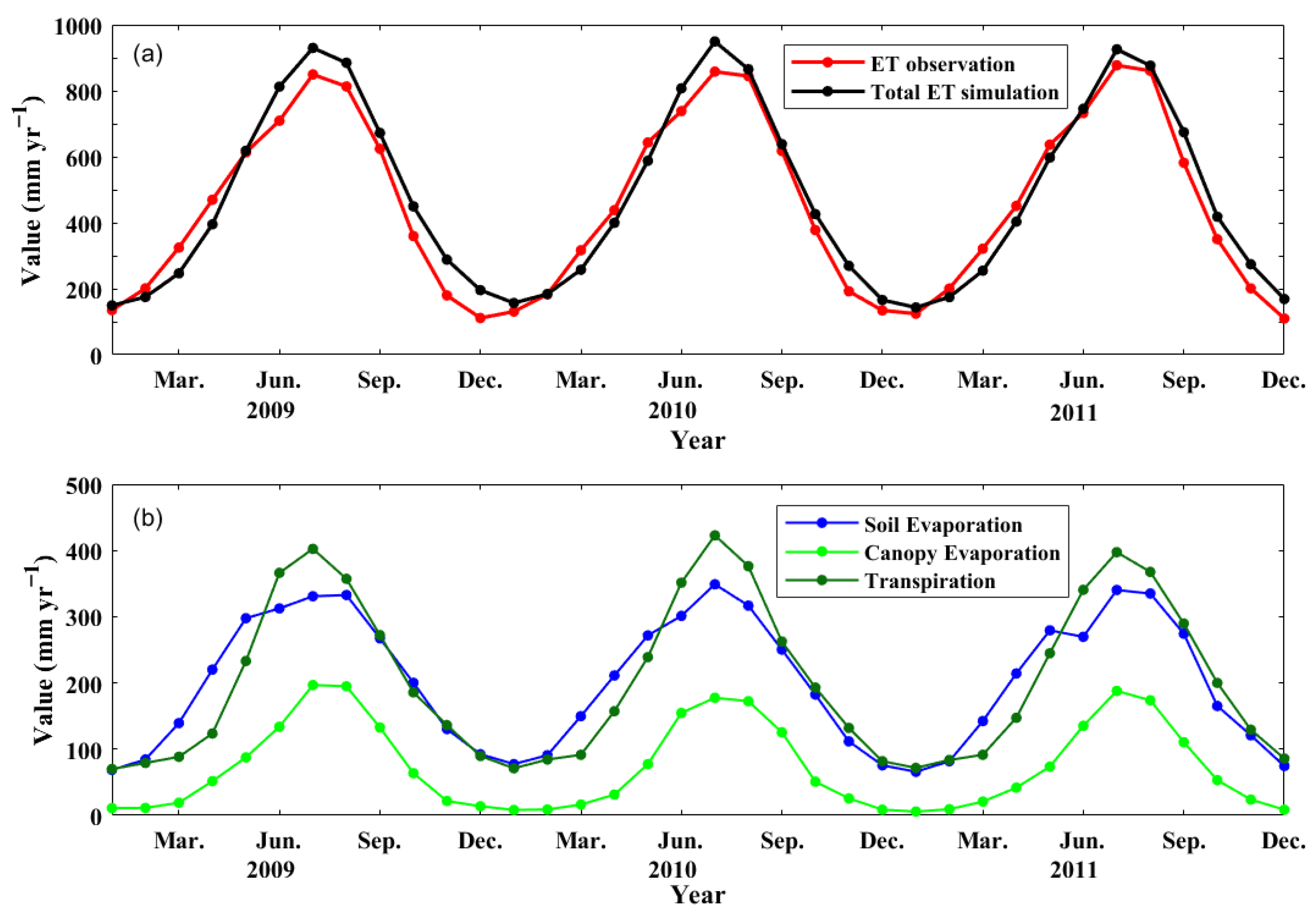
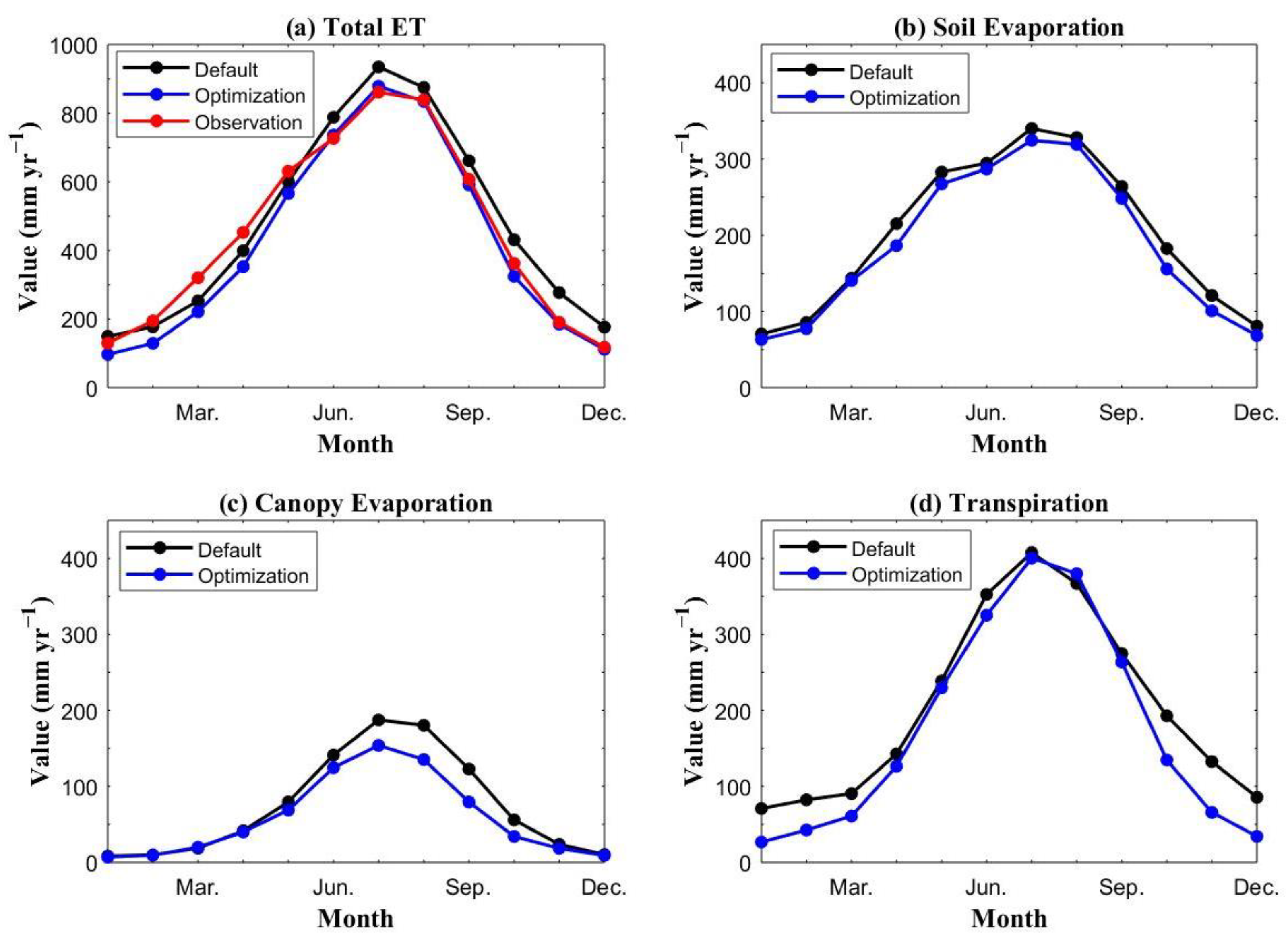
Before conducting sensitivity analysis, the likelihood of CLM4 simulation of ET is first discussed. Figure 2a shows the monthly variation of the total ET observation and simulations from 2009 to 2011 in China. It can be found that the trend of total ET simulations has a consistent seasonal change with observation, although the monthly biases exist between them. The maximum ET occurred in summer (June to August) and the minimum in winter (December to February). Figure 2b shows the monthly variations of three ET component simulations. Besides the same seasonal change, both of the soil evaporation and transpiration was significantly higher than canopy evaporation, and the canopy evaporation was about one-third of the other two components.
Due to no suitable observation used, the results of the three component simulations were compared with those of other literatures. Lawrence et al. [44] found that ET partitioning of 44% transpiration, 39% soil evaporation, and 17% canopy evaporation in global ET simulations is more in line with what one intuitively expect, while the results in Figure 2b were basically consistent with the global partitioning results. China spans 3°–55° N and 73°–136° E, covering the climate characteristics from subfrigid to subtropical zones; therefore, the ET partitioning in China has certain representativeness of global ET partitioning. In addition, according to Lawrence et al. [44], transpiration and soil evaporation are dominant in the agricultural regions and the arid and semiarid regions, respectively. Canopy evaporation is mainly dominant in areas with dense canopies, such as the Amazon and Central America. China is an agricultural country, half of which is arid and semiarid regions. Therefore, it is likely that above 80% ET are from transpiration and soil evaporation in China. There are fewer dense canopy regions in China, and therefore, the lowest canopy evaporation is also thought to be likely. Overall, it is likely that the ET and its three components in China were simulated using the CLM4 model.
Previous studies [29,45] demonstrated that 10× sampled linearly independent parameters were sufficient to obtain reasonable parameter sensitivity results. Therefore, using the GLP uniform sampling method, 380 parameters were sampled from the 38 parameter ranges listed in Table S1. Then, each of the 380 parameter samples was put into the CLM4 to replace the corresponding default parameters for obtaining its ET simulation error. Here, the reference data for the simulation error was the default ET simulation results when the effect of observation error was excluded. As input, the 380 samples and their ET simulation errors were put into the MARS method, and the parameter sensitivity scores were finally obtained.
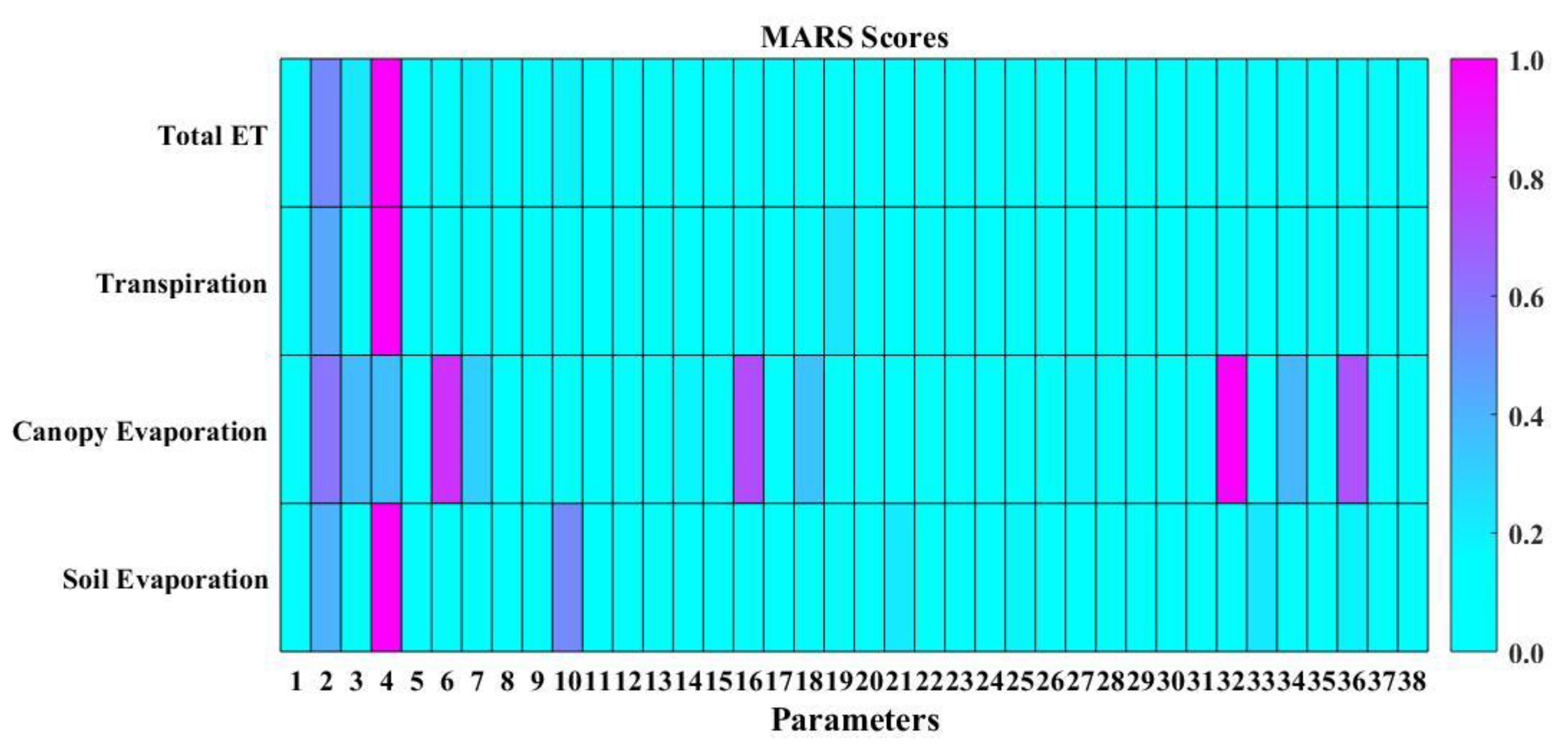
The sensitivity analysis results are shown in Figure 3. The x-axis represents the 38 parameters, and the y-axis are the normalized sensitivity scores of all 38 parameters for total ET and its three component simulations. The most sensitive score was 1, and the least sensitive score was 0. It was seen in Figure 3 that P2 and P4 were common sensitive parameters for total ET and its three component simulations. P10 was sensitive only for the soil evaporation component. For the canopy evaporation simulation, the sensitivity parameters were P2, P6, P16, P32, and P36. Note that there only are two sensitive parameters (i.e., P2 and P4) for total ET. Obviously, the number of sensitive parameters is less. In order to get more parameter supports for further parameter optimization, the sensitive parameters of three ET component simulations were combined. Finally, seven sensitive parameters (P2, P4, P6, P10, P16, P32, and P36) were determined. The names, ranges, and physical meanings of the seven sensitive parameters are listed in Table 1.

3.2. Sensitivity Parameter Optimization Results

After seven sensitive parameters were screened, they were optimized by the ASMO method. One hundred initial samples from the seven sensitive parameter ranges were first sampled by the GLP method, then were respectively put into the CLM4 instead of their default parameter values to obtain the corresponding ET simulation errors. Here, the reference dataset for the simulation errors was the GLEAM ET observations, which differed from that of the parameter sensitivity analysis using the default simulation results as the reference. Next, the response surface model was built by the MARS regression method based on the 100 initial parameter samples and their simulation errors. After that, the search for the optimal parameters of CLM4 was conducted on the continually updated response surface model by adding adaptive sample points obtained by CLM4 simulation.
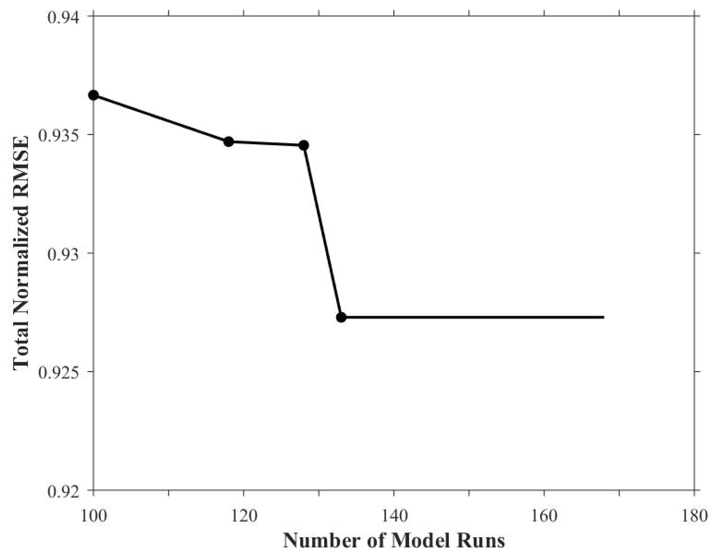
The termination criterion of the search was that the local optimal values remained unchanged after 35 searches (i.e., five times the number of sensitive parameters). Based on this criterion, the optimal parameters of CLM4 for the ET simulation were found; the optimization speed is shown in Figure 4. It was found that the ET simulation was improved by 6.33% over the 100 initial sampled simulations and by a further 7.23% following the additional 33 adaptive search simulations. Overall, the ET simulation was improved by 7.23% using only 133 simulation runs, demonstrating that the ASMO optimization method was very highly effective.

3.3. Comparison Analyses of Optimization Results

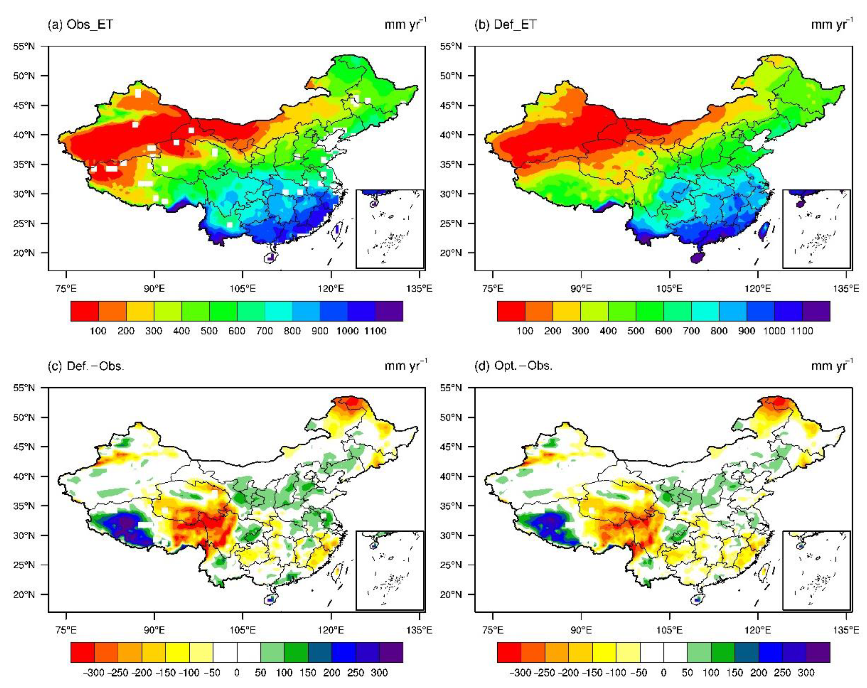
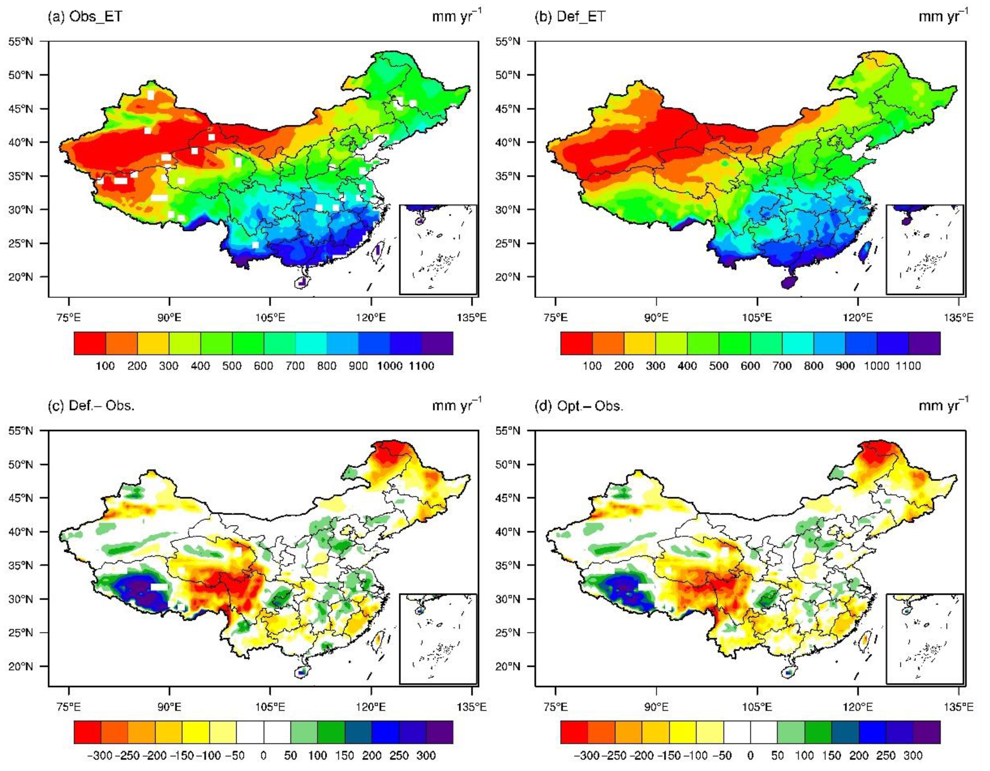
To illustrate the optimization results, comparisons of the spatial distribution of ET simulations from 2009 to 2011 over China were conducted using the CLM4 model with default and optimal parameters. The results are shown in Figure 5. Compared to observations in Figure 5a, the default ET simulations in Figure 5b demonstrated a good spatial consistency: ET values for default simulations gradually increased from northwestern (130.34 mm yr−1) to southeastern (903.62 mm yr−1) China and, for observation, increased from northwestern (135.06 mm yr−1) to southeastern (944.72 mm yr−1) China. It showed that the CLM4 model was suitable for simulating ET in China. However, it was noted that significant differences occurred in the Tibetan Plateau region located in southwestern China.
To obtain a more accurate comparison, two difference experiments were conducted: one was the default simulations minus the observations; the other was the optimal simulations minus the observations. Their results are shown in Figure 5c,d. Overall, the RMSE of the optimal ET simulations for the whole of China was 113.96 mm yr−1, which was lower than 122.89 mm yr−1 for default ET simulations. Figure 5c shows that a significant difference occurs in the Tibetan Plateau, where the RMSE of default simulations is 208.98 mm yr−1. Figure 5d shows that the RMSE of ET simulations in the Tibetan Plateau is decreased to 183.73 mm yr−1 when optimal simulations are used. Using the optimal parameters, the positive bias of ET simulations in the western parts of the Tibetan Plateau decreased from 127.39 to 95.73 mm yr−1. Correspondingly, the negative bias in the eastern parts of the Tibetan Plateau increased from −196.67 to −181.01 mm yr−1. Besides that, the ET simulation errors decreased from 67.18 to 56.83 mm yr−1 in the northern region of China and from 82.64 to 60.63 mm yr−1 in the mid-eastern regions of China. As a whole, these results demonstrated that the optimal parameters obtained by the ASMO method effectively improved the ET simulation of CLM4.
The CLM4 ET simulations were also compared with default and optimal parameters for different months (Figure 6). The red line in Figure 6a represents the observed mean monthly ET values for years 2009 to 2011. The black and blue lines represent the default and optimal mean monthly ET simulation values for years 2009 to 2011, respectively. Comparison of the three lines indicates that the optimal simulation improved the total ET simulation between June and December, and the range of error improvements is from 30.94 in October to 80.63 mm yr−1 in November. Besides that, there were weak negative improvements between January and May, and the range of loss errors was from 13.29 in January to 48.29 mm yr−1 in February. It was also noted that the optimal simulations were smaller than the default simulations for all 12 months of the years 2009–2011, and the range of the difference between them is from 31.43 in March to 106.67 mm yr−1 in October.
Since there was no suitable ET component observation, only the ET component simulations with the optimal and default parameters were compared. The comparison results of the mean monthly simulations for soil evaporation, canopy evaporation, and transpiration are shown in Figure 6b–d. For soil evaporation, the optimal simulations decreased slightly for all 12 months of the year compared with the default simulations. For canopy evaporation and transpiration, a significant decrease using the optimal simulations occurred between July and September and between October and March, respectively. Combining the ET simulation improvements in Figure 6a, it was inferred that the main contributions to ET simulation improvement were from better canopy evaporation simulations between July and September and better transpiration simulations between October and December. It was also noted that the decreases in simulated transpiration using the optimal parameters from January to March had a negative effect on the total ET simulation.
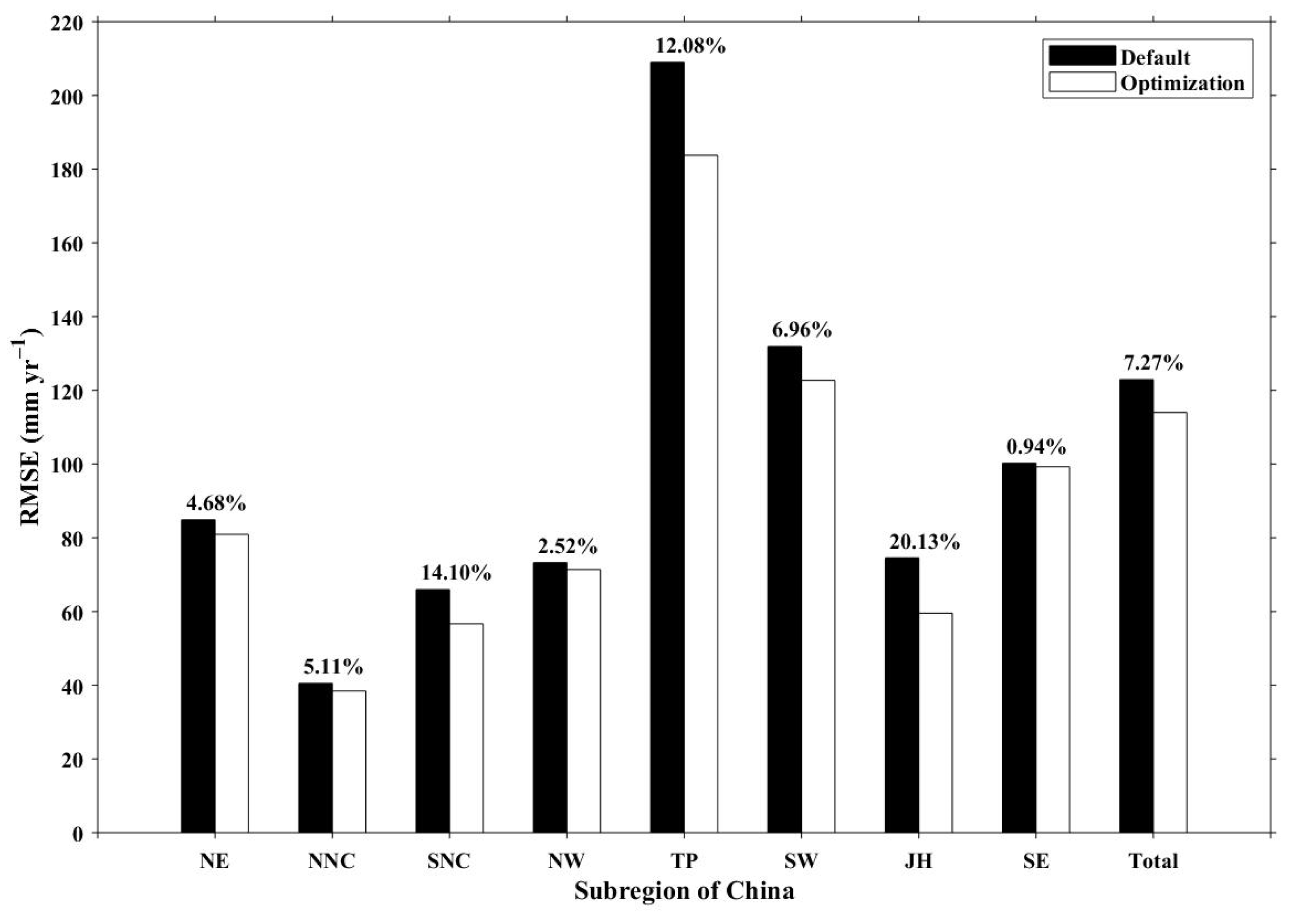
The comparative results for ET simulations of the eight subregions are shown in Figure 7. The overall improvement rate in the simulated ET was 7.27%, and the improvement rates in the eight subregions varied between 0.94% (SE region) and 20.13% (JH region). The most significant improvement rate occurred in the JH region with 20.13%, followed by the SNC region with 14.10% and the TP region with 12.08%. It was noted that the area of the TP region is far greater than that of the SNC region and JH region in Figure 1; therefore, the improvement in the TP region seems to be more attractive. The smallest improvement rates occurred in the SE region (0.94%) and NW region (2.52%). These are explicable that the parameter optimization worked for the simulated ET in regions where the vegetation is affected by significant seasonal changes, as in regions III (SNC) and VII (JH) with deciduous broadleaf forests and for the eastern and western parts of region V (TP) covering the temperate steppe and shrub meadow, respectively. It had little effect where the vegetation has insignificant seasonal changes, as in regions IV (NW) with less vegetation and desert in some places and VIII (SE) with evergreen broadleaf forest. Overall, the improvement in the ET simulations in all of eight subregions demonstrated that the optimal parameters obtained by ASMO method were effective.
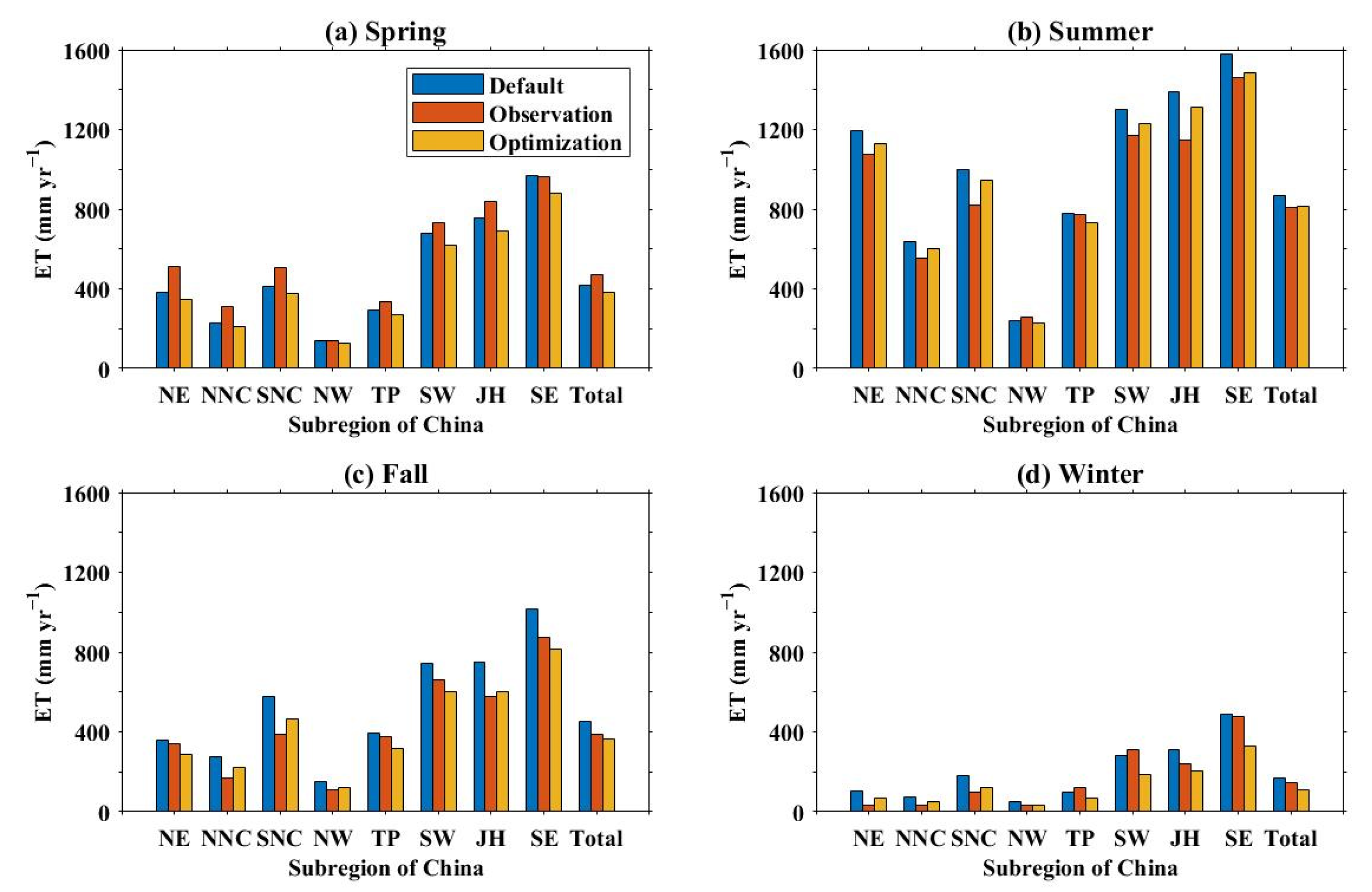
The comparisons of ET simulations with the default and optimal parameters were conducted at a seasonal scale. The results of the ET simulations and observations in the four seasons for China and its eight subregions are shown in Figure 8. Overall, it can be found by comparing the eight subregions that the maximum and minimum ET occurred in the SE and NW regions, respectively. At a seasonal scale, the maximum ET (809.2 mm yr−1) occurred in summer, followed by spring (468.27 mm yr−1) and fall (387.1 mm yr−1) and the minimum ET (147.81 mm yr−1) in winter. With the optimal parameters, the ET simulations in summer and fall were significantly improved and not improved in spring and winter. The ET improvement amount in summer was 49.67 mm yr−1, accounting for 6.14% of the summer observation, and in fall was 48.6 mm yr−1, accounting for 12.56% of the fall observation.
In spring, the default ET simulation values were lower than observations for all of the subregions expect for SE; however, the optimal parameters further reduced the ET simulation values, leading to the increases of ET simulation errors. In the summer, except for the NW and TP subregions with high altitudes, the default ET simulation values of the other six subregions were significantly higher than observations, while the optimal parameters decreased their default ET simulation values, making the ET simulations of these regions improved. The range of improved ET amounts was 36.42 mm yr−1 in NNC to 90 mm yr−1 in JH. Noted that ET simulation values after parameter optimization were still higher than observations.
In the fall, the significant improvements of ET simulations occurred in the SNC subregion, where the ET improvement amount was 113.39 mm yr−1, accounting for 29.4% of SNC observations, and the JH subregion where the ET improvement amount was 147.51 mm yr−1, accounting for 25.44% of JH observations. The vegetation in the two subregions is mainly deciduous broadleaf forest. For the TP subregion, the ET improvement was insignificant, which may be caused by the offset of the positive and negative deviation between the East and West of the TP. In winter, the improvements of the ET simulations mainly occurred in the subregions of the north of China with the smaller ET values. Therefore, the improvement effect was very weak. For the subregions of the south of China, SE and SW had obvious negative improvements, except for JH, with a 14.36% improvement in the absolute value error. Thus, the overall ET simulation was not improved. In addition, it was noted that these improvement rates were not comparable, because their referred observation values were different.

3.4. Validation Analyses of Community Land Model Version 4.0 Optimal Parameters

It was demonstrated above that the optimized parameters were superior to the default parameters for ET simulations in China during the study period 2009–2011. However, it was necessary to test whether the optimized parameters were also appropriate for a different validation period: the two-year period 2014 and 2015 was chosen. Except for simulation time, all other arrangements for this validation experiment were identical to the first (simulation area, CLM4 spatiotemporal resolution and forcing, and validation data).
These comparisons of ET simulations for the period 2014–2015 using the CLM4 model with the default and optimal parameters were conducted based on appropriate GLEAM observational data; the results are shown in Figure 9. With the exception of subregion V (TP), these default ET simulations also showed good spatial consistency with observation, again demonstrating that the CLM4 optimal parameters were suitable for simulating ET in China. To illustrate the difference between the default and optimal ET simulations more accurately, two comparison experiments were conducted: (1) default simulations minus observational data, and (2) optimal simulations minus observational data. The results are shown in Figure 9c,d.
Overall, for the whole of China, the bias of the optimal simulation was lower than that of default simulation. It was also found that the most significant improvement occurred in the TP region with the largest simulation error. Compared with default ET simulations, the optimal simulations reduced the negative bias in the western part of the TP subregion and the positive bias in the eastern part of the TP subregion. In addition, very significantly improved ET simulations were obtained for the SNC and JH subregions. These results are consistent with the conclusions from the comparisons in the optimization period. Therefore, it was concluded that the optimal parameters obtained by the ASMO method were effective and robust.
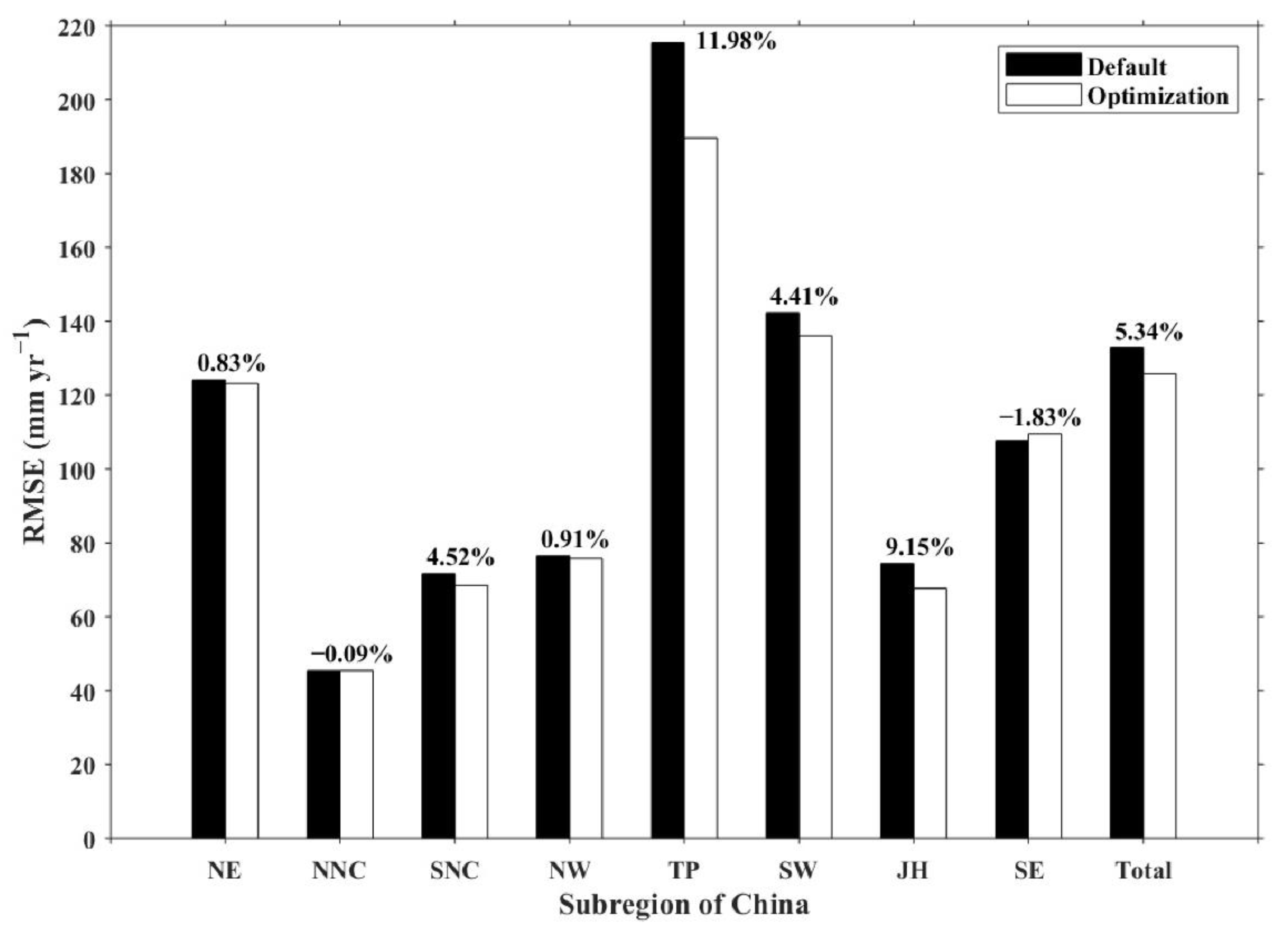
Additionally, comparisons of ET simulations with default and optimal parameters were also conducted for the eight subregions shown in Figure 1. The comparative results are shown in Figure 10. The overall improvement rate of ET simulation was 5.34% for the validation period. The improvement rates varied from −1.83% in the SE subregion to 11.98% in the TP subregion, which was the most significant improvement. The other significant improvements occurred in the JH subregion (9.15%), SNC subregion (4.52%), and SW subregion (4.41%), which were consistent with the improvements found for the optimization period. For the other regions, improvement rates were less than 1%. It was also noted that two of the rates were negative, with the values of −0.09% in the NNC subregion and −1.83% in the SE subregion. The slightly reduced changes to < 2% were outweighed by the improvements over the whole of China; the results for the other six subregions demonstrated that the optimal parameters obtained by the ASMO method were effective and acceptable for the validation period.

3.5. Comparisons between Default and Optimal Parameters

To better demonstrate the parameter variations caused by the optimization procedure, the default and optimal parameters were normalized for the ranges listed in Table 1. Comparisons between the normalized values of the default and optimal parameters of CLM4 model for the ET simulations in China are shown in Figure 11. It was found that the seven parameter variations were inconsistent. The optimal values of the parameters Sy (fraction of water volume that is drained by gravity in an unconfined aquifer) and poro_b (the intercept of mineral soil porosity pedotransfer functions) were higher than the default values. The opposite variations occurred in the parameters fdrai (decay factor of subsurface flow), suc_b (the intercept of pedotransfer functions of saturated mineral soil matric potential), z0mr (ratio of momentum roughness length to canopy top height), rholnir (leaf reflectance: near-infrared radiation), and taulnir (leaf transmittance: near-infrared radiation).

4. Discussion

The effectiveness and robustness of the optimal parameters in improving ET simulations for China are demonstrated above. The physical meaning of the effect of the optimal parameters on the ET simulation of CLM4 are discussed below. As Figure 6 shows, optimization of the parameters predicted an overall reduction in the total ET and its three components. The corresponding physical interpretations are given as follows.
The fdrai (i.e., P2) and Sy (i.e., P4) are two of the sensitive parameters in the simulations of soil evaporation and transpiration shown in Figure 3. Hou et al. [28] reported that when fdrai < 2, it is directly proportional to the amount of simulated ET. Therefore, the lower fdrai value in Figure 11 would be expected to decrease the default simulated ET amount. In a physical sense, fdrai is related to drainage in the CLM4 model, such that lower fdrai values correspond to increased drainage. As a result, more water in shallow aquifers recharges the groundwater downward, leading to a decrease of soil water and, consequently, lower soil evaporation and transpiration.
Sy (specific yield) represents the volumetric proportion of water in the soil that is free to move by gravity. When Sy increases, more free water is generated in shallow aquifers. Under the action of gravity, the increased volume of free water recharges the underlying aquifer and, thus, has the same effect as the fdrai value discussed above.
The parameters poro_b (i.e., P6), z0mr (i.e., P16), rholnir (i.e., P32), and taulnir (i.e., P36) mainly work in the simulation of canopy evaporation, as shown in Figure 3. The poro_b parameter refers to soil porosity. The larger soil porosity signified by a greater poro_b value has the effect of increasing surface water vapor flux, as well as relative humidity at canopy height. The difference between saturated water vapor pressure and relative humidity thus decreases at canopy height, resulting in lower canopy evaporation. The z0mr value represents the ratio of momentum roughness length to canopy-top height, which is reduced when z0mr decreases. Correspondingly, the aerodynamic resistance is reduced, resulting in lowered leaf-moisture transfer and, thus, weaker canopy evaporation. The rholnir and taulnir parameters represent the energy of leaf reflectance (rholnir) and transmittance (taulnir) to near-infrared radiation. When both of them decrease, the upward and downward diffuse fluxes on leaves caused by near-infrared radiation are reduced. As a result, heat transfer between the leaves and the atmosphere is also reduced, leading to less canopy evaporation.
The parameter suc_b (i.e., P10) is sensitive to the soil evaporation simulation, as shown in Figure 3, and represents the intercept of the pedotransfer functions of saturated mineral soil matric potential; it is therefore related to the soil matric potential. In CLM4, the saturated mineral soil matric potential is inversely proportional to suc_b, so that a smaller suc_b represents an increase in soil matric potential and, correspondingly, increases the adsorption force of soil particles to water, and thus, less water escapes to the atmosphere.
Although the overall improvement ratio (7.27% for optimization and 5.34% for validation) seems to be relatively small, the optimal parameters obtained by ASMO were thought to be useful. Two reasons are given: (1) the point of improvement rate. The overall improvements of 7.27% and 5.34% are the national average values. It can be found from Figure 7 and Figure 10 that the improvement rates of some subregions (e.g., TP, SNC, and JH) are more than 10% or even 20%, which is not ignored. Additionally, the ET simulations errors of the three regions in the spatial distribution are also most significant (see Figure 5 and Figure 9). For the rest five subregions, the improvement rates are less than 5%, which is thought to be no improvement. Therefore, the overall improvement in China is low when all of the errors in eight subregions are averaged. In addition, it is also acceptable that the optimal parameters significantly improve the ET simulations in the subregions with the larger ET simulation errors, while having no obvious damage for the ET simulations of the other subregions, (2) The point of physical sense; the previous results have shown that, on the one hand, the optimal parameters work in the regions whose vegetation have obvious seasonal changes, such as the SNC and JH with the temperate, deciduous broadleaf forest vegetation and the eastern and western parts of TP covering the temperate steppe and shrub meadow, respectively; on the other hand, the optimal parameters does not work in the regions whose vegetation have no obvious seasonal changes, such as such as the northern part of NE (subfrigid coniferous forest) and SE (subtropical evergreen broadleaf forest). Therefore, the final results are low improvements in China. The optimal parameters are ineffective to ET simulations for the vegetation without seasonal changes. The reason may be that some parameters related to the vegetation without seasonal changes are missed in this study or the relevant parameterization schemes need to be further improved.
The presented approach in this study is more inclined to adjust the parameters of the land-scale ET model at the month or even annual scale. The reasons are given as follows. The ET estimation formula (e.g., Penman-Monteith formula) at the field scale uses the observational variables at instantaneous (hourly) or even daily temporal scales as inputs. Therefore, the ET calculation speed at the field scale is very fast. Tens of thousands of runs are usually completed in servers in hours or days. Thus, the traditional parameter optimization method (e.g., SCE-UA) requiring ten-thousand model runs is enough to adjust the parameters of the field-scale ET formula. However, the ET simulation of the land surface model at the land and monthly scales is very time-consuming. Since the land surface model requires evaluating all land physical equations at each time step to ensure a water and energy budget balance, the solved variables as inputs are then put into the ET formula. In addition, the land surface models are usually used to conduct long-term simulations at a monthly or even annual scale for presenting the climatic characteristics of the output variables. Therefore, the ET simulations of the land surface model at the monthly scale are very expensive. Thus, the traditional parameter optimization method is not suitable for adjusting their parameters. It seems that the only efficient solution at present is to use our proposal approach: combing the parameter screen method and the highly efficient optimization method for screened sensitivity parameters.

5. Conclusions

In this study, a highly efficient parameter optimization framework was applied to improve the ET simulation of the CLM4 model for China. The CLM4 is a model at a land scale, and therefore, the monthly ET observation was used to evaluate the ET simulations. Results showed that seven sensitive parameters from 38 adjustable parameters for simulating ET were first screened using the MARS sensitivity analysis method. Then, these seven parameters were optimized using the highly efficient ASMO method. After optimizing the parameters, three aspects of the default and optimal ET simulations were compared: spatial distribution, mean monthly variation, and subregional difference. Finally, the optimal parameters were validated by comparing the simulated ET for another time period and discussing the physical interpretations of the parameter perturbations.
The CLM4 is a complex land surface model with detailed physical descriptions, and therefore, its simulation is very time-consuming, especially for the simulation of large areas over a long period. It is very difficult to conduct a parameter optimization for CLM4 using traditional optimization methods that require tens of thousands of model runs. In this study, an ASMO parameter optimization method was applied to CLM4 parameters to improve ET simulations in China. The results demonstrated that the optimal parameters for CLM4 required only 133 model runs, made up of 100 initial sampled runs and 33 adaptive optimization runs. Therefore, the ASMO parameter optimization method was found to be highly efficient.
Comparisons between the default and optimal ET simulations were conducted for two time periods: optimization for 2009–2011 and validation for 2014–2015. For the optimization period, the default ET simulations were improved by 7.27% using the optimal parameters. Based on the differences of spatial ET simulations, it was found that the optimal simulations overall reduced the bias of the default ET simulations. The largest bias occurred in the TP subregion. By comparing the mean monthly ET simulation results, it was found that improved ET simulations occurred between June and December, mainly attributable to better simulations of canopy evaporation for July to September, and transpiration simulations for October to December. Comparisons of ET simulations in the eight subregions found that the most significant improvements occurred in the TP, JH, and SNC subregions, where the vegetation has significant seasonal change. The least significant improvements were in the SE subregion with an evergreen broadleaf forest and the NW subregion with less vegetation and some desert. Comparisons of ET simulations at a seasonal scale found that the ET simulations in the summer and fall were significantly improved and not improved in the spring and winter. For the validation period, the simulated ET was improved by 5.34%. Comparisons of ET simulations for the whole of China and for its eight subregions were consistent with those in the optimization period. Therefore, it is concluded that the optimal parameters obtained by the ASMO method were effective and robust.
This study has demonstrated that the ASMO method is an efficient way of conducting parameter optimization for the complex CLM4 model. The optimal parameters effectively improved ET simulation for the CLM4 model over China. However, some limitations should be noted: For example, although the optimized ET simulations showed improvements over the whole of China and even its eight subregions, there were exceptions. ET simulation was not improved for all months; also, the verification data consisted only of total ET observations without three-component observations due to the lack of an accurate data resource. It may appear the case that the total ET simulation is improved, while one of the component simulations shows significant worsening. Therefore, future work will focus on multiobjective variable optimization.

Supplementary Materials

The following are available online at https://www.mdpi.com/2073-4441/12/4/943/s1: Table S1: Tunable parameters and their variability ranges for CLM4.

Author Contributions

Data curation, C.Z. and Z.D.; methodology, Z.D. and W.G.; formal analysis, Z.D. and Z.X.; writing—original draft preparation, C.Z. and Z.D.; and supervision, Z.D. and Q.D. All authors have read and agreed to the published version of the manuscript.

Funding

This research was supported by the National Natural Science Foundation of China (grant no. 41930970), the National Key R&D Program of China (grant no. 2019YFA0606900), and the Second Tibetan Plateau Scientific Expedition and Research Program (grant no. 2019QZKK0405)

Acknowledgments

GLEAM evapotranspiration data are available online at https://www.gleam.eu; CRU-NCEP data are available online at https://rda.ucar.edu/datasets/ds314.3.

Conflicts of Interest

The authors declare no conflicts of interest.

References

  1. Oki, T.; Kanae, S. Global hydrological cycles and world water resources. Science 2006, 313, 1068–1072. [Google Scholar] [CrossRef] [PubMed] [Green Version]
  2. Jasechko, S.; Sharp, Z.D.; Gibson, J.J.; Birks, S.J.; Yi, Y.; Fawcett, P.J. Terrestrial water fluxes dominated by transpiration. Nature 2013, 496, 347–350. [Google Scholar] [CrossRef] [PubMed]
  3. Trenberth, K.E.; Fasullo, J.T.; Kiehl, J. Earth’s global energy budget. B. Am. Meteorol. Soc. 2009, 90, 311–324. [Google Scholar] [CrossRef]
  4. Monteith, J.L. Evaporation and Environment. In The State and Movement of Water in Living Organism; Fogg, B.D., Ed.; Symposium of the Society of Experimental Biology XIX: Cambridge, UK, 1965; pp. 205–234. [Google Scholar]
  5. Priestley, C.; Taylor, R.J. On the assessment of surface heat flux and evaporation using large-scale parameters. Mon. Weather Rev. 1972, 100, 81–92. [Google Scholar] [CrossRef]
  6. Wang, K.; Dickinson, R.E. A review of global terrestrial evapotranspiration: Observation, modeling, climatology, and climatic variability. Rev. Geophys. 2012, 50, 1131–1151. [Google Scholar] [CrossRef]
  7. Niu, G.Y.; Yang, Z.L.; Dickinson, R.E.; Gulden, L.E.; Su, H. Development of a simple groundwater model for use in climate models and evaluation with Gravity Recovery and Climate Experiment data. J. Geophys. Res. Atmos. 2007, 112, D07103. [Google Scholar] [CrossRef]
  8. Christensen, N.S.; Wood, A.W.; Voisin, N.; Lettenmaier, D.P. The effects of climate change on the hydrology and water resources of the Colorado River basin. Climatic Change 2004, 62, 337–363. [Google Scholar] [CrossRef]
  9. Budyko, M.I. The Heat Balance of the Earth’s Surface; U.S. Dept. of Commerce: Washington, DC, USA, 1958.
  10. Sellers, P.J.; Randall, D.A.; Collatz, G.J.; Berry, J.A.; Field, C.B.; Dazlich, D.A.; Zhang, C.; Collelo, G.D.; Bounoua, L. A revised land surface parameterization (SiB2) for atmospheric GCMs. Part I: Model formulation. J. Climate 1996, 9, 676–705. [Google Scholar] [CrossRef]
  11. Niyogi, D.; Alapaty, K.; Raman, S.; Chen, F. Development and evaluation of a coupled photosynthesis-based gas exchange evapotranspiration model (GEM) for mesoscale weather forecasting applications. J. Appl. Meteorol. Clim. 2009, 48, 349–368. [Google Scholar] [CrossRef] [Green Version]
  12. Oleson, K.W.; Lawrence, D.M.; Bonan, G.B.; Flanner, M.G.; Kluzek, E.; Lawrence, P.J.; Levis, S.; Swenson, S.C.; Thornton, P.E.; Dai, A.; et al. Technical Description of Version 4.0 of the Community Land Model (CLM); Rep. NCAR/TN-478 + STR; NCAR: Boulder, CO, USA, 2010; p. 257. [Google Scholar]
  13. Dirmeyer, P.A.; Dolman, A.J.; Sato, N. The pilot phase of the global soil wetness project. B. Am. Meteorol. Soc. 1999, 80, 851–878. [Google Scholar] [CrossRef] [Green Version]
  14. Amthor, J.S.; Chen, J.M.; Clein, J.S.; Frolking, S.E.; Goulden, M.L.; Grant, R.F.; Kimball, J.S.; King, A.W.; McGuire, A.D.; Nikolov, N.T.; et al. Boreal forest CO2 exchange and evapotranspiration predicted by nine ecosystem process models: Intermodel comparisons and relationships to field measurements. J. Geophys. Res. Atmos. 2001, 106, 33623–33648. [Google Scholar] [CrossRef] [Green Version]
  15. Charney, J.G. Dynamical forecasting by numerical process. In Compendium of Meteorology; Malone, T.F., Ed.; American Meteorological Society: Boston, MA, USA, 1951; pp. 470–482. [Google Scholar]
  16. Rodell, M.; Houser, P.R.; Jambor, U.; Gottschalck, J.; Mitchell, K.; Meng, C.; Arsenault, K.; Cosgrove, B.; Radakovich, J.; Bosilovich, M.; et al. The global land data assimilation system. Bull. Am. Meteorol. Soc. 2004, 85, 381–394. [Google Scholar] [CrossRef] [Green Version]
  17. Xu, T.; Liu, S.; Liang, S.; Qin, J. Improving predictions of water and heat fluxes by assimilating MODIS land surface temperature products into the common land model. J. Hydrometeorol. 2011, 12, 227–244. [Google Scholar] [CrossRef]
  18. Stensrud, D.J. Parameterization Schemes: Keys to Understanding Numerical Weather Prediction Models; Cambridge University Press: Cambridge, UK, 2007. [Google Scholar]
  19. Zeng, Y.; Xie, Z.; Yu, Y.; Liu, S.; Wang, L.; Zou, J.; Qin, P.; Jia, B. Effects of anthropogenic water regulation and groundwater lateral flow on land processes. J. Adv. Model. Earth Syst. 2016, 8, 1106–1131. [Google Scholar] [CrossRef]
  20. Liu, J.; Jia, B.; Xie, Z.; Shi, C. Ensemble simulation of land evapotranspiration in China based on a multi-forcing and multi-model approach. Adv. Atmos. Sci. 2016, 33, 673–684. [Google Scholar] [CrossRef]
  21. Raftery, A.E.; Gneiting, T.; Balabdaoui, F.; Polakowski, M. Using Bayesian model averaging to calibrate forecast ensembles. Mon. Weather Rev. 2005, 133, 1155–1174. [Google Scholar] [CrossRef] [Green Version]
  22. Högström, U.; Bergström, H. Organized turbulence structures in the near-neutral atmospheric surface layer. J. Atmos. Sci. 1996, 53, 2452–2464. [Google Scholar] [CrossRef] [Green Version]
  23. Duan, Q.; Sorooshian, S.; Gupta, V.K. Optimal use of the SCE-UA global optimization method for calibrating watershed models. J. Hydrol. 1994, 158, 265–284. [Google Scholar] [CrossRef]
  24. Lettenmaier, D.; Lohmann, D.; Wood, E.F.; Liang, X. PILPS-2c Workshop Report; Princeton University: Princeton, NJ, USA, 1996. [Google Scholar]
  25. Gupta, H.V.; Bastidas, L.A.; Sorooshian, S.; Shuttleworth, W.; Yang, Z. Parameter estimation of a land surface scheme using multicriteria methods. J. Geophys. Res. Atmos. 1999, 104, 19491–19503. [Google Scholar] [CrossRef] [Green Version]
  26. Jackson, C.; Xia, Y.; Sen, M.K.; Stoffa, P.L. Optimal parameter and uncertainty estimation of a land surface model: A case study using data from Cabauw, Netherlands. J. Geophys. Res. Atmos. 2003, 108, 4583. [Google Scholar] [CrossRef] [Green Version]
  27. Liu, Y.; Gupta, H.V.; Sorooshian, S.; Bastidas, L.A.; Shuttleworth, W.J. Constraining land surface and atmospheric parameters of a locally coupled model using observational data. J. Hydrometeorol. 2005, 6, 156–172. [Google Scholar] [CrossRef]
  28. Hou, Z.; Huang, M.; Leung, L.R.; Lin, G.; Ricciuto, D.M. Sensitivity of surface flux simulations to hydrologic parameters based on an uncertainty quantification framework applied to the Community Land Model. J. Geophys. Res. Atmos. 2012, 117, 156–169. [Google Scholar] [CrossRef]
  29. Li, J.; Duan, Q.; Gong, W.; Ye, A.; Dai, Y.; Miao, C.; Di, Z.; Tong, C.; Sun, Y. Assessing parameter importance of the Common Land Model based on qualitative and quantitative sensitivity analysis. Hydrol. Earth Syst. Sc. 2013, 17, 3279–3293. [Google Scholar] [CrossRef] [Green Version]
  30. Gan, Y.; Liang, X.; Duan, Q.; Choi, H.I.; Dai, Y.; Wu, H. Stepwise sensitivity analysis from qualitative to quantitative: Application to the terrestrial hydrological modeling of a Conjunctive Surface-Subsurface Process (CSSP) land surface model. J. Adv. Model. Earth Syst. 2015, 7, 648–669. [Google Scholar] [CrossRef] [Green Version]
  31. Wang, C.; Duan, Q.; Gong, W.; Ye, A.; Di, Z.; Miao, C. An evaluation of adaptive surrogate modeling based optimization with two benchmark problems. Environ Modell. Softw. 2014, 60, 167–179. [Google Scholar] [CrossRef] [Green Version]
  32. Gong, W.; Duan, Q.; Li, J.; Wang, C.; Di, Z.; Dai, Y.; Ye, A.; Miao, C. Multi-objective parameter optimization of Common Land Model using adaptive surrogate modeling. Hydrol. Earth Syst. Sc. 2015, 19, 2409–2425. [Google Scholar] [CrossRef] [Green Version]
  33. Martens, B.; Miralles, D.G.; Lievens, H.; van der Schalie, R.; de Jeu, R.A.M.; Fernández-Prieto, D.; Beck, H.E.; Dorigo, W.; Verhoest, N. GLEAM v3: Satellite-based land evaporation and root-zone soil moisture. Geosci. Model Dev. 2017, 10, 1903–1925. [Google Scholar] [CrossRef] [Green Version]
  34. Viovy, N. CRUNCEP Version 7-Atmospheric Forcing Data for the Community Land Model; Research Data Archive at the National Center for Atmospheric Research, Computational and Information Systems Laboratory: Boulder, CO, USA, 2018. [Google Scholar] [CrossRef]
  35. Friedman, J.H. Multivariate adaptive regression splines. Ann. Statist. 1991, 19, 1–67. [Google Scholar] [CrossRef]
  36. Fang, K.; Lin, D.K.J.; Winker, P.; Zhang, Y. Uniform design: Theory and application. Technometrics 2000, 42, 237–248. [Google Scholar] [CrossRef]
  37. Di, Z.; Duan, Q.; Gong, W.; Ye, A.; Miao, C. Parametric sensitivity analysis of precipitation and temperature based on multi-uncertainty quantification methods in the weather research and forecasting model. Sci. China Earth Sci. 2017, 60, 876–898. [Google Scholar] [CrossRef]
  38. Di, Z.; Duan, Q.; Wang, C.; Ye, A.; Miao, C.; Gong, W. Assessing the applicability of WRF optimal parameters under the different precipitation simulations in the Greater Beijing Area. Clim. Dyn. 2018, 50, 1927–1948. [Google Scholar] [CrossRef]
  39. Di, Z.; Duan, Q.; Shen, C.; Xie, Z. Improving WRF typhoon precipitation and intensity simulation using a surrogate-based automatic parameter optimization method. Atmosphere 2020, 11, 89. [Google Scholar] [CrossRef] [Green Version]
  40. Ma, Z.; Huang, G.; Gan, W.; Chen, M. Multi-scale temporal characteristics of the dryness/wetness over Northern China during the last century. Chin. J. Atmos. Sci. 2005, 29, 671–681. (In Chinese) [Google Scholar]
  41. Peters-Lidard, C.D.; Zion, M.S.; Wood, E.F. A soil-vegetation-atmosphere transfer scheme for modeling spatially variable water and energy balance processes. J. Geophys. Res. Atmos. 1997, 102, 4303–4324. [Google Scholar] [CrossRef]
  42. Chen, F.; Dudhia, J. Coupling an advanced land surface-hydrology model with the Penn State–NCAR MM5 modeling system part I: Model implementation and sensitivity. Mon. Wea. Rev. 2001, 129, 569–585. [Google Scholar] [CrossRef] [Green Version]
  43. Huang, M.; Hou, Z.; Leung, L.R.; Ke, Y.; Liu, Y.; Fang, Z.; Sun, Y. Uncertainty analysis of runoff simulations and parameter identifiability in the Community Land Model: Evidence from MOPEX basins. J. Hydrometeorol. 2013, 14, 1754–1772. [Google Scholar] [CrossRef]
  44. Lawrence, D.M.; Thornton, P.E.; Oleson, K.W.; Bonan, G.B. The partitioning of evapotranspiration into transpiration, soil evaporation, and canopy evaporation in a GCM: Impacts on land–atmosphere interaction. J. Hydrometeorol. 2007, 8, 862–880. [Google Scholar] [CrossRef]
  45. Gan, Y.; Duan, Q.; Gong, W.; Tong, C.; Sun, Y.; Chu, W.; Ye, A.; Miao, C.; Di, Z. A comprehensive evaluation of various sensitivity analysis methods: A case study with a hydrological model. Environ. Modell. Softw. 2014, 51. [Google Scholar] [CrossRef] [Green Version]
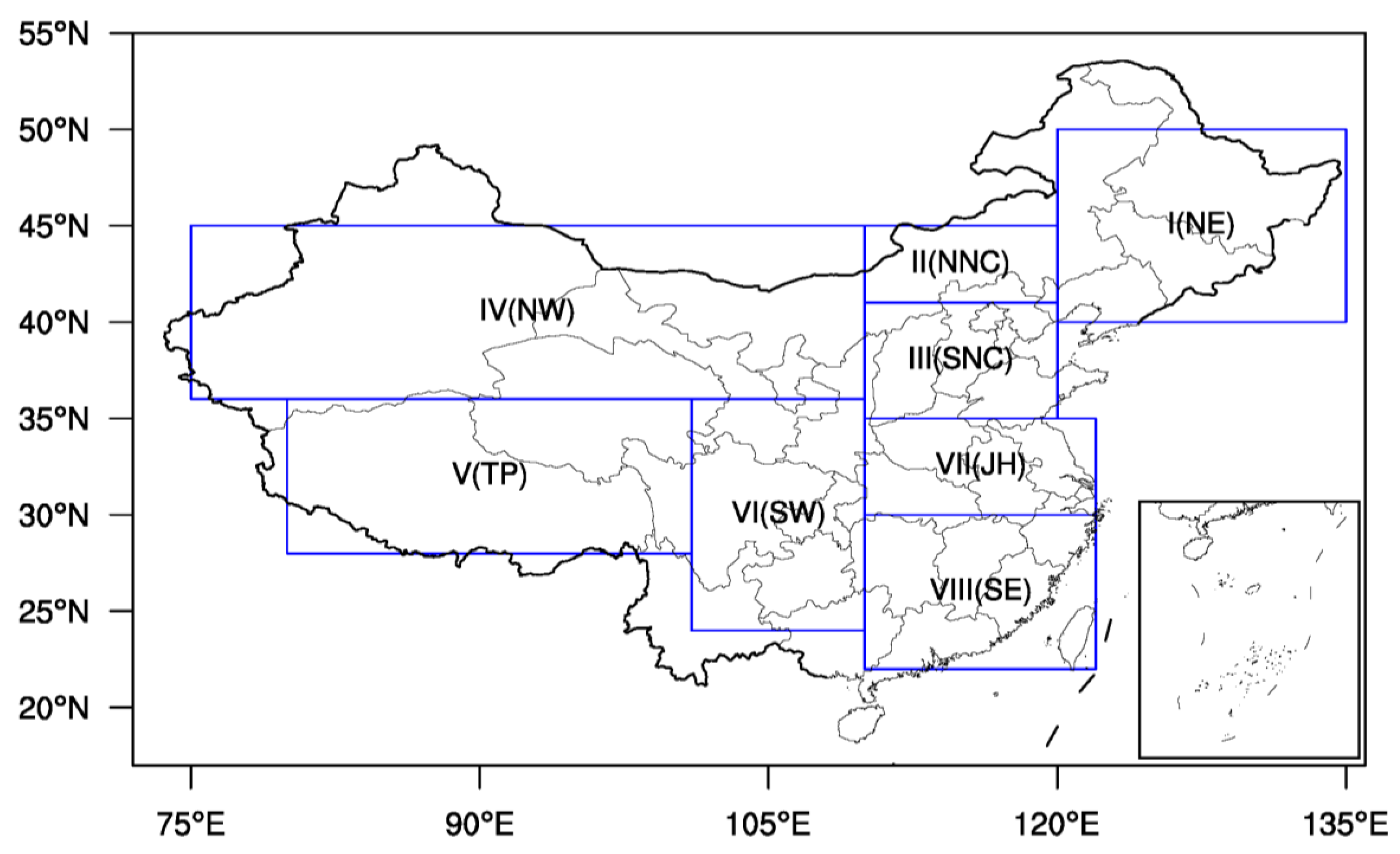
Figure 1. The study domain and its eight subregions marked with blue boxes. The eight subregions are (I) northeastern (NE, 40°–50° N, 120°–135° E), (II) northern part of North China (NNC, 41°–45° N, 110°–120° E), (III) southern part of North China (SNC, 35°–41° N, 110°–120° E), (IV) northwestern (NW, 36°–45° N, 75°–110° E), (V) Tibetan Plateau (TP, 28°–36° N, 80°–101° E), (VI) southwestern (SW, 24°–36° N, 101°–110° E), (VII) Jianghuai region (JH, 30°–35° N, 110°–122° E), and (VIII) southeastern (SE, 22°–30° N, 110°–120° E).
Water 12 00943 g001
Figure 2. Monthly variation of the evapotranspiration (ET) observation and simulations from 2009 to 2011 in China: (a) total evapotranspiration observation and simulation; and (b) simulations of evapotranspiration’s three components, including soil evaporation, canopy evaporation, and transpiration.
Water 12 00943 g002
Figure 3. Normalized sensitivity scores of 38 parameters for total evapotranspiration and its three component simulations. MARS = multivariate adaptive regression spline method.
Water 12 00943 g003
Figure 4. Optimization speed for evapotranspiration simulation in Community Land Model version 4.0 using the adaptive surrogate modeling-based optimization method.
Water 12 00943 g004
Figure 5. Comparisons of the spatial distribution of evapotranspiration simulations from 2009 to 2011 over China using Community Land Model version 4.0 model with default and optimal parameters: (a) observations. The white grids in China represent the missing values, (b) default simulations, (c) bias of default simulations minus observations, and (d) bias of optimal simulations minus observations.
Water 12 00943 g005
Figure 6. Comparisons between mean monthly evapotranspiration simulated values for 2009–2011 using Community Land Model version 4.0 model with default and optimal parameters for: (a) total evapotranspiration, (b) soil evaporation, (c) canopy evaporation, and (d) transpiration.
Water 12 00943 g006
Figure 7. Comparisons of evapotranspiration simulations using default parameters and optimal parameters in the eight subregions of China.
Water 12 00943 g007
Figure 8. Comparisons of the evapotranspiration at the seasonal scale among default simulations, optimal simulations, and observations for China and its eight subregions for: (a) Spring, (b) Summer, (c) Fall, and (d) Winter.
Water 12 00943 g008
Figure 9. Comparisons of the spatial distribution of evapotranspiration simulations from 2014 to 2015 over China using Community Land Model version 4.0 model with default and optimal parameters: (a) observations. The white grids in China represent the missing values, (b) default simulations, (c) bias of default simulations minus observations, and (d) bias of optimal simulations minus observations.
Water 12 00943 g009
Figure 10. Comparisons of evapotranspiration simulations using default parameters and optimal parameters in the eight subregions of China. 2014–2015.
Water 12 00943 g010
Figure 11. Comparisons of normalized optimal and default parameter values of Community Land Model version 4.0 model for the evapotranspiration simulations in China.
Water 12 00943 g011
Table 1. List of sensitive parameters for the evapotranspiration simulation in the Community Land Model version 4.0.
IndexParameterDefaultRangeDescription
P2fdrai2.5(0.1, 5)Decay factor of subsurface flow (m−1)
P4Sy0.2(0.02, 0.27)Fraction of water volume drained by gravity in an unconfined aquifer
P6poro_b0.489(0.4401, 0.5379)The intercept of mineral soil porosity pedotransfer function
P10suc_b1.88(1.692, 2.068)The intercept of pedotransfer function of saturated mineral soil matric potential
P16z0mr1(0.7, 1.3)Ratio of momentum roughness length to canopy top height
P32rholnir1(0.7, 1.3)Leaf reflectance: near-infrared radiation
P36taulnir1(0.7, 1.3)Leaf transmittance: near-infrared radiation