1. Introduction
In a global database of landslide disasters given by Froude and Petley (2018) [
1], three–quarters of all landslide events between 2004 to 2016 occurred in Asian countries, with substantial events in the Himalayas. Indian Himalayas are highly susceptible to landslides which are triggered primarily by rainfall [
2] and Sikkim and Darjeeling Himalayas are among the most highly vulnerable landslide zones. Due to rapid urbanization and increase in population in such areas, landslides and associated loss are an increasing concern [
3] and early warning systems are regarded as a promising tool for landslide forecasting and risk management [
4].
Rainfall being the most common triggering factor for landslides, early warning systems are typically based on empirical rainfall thresholds that describe the interaction between the primary cause (rainfall) and the final effect (landslide). In a few words, a triggering threshold is represented by a mathematical equation describing the critical rainfall condition above which landslides are triggered. The only input data used for the threshold definition are a dataset of rainfall recordings and a catalogue of landslides for which the time and location of occurrence are known with sufficient approximation. This approach completely bypasses the physical mechanism of triggering, thus simplifying the modeling effort, the computational resources required, and the amount of data needed for the analysis [
5].
During the last few decades, many attempts were made across the world to define critical rainfall thresholds based on a number of different rainfall parameter, but the most common are intensity and duration (ID thresholds) [
6,
7,
8,
9,
10,
11,
12,
13], total event rainfall and duration (ED thresholds) [
14,
15,
16,
17,
18] and antecedent rainfall [
19,
20,
21,
22]. The selection of the optimal rainfall parameters which are used for defining the threshold depends mainly on the landslide typology and physical characteristics of the region. It is well accepted that shallow landslides and debris flows are triggered by high intensity-short rainfalls and deep-seated landslides occur as a result of less intense rain over a long time [
16,
23,
24]
When an area is prone to both shallow and rapid and deep-seated and slow moving landslides, a threshold model which can accommodate the effect of both the cases should be defined. A model that holds this characteristic is SIGMA (sistema integrato gestione monitoraggio allerta—integrated system for management, monitoring and alerting), which was developed for managing the risk associated with landslides triggered by rainfall in the Emilia-Romagna Region, Italy [
23,
25,
26]. The model takes cumulative rainfall as input, and it considers the long-term and short-term behavior in order to account for shallow and deep landslides, respectively. Another important advantage of this method is the indication of warning level. The model can be calibrated with respect to the severity of landslides and can be used for developing regional site specific thresholds.
An ongoing research continuously produced new upgrades and optimization of the model SIGMA [
19,
26,
27], making it possible to be used across the world for landslide hazard warning. However, to our knowledge, the model has never been applied outside Italy, thus leaving the claimed flexibility of application only theoretical. Hence, this study applies the SIGMA model to Kalimpong town in the Darjeeling Himalayas and thus tests the exportability of the SIGMA model in different climatic and geomorphological settings.
2. Study Area and Input Data
Kalimpong town is a part of the Kalimpong district of West Bengal state, India, as shown in
Figure 1. This hilly town belongs to Darjeeling Himalayas, hemmed between rivers Tista in the west and Relli in the east, with an elevation ranging from 355 m to 1646 m above mean sea level. The slopes in the western face of the town are steep, while the eastern slopes are gentle.
The geological setting of the region is associated with the evolution of Darjeeling Himalayan ranges. Precambrian high-grade gneiss and quartzite, calc–silicate and quartzite, high-grade schist phyletic etc. are the dominant rock types found in the region [
28]. Upper sedimentary layers of the young folded mountains get eroded during heavy rainfalls. The area consists of several joints and cracks that accelerates the weathering of the rock and the formation of unconsolidated matter [
29]. The bedrock throughout the study area is composed of Daling series quartz mica schist of golden to silver colors [
30]. The inclination of bed towards the east and northeast varies from 20° near river Tista to about 40° towards town. These slopes in can be morphometrically classified into escarpment category A (>45°), steep slope category B (30°–45°), moderate steep slope category C (20°–30°) and gentle slope category D (10°–20°). Silt to medium grained sand and loam constitutes a major portion of the topsoil of the area. According to GSI, more than 60% of the region comprises colluvium followed by older debris (24%) and young debris (2.5%). This geomorphological setting makes the region very prone to landslides, and rainfall is the main triggering factor.
The geology of the area allows rainwater to percolate, increasing the pore pressure, therefore the shear strength of the soil decreases. The change in water content due to intense rainfall leads to the saturation of material and a sudden increase in the unit weight. This mechanism reduces the stability and resistance of parent rocks. The average annual precipitation in this area was observed to be 1872 mm during the study period, and the drainage density of the region is also very high. The area is drained by numerous mountainous natural streams (kholas) and their tributaries (jhoras). The precipitation with daily accuracy was collected for this study from the rain gauge maintained in Tirpai, Kalimpong (Save The Hills). The months from June to September are considered a monsoon period and the monthly rainfall from 2010 to 2017 is given in
Table 1.
A landslide catalogue was prepared from the reports of the Geological Survey of India, newspapers and field surveys. The database contains the spatial and temporal distribution of rainfall-induced landslide events during 2010–2017. The dataset from 2010 to 2015 was used for model calibration and the dataset from 2016 to 2017 was used for model validation. The major fatal landslides happened in the region were shallow and rapid in nature, but there are some areas which experience continuous sinking because of slow, deep-seated movements, especially near major jhoras [
32]. The movements are occurring gradually and are observed as cracks in buildings and roads after each monsoon. Since 2017, these slow movements are monitored using micro-electro-mechanical tilt sensors installed at Chibo [
33]. During the validation period (years 2016–2017), ground displacements were observed on 7 days at two locations [
2].
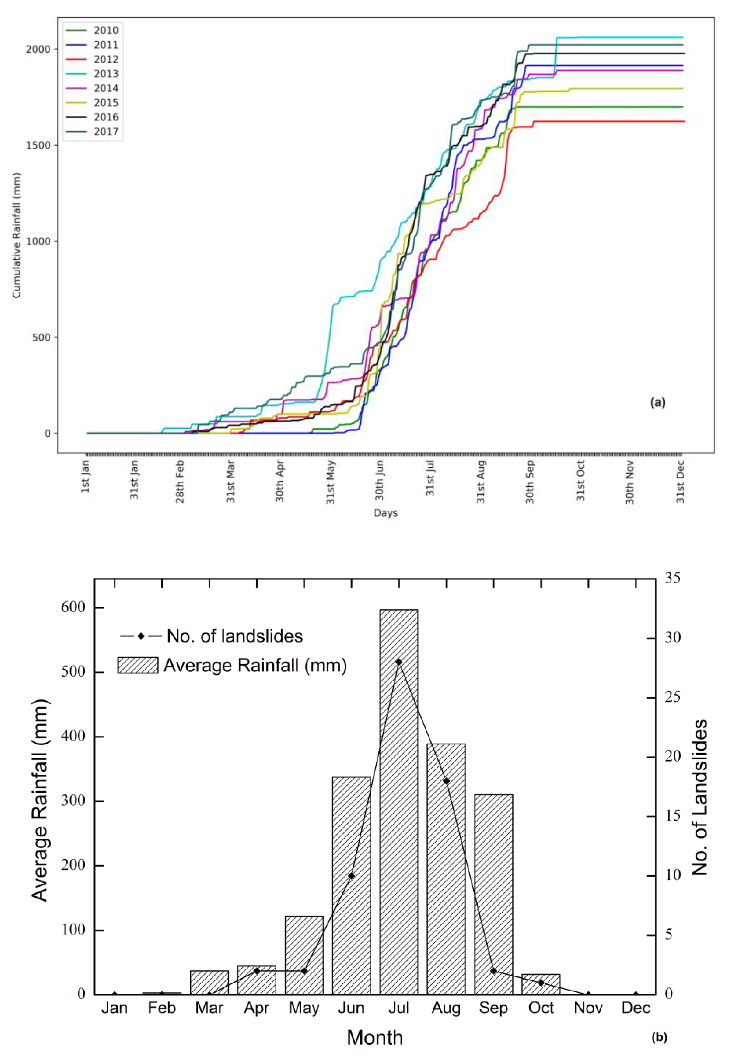
The annual cumulative rainfall for these years is plotted in
Figure 2a and the temporal distribution of landslides along with the average rainfall is shown in
Figure 2b. It is observed that the number of landslide events is maximum in the month of July where the rainfall peak is recorded. From
Figure 2b, it is clear that the number of landslides is directly related to the rainfall amount. Landslides are becoming an increasing menace in the region during monsoon season. The havocs related to landslides have multilevel impacts on the livelihood of population. Loss of farm lands and disruption of roads are affecting the income sources of the people. The socioeconomic development of the region is throttled by the disasters and associated setbacks. Hence, it is critical to adopt measures to minimize the impact of landslides in the region. An effective approach is to develop an early warning system using rainfall thresholds to forecast the occurrence of landslides. Since the area is affected by landslides of mixed typology (rapid shallow slides and slow deep seated movements), we took into account the SIGMA model [
23], specifically conceived for similar settings, and we customized it for an application in the study area.
3. The SIGMA Model
The SIGMA model was developed for the Emilia-Romagna region in Italy [
23]. This model uses the standard deviation of a statistical distribution as the key parameter for the analysis and defines thresholds as a function of standard deviation, predicting the potential of rainfall to initiate landslide events in the study area. Since the model is based on statistical distribution, it is easily exportable to other regions [
23]. Adopting the methodology from Martelloni et al. (2012) [
23], a customized SIGMA model for Kalimpong town is derived in this study. The modifications are in accordance with the historical database collected for the study area, thus making SIGMA compatible for a different hydro-meteo-geological setting than the area for which it is originally developed. The daily precipitation data were added at ‘
n’ days, with an ‘
n’ day wide shifting window which moves at everyday time steps throughout rainfall data. The values of ‘
n’ will vary from 1 to 365. To calculate the cumulative probability distribution for each data set, a standard distribution, which is the target function is chosen as a model [
34].This transformation relates the cumulative rainfall (z) with the target distribution (y = a,σ) (‘σ’ is the standard deviation of the series and ‘a’ is a multiplication constant). For each ‘
n’ day cumulative rainfall series, the values are sorted in ascending order such that
and a cumulative sample frequency is defined as
where,
The conversion is carried out using the cumulative distribution function of z, termed as F(z). For each value of zk, F(zk) defines the probability that the variable z takes a value less than zk, where k varies between 1 to n.
The original data z transformed to y is obtained as:
After applying the transformation function, from a particular value of standard deviation or its multiple, cumulative sample frequency and precipitation can be calculated. The same procedure is repeated for all values of
n from 1 to 365 and precipitation curves (σ curves) are plotted. The probability curves derived are used as the input values in the algorithm. A level of warning is predicted for everyday based on the rainfall thresholds. Rainfall recordings were cumulated with one day time steps for a particular time interval. These values are compared with the precipitation curves, from shorter to longer time frames [
23]. In the case of shallow landslides, the analysis should focus on the immediate effect of rainfall: the cumulative rainfall values up to two days before the day of analysis is considered. The decisional algorithm used is given in Equation 4:
where, Δ = a,σ,
C1–3 is the vector indicating the cumulated rainfall at time t and
are the thresholds relative to number of days
n and Δ [
23]. In the case of slow movements, the algorithm ponders the effect of cumulative rainfall from 4 days up to 63 days [
23]. The condition for crossing the threshold is given by:
The definitions of vector C are kept the same and have been used in the study for the analysis. The analysis was carried out in the same method proposed by the developers of the SIGMA model, to define the thresholds for Kalimpong town.
4. Analysis
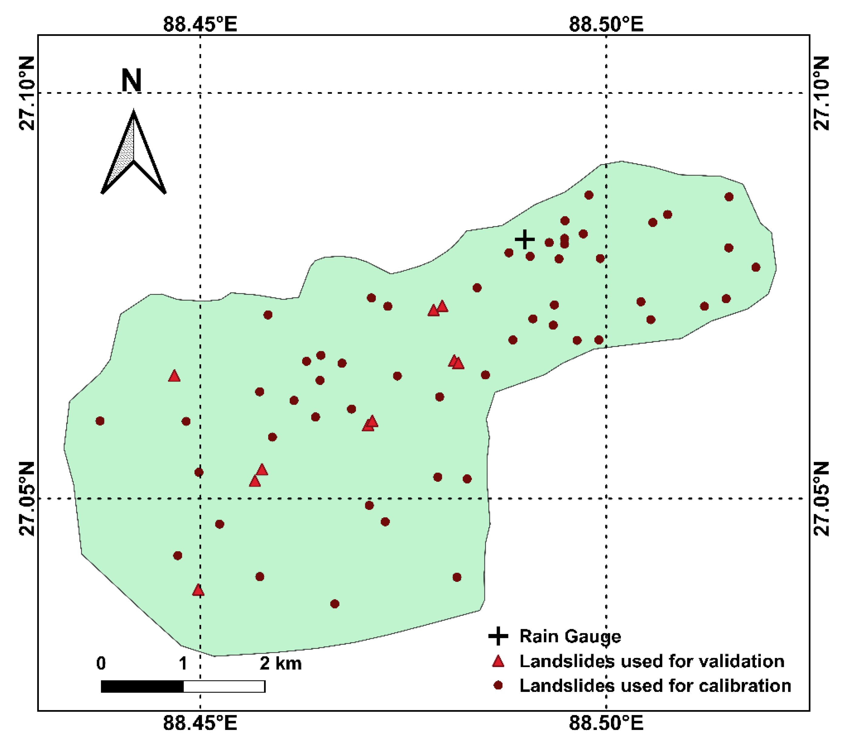
The rainfall and landslide data for Kalimpong town have been used to develop (2010–2015) and validate (2016 and 2017) rainfall thresholds for the region. The spatial distribution of landslide events during the study period is shown in
Figure 3.
For each day, ‘
n’-day cumulative rainfall values were calculated with
n ranging from 1 to 365. Cumulative probability distribution curves were plotted after sorting the values in ascending order. For small values of ‘
n’, the distributions were found to be closer to log-normal, and for higher values of ‘
n’, the distributions tend towards normal. The asymmetric distribution of data sets has been observed by other researchers as well [
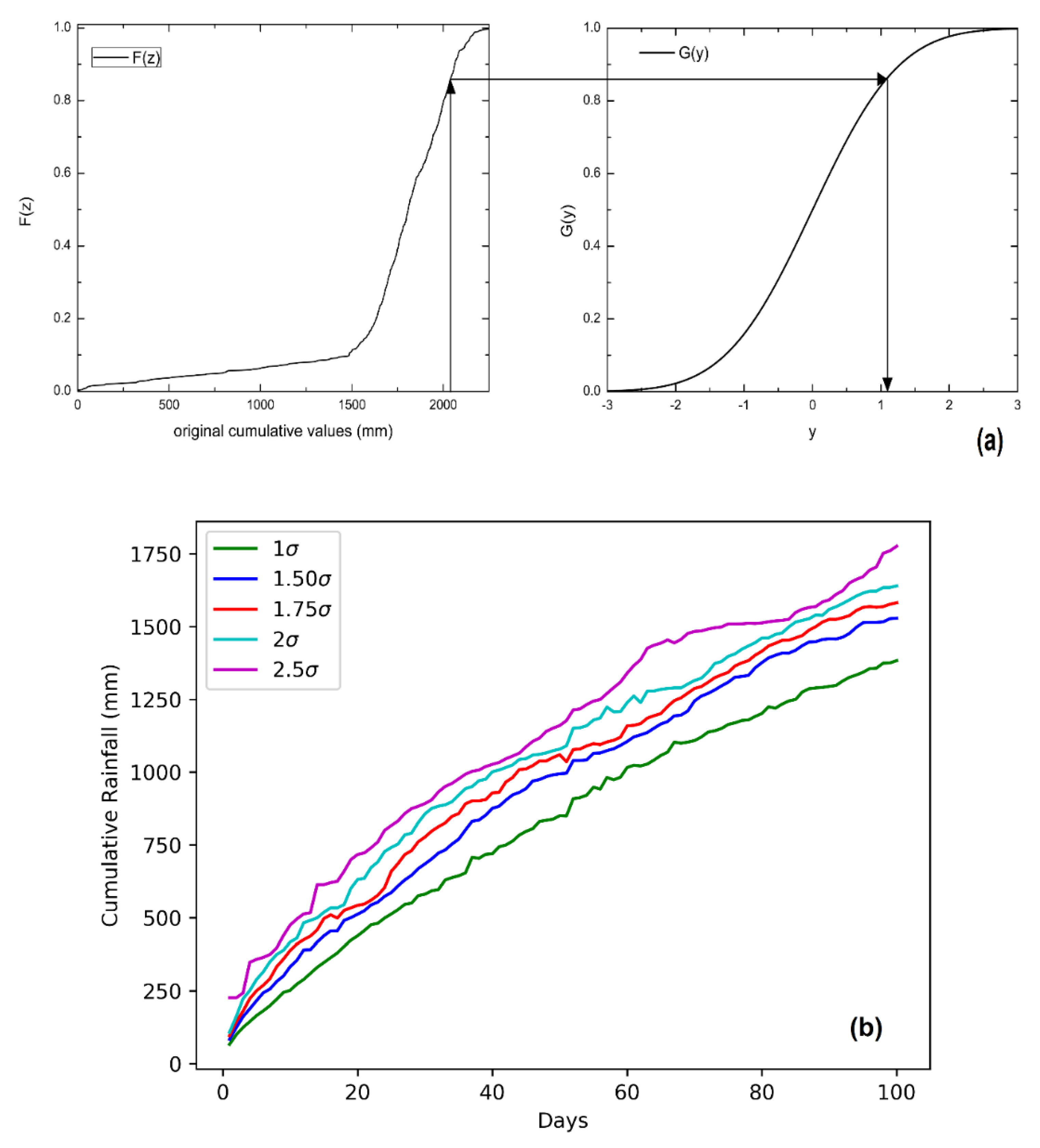
23]. Choosing Gaussian distribution as a target function, cumulative values corresponding to multiples of SIGMA were calculated by applying the transformation, as shown in
Figure 4a.
After applying the transformation, a probability of not overcoming a particular ‘aσ’ value can be calculated using the reverse procedure. For each value of ‘aσ’, cumulative values for
n-days varying from 1 to 365 were plotted as SIGMA curves. The values of standard curves were initially taken as 1.5σ, 1.75σ, 2σ and 2.5σ and are plotted in
Figure 4b.
From the probability distribution plots, SIGMA curves have been combined using an algorithm, which is the crucial part of the SIGMA model. The algorithm defines four different levels of alert, such as “red”, “orange”, “yellow” and “green”. These values are used to delineate exceptional rainfall values. The starting algorithm for the proposed model is as shown in
Figure 5. It considers the effect of short-term rainfall first, and exceedance of threshold will give high criticality alert for the day. If a red alert case does not exist, first orange alert level and then yellow alert level were checked for each day. If the result is negative in all cases, absent criticality (green color) is defined for the day. Hence, if a landslide happens to continue for a number of days, an effective model should predict the corresponding warning level on each day. The block diagram proposed in
Figure 5 has to be considered as a starting point for the work, since it was then calibrated as described in the following paragraphs.
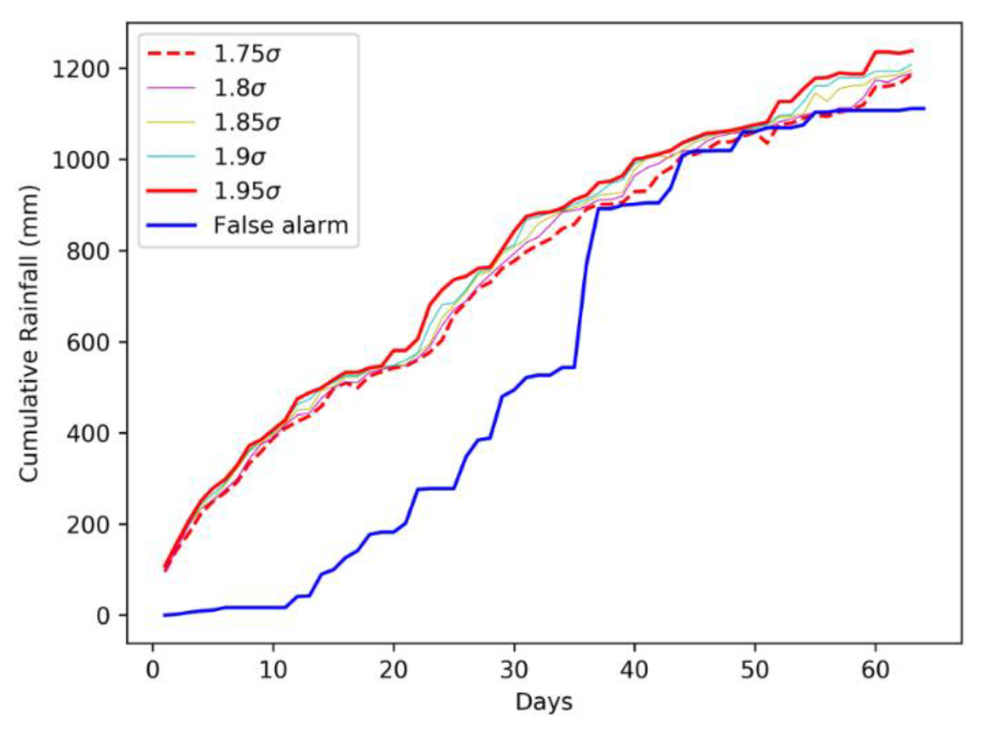
A threshold is considered to be exceeded if any of the elements in the vector crosses the value. Once a threshold is exceeded, the algorithm defines the level of warning on each day. These outputs were used to calibrate the model (data from 2010 to 2016). A trial and error procedure has been adopted in the optimization module of the algorithm, which relates the daily warning levels with landslide occurrences, as in Martelloni et al. (2012) [
23]. The value of threshold is progressively raised so that false alarms are avoided. A visualization of the procedure is shown in
Figure 6 where standard SIGMA value of 1.75 was optimized to 1.95. Using the same procedure, other standard values of 1.5 and 2 were optimized to 1.65, and 2.05, respectively. The standard value of 2.5 remained the same after optimization. The thresholds values were increased to minimize false alarms for each event, such that no true alarms are missed. The execution of this module terminates once the algorithm catches an event with an observed warning level conforming to the considered threshold. The standard SIGMA curves remain the same, but the calibration process gives a modified set of SIGMA curves for the region.
5. Results
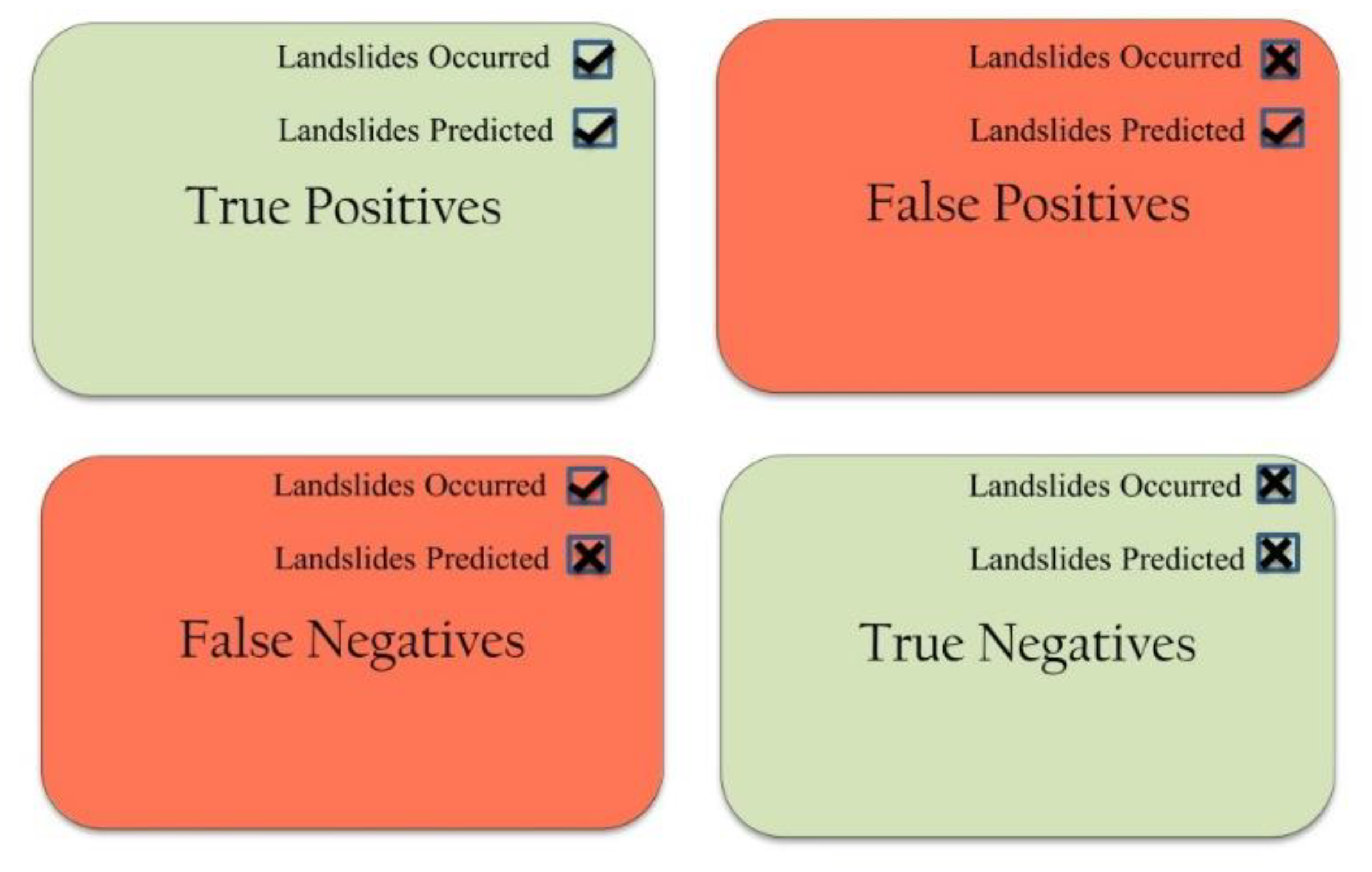
For the validation of results, rainfall and landslide data of 2016 and 2017 have been used. For each day of the validation period, the level of warning predicted by the decisional algorithm was compared with the reported landslide events according to the classical scheme of a confusion matrix, as shown in
Figure 7. A confusion matrix is used to describe the performance of a decisional algorithm on a validation dataset for which the true values are known. The performance of an algorithm can be visualized using this matrix.
Correct predictions can be both true positives (days in which the model forecasted correctly the occurrence of at least a landslide) and true negatives (days in which the model forecasted correctly that no landslides occurred). False negatives are those days in which the algorithm missed the alarms, and false positives are days in which the model issued false alarms. During 2016, eight shallow landslide events are reported in the region. The events were rapid in nature and happened to occur on a single day. Among the eight events, six were correctly predicted by the SIGMA model. Ground displacements were reported at two locations in the Chibo–Pashyor area during seven days in 2017: on 28th–29th July 2017 and 13th–17th August 2017 [
2]. In all seven days, ordinary criticality was well-predicted in the present analysis. 55 false alarms were forecasted in a span of two years. An overview of the quantitative validation of the model for Kalimpong is tabulated in
Table 2.
6. Discussion
The validation of the SIGMA model for the study area gave satisfactory results by predicting all slow movements events correctly and producing two missed alarms. However, this came at the cost of having a relatively high count of false alarms (22).
As pointed out by Lagomarsino et al. (2015) [
27], the most complete form of validation for a threshold model is to compare the skill scores to the ones obtained with the application of other models in the same test site. Several rainfall thresholds for landslides in Kalimpong region has already been defined [
2,
10,
15]. Therefore, the validation statistics of SIGMA were compared to those obtained in the same test site by two already published works, which make use of ED and ID thresholds, as shown in
Table 3.
It can be seen that during the validation period, SIGMA outperforms the other models. The terms for evaluating the overall performance of model, efficiency and likelihood ratio, are maximum for SIGMA among the models tested. Efficiency being the ratio of true predictions to a total number of predictions, does not show a significant variation amongst different models. This is often reported in LEWS [
27] where the number of true negatives are of a higher order than the other three variables. Specificity measures the ratio of correctly predicted days with no landslides to the total number of days without landslides, and sensitivity denotes the ratio of correctly predicted landslides to the total number of landslides. Likelihood ratio is the ratio of sensitivity to 1-specificity, evaluating the effect of both the parameters. The main reason for the better performance of SIGMA seems to be the effectiveness in predicting the slow movements occurred in 2017: a technique based on detecting antecedent rainfall anomalies. SIGMA is more suited than ID and ED thresholds to forecast slope movements with a complex hydrological response [
26]. ID and ED thresholds correctly predicted seven out of eight shallow landslides happened in 2016 but failed to forecast the slow movements in 2017 except for one day. It is also observed that the number of false alarms is also less in the SIGMA model, when compared with the other models. However, before having a definitive response on which would be the threshold model more effective to use in an EWS in Kalimpong, further tests are needed and a larger validation dataset needs to be accounted for.
In addition, the validation showed that SIGMA could need to be improved further, especially concerning the high number of false alarms. That was not a surprising outcome since in the calibration, the optimization procedure aimed at minimizing false negatives (missed alarms) instead of searching for a compromise between missed alarms and correct predictions, thus leading to a high number of false positives. A research direction worth exploring is testing different time intervals in the decisional algorithm: the one used in this research are the one resulted optimal for the Emilia-Romagna region (Italy), and they were defined after a long period of adjustments [
26]. The different physical settings of Kalimpong allow for a different optimal set of SIGMA values and time intervals to be defined.
7. Conclusions
Forecasting of rainfall-induced landslides in Kalimpong town have been carried out using the SIGMA model and considering the historical rainfall and landslide information. A single parameter, the cumulative rainfall, defines the threshold by means of a set of statistical thresholds.
The algorithm was designed to consider a three day rainfall effect for shallow landslides and more days (up to 63) for slow landslides. The time period and standard SIGMA values were decided by trial and error procedure during calibration, minimizing missed alarms and false alarms. A validation procedure showed satisfactory results and proved that SIGMA performed better than other ED and ID thresholds defined for the same region by previous works. For the study area, where both rapid and slow movements are present, the combined use of short-term and long-term antecedent rainfall is thus a point of strength of the model.
It can be concluded that the SIGMA model is a simple and efficient tool which can be used for landslide early warning on regional scale. The model predicts warning levels associated with each day, which can be directly linked to the severity of landslide events predicted. This study proves that the SIGMA model can be exported in parts of the world other than Italy, where the model was originally conceived, with satisfactory performance.
While applying the SIGMA model for a study area different from Italy, in a different hydro-meteo-geological setting, it was found that the values of
of Kalimpong is different from those used for Italy [
23]. A simpler algorithm than the one used for Italy was found to provide optimum results, as a smaller area and single rain gauge is considered for the analysis. Being a statistical model, the starting algorithm was decided by trial and error using the meteorological data and was fine-tuned by minimizing false alarms using an optimization procedure. The algorithm correctly predicted warnings on 13 out of 15 days of landslides during the validation period (2016–2017). The events in 2017 were the result of continuous rainfall over a longer time period. It can be concluded that this algorithm-based approach considers the effect of both long-term and short-term rainfall and even slow movements are predicted, providing a performance better than traditional ID and ED thresholds.
The number of false alarms generated has to be reduced either by tuning the SIGMA levels and the time interval lengths, or by improving the model conceptually. As an instance, physical parameters like soil moisture can be considered along with the rainfall data to increase the positive predictive power [
18,
25]. Also to expand the model for a larger area, spatial variability of meteorological parameters should be considered [
36,
37]. After further tests and developing standard action plans for each level of warning, this model has the potential to be integrated with rainfall forecasting and to be used as a landslide early warning system on a regional scale.
Author Contributions
Conceptualization, M.T.A. and N.S.; data curation, S.K.; formal analysis, M.T.A. and S.K.; methodology, S.S.; supervision, N.S., B.P. and S.S.; validation, M.T.A.; writing—original draft, M.T.A. and A.R.; writing—review and editing, N.S., B.P. and S.S. All authors have read and agreed to the published version of the manuscript.
Funding
The work has been carried out with the financial support of Department of Science & Technology (DST), New Delhi, for funding the research project Grant No. (NRDMS/02/31/015(G)); Florence University, in the framework of the project SEGONISAMUELERICATEN20.
Acknowledgments
The authors express our sincere gratitude to both the funding agencies. We are also thankful to Praful Rao and Save the Hills organization for their constant support throughout the study.
Conflicts of Interest
The authors declare no conflicts of interest.
References
- Froude, M.J.; Petley, D.N. Global fatal landslide occurrence from 2004 to 2016. Nat. Hazards Earth Syst. Sci. 2018, 18, 2161–2181. [Google Scholar] [CrossRef] [Green Version]
- Dikshit, A.; Satyam, N. Probabilistic rainfall thresholds in Chibo, India: Estimation and validation using monitoring system. J. Mt. Sci. 2019, 16, 870–883. [Google Scholar] [CrossRef]
- Van Westen, C.J.; Ghosh, S.; Jaiswal, P.; Martha, T.R.; Kuriakose, S.L. From landslide inventories to landslide risk assessment; an attempt to support methodological development in India. In Landslide Science and Practice; Springer: Berlin/Heidelberg, Germany, 2013; Volume 1, pp. 3–20. [Google Scholar]
- Piciullo, L.; Calvello, M.; Cepeda, J.M. Territorial early warning systems for rainfall-induced landslides. Earth-Science Rev. 2018, 179, 228–247. [Google Scholar] [CrossRef]
- Segoni, S.; Piciullo, L.; Gariano, S.L. A review of the recent literature on rainfall thresholds for landslide occurrence. Landslides 2018, 15, 1483–1501. [Google Scholar] [CrossRef]
- Caine, N. The rainfall intensity-duration control of shallow landslides and debris flows: An update. Geogr. Ann. Ser. A Phys. Geogr. 1980, 62, 23–27. [Google Scholar]
- Aleotti, P. A warning system for rainfall-induced shallow failures. Eng. Geol. 2004, 73, 247–265. [Google Scholar] [CrossRef]
- Guzzetti, F.; Peruccacci, S.; Rossi, M.; Stark, C.P. Rainfall thresholds for the initiation of landslides in central and southern Europe. Meteorol. Atmos. Phys. 2007, 98, 239–267. [Google Scholar] [CrossRef]
- Brunetti, M.T.; Peruccacci, S.; Rossi, M.; Luciani, S.; Valigi, D.; Guzzetti, F. Rainfall thresholds for the possible occurrence of landslides in Italy. Nat. Hazards Earth Syst. Sci. 2010, 10, 447–458. [Google Scholar] [CrossRef]
- Dikshit, A.; Satyam, D.N. Estimation of rainfall thresholds for landslide occurrences in Kalimpong, India. Innov. Infrastruct. Solut. 2018, 3, 24. [Google Scholar] [CrossRef]
- Rosi, A.; Peternel, T.; Jemec-Auflič, M.; Komac, M.; Segoni, S.; Casagli, N. Rainfall thresholds for rainfall-induced landslides in Slovenia. Landslides 2016, 13, 1571–1577. [Google Scholar] [CrossRef]
- Abraham, M.T.; Satyam, N.; Rosi, A.; Pradhan, B.; Segoni, S. The Selection of Rain Gauges and Rainfall Parameters in Estimating Intensity-Duration Thresholds for Landslide Occurrence: Case Study from Wayanad (India). Water 2020, 12, 1000. [Google Scholar] [CrossRef] [Green Version]
- Abraham, M.T.; Pothuraju, D.; Satyam, N. Rainfall Thresholds for Prediction of Landslides in Idukki, India: An Empirical Approach. Water 2019, 11, 2113. [Google Scholar] [CrossRef] [Green Version]
- Zhao, B.; Dai, Q.; Han, D.; Dai, H.; Mao, J.; Zhuo, L. Probabilistic thresholds for landslides warning by integrating soil moisture conditions with rainfall thresholds. J. Hydrol. 2019, 574, 276–287. [Google Scholar] [CrossRef]
- Teja, T.S.; Dikshit, A.; Satyam, N. Determination of Rainfall Thresholds for Landslide Prediction Using an Algorithm-Based Approach: Case Study in the Darjeeling Himalayas, India. Geosciences 2019, 9, 302. [Google Scholar] [CrossRef] [Green Version]
- Melillo, M.; Brunetti, M.T.; Peruccacci, S.; Gariano, S.L.; Roccati, A.; Guzzetti, F. A tool for the automatic calculation of rainfall thresholds for landslide occurrence. Environ. Model. Softw. 2018, 105, 230–243. [Google Scholar] [CrossRef]
- Peruccacci, S.; Brunetti, M.T.; Luciani, S.; Vennari, C.; Guzzetti, F. Lithological and seasonal control on rainfall thresholds for the possible initiation of landslides in central Italy. Geomorphology 2012, 139–140, 79–90. [Google Scholar] [CrossRef]
- Abraham, M.T.; Satyam, N.; Pradhan, B.; Alamri, A.M. Forecasting of Landslides Using Rainfall Severity and Soil Wetness: A Probabilistic Approach for Darjeeling Himalayas. Water 2020, 12, 804. [Google Scholar] [CrossRef] [Green Version]
- Lagomarsino, D.; Segoni, S.; Fanti, R.; Catani, F. Updating and tuning a regional-scale landslide early warning system. Landslides 2013, 10, 91–97. [Google Scholar] [CrossRef]
- Bai, S.; Wang, J.; Thiebes, B.; Cheng, C.; Yang, Y. Analysis of the relationship of landslide occurrence with rainfall: A case study of Wudu County, China. Arab. J. Geosci. 2014, 7, 1277–1285. [Google Scholar] [CrossRef]
- Lee, M.L.; Ng, K.Y.; Huang, Y.F.; Li, W.C. Rainfall-induced landslides in Hulu Kelang area, Malaysia. Nat. Hazards 2014, 70, 353–375. [Google Scholar] [CrossRef]
- Althuwaynee, O.F.; Pradhan, B.; Ahmad, N. Estimation of rainfall threshold and its use in landslide hazard mapping of Kuala Lumpur metropolitan and surrounding areas. Landslides 2015, 12, 861–875. [Google Scholar] [CrossRef]
- Martelloni, G.; Segoni, S.; Fanti, R.; Catani, F. Rainfall thresholds for the forecasting of landslide occurrence at regional scale. Landslides 2012, 9, 485–495. [Google Scholar] [CrossRef] [Green Version]
- Crosta, G. Regionalization of rainfall thresholds: An aid to landslide hazard evaluation. Environ. Geol. 1998, 35, 131–145. [Google Scholar] [CrossRef]
- Segoni, S.; Rosi, A.; Lagomarsino, D.; Fanti, R.; Casagli, N. Brief communication: Using averaged soil moisture estimates to improve the performances of a regional-scale landslide early warning system. Nat. Hazards Earth Syst. Sci. 2018, 18, 807–812. [Google Scholar] [CrossRef] [Green Version]
- Segoni, S.; Rosi, A.; Fanti, R.; Gallucci, A.; Monni, A.; Casagli, N. A regional-scale landslide warning system based on 20 years of operational experience. Water 2018, 10, 1297. [Google Scholar] [CrossRef] [Green Version]
- Lagomarsino, D.; Segoni, S.; Rosi, A.; Rossi, G.; Battistini, A.; Catani, F.; Casagli, N. Quantitative comparison between two different methodologies to define rainfall thresholds for landslide forecasting. Nat. Hazards Earth Syst. Sci. 2015, 15, 2413–2423. [Google Scholar] [CrossRef] [Green Version]
- Wadia, D.N. Geology of India; Tata McGrawHill: New Delhi, India, 1975. [Google Scholar]
- Sumantra, S. Causes of Landslides in Darjeeling Himalayas during June-July, 2015. J. Geogr. Nat. Disasters 2016, 6. [Google Scholar] [CrossRef] [Green Version]
- Mukherjee, A.; Mitra, A. Geotechnical Study of Mass Movements Along the Kalimpong Approach Road in the Eastern Himalayas. Indian J. Geol. 2001, 73, 271–279. [Google Scholar]
- CartoDEM. Available online: https://bhuvan-app3.nrsc.gov.in/data/download/index.php (accessed on 20 August 2019).
- Save The Hills Blog. Available online: http://savethehills.blogspot.com/ (accessed on 3 December 2019).
- Dikshit, A.; Satyam, D.N.; Towhata, I. Early warning system using tilt sensors in Chibo, Kalimpong, Darjeeling Himalayas, India. Nat. Hazards 2018, 94, 727–741. [Google Scholar] [CrossRef]
- Goovaerts, P. Geostatistics for Natural Resources Evaluation; Oxford University Press: Oxford, UK, 1997. [Google Scholar]
- Dikshit, A.; Satyam, N. Rainfall Thresholds for the prediction of Landslides using Empirical Methods in Kalimpong, Darjeeling, India. In Proceedings of the JTC1 Workshop on Advances in Landslide Understanding, Barcelona, Spain, 24–26 May 2017. [Google Scholar]
- Lu, B.; Charlton, M.; Harris, P.; Fotheringham, A.S. Geographically weighted regression with a non-Euclidean distance metric: A case study using hedonic house price data. Int. J. Geogr. Inf. Sci. 2014, 28, 660–681. [Google Scholar] [CrossRef]
- Pasculli, A.; Palermi, S.; Sarra, A.; Piacentini, T.; Miccadei, E. A modelling methodology for the analysis of radon potential based on environmental geology and geographically weighted regression. Environ. Model. Softw. 2014, 54, 165–181. [Google Scholar] [CrossRef]
© 2020 by the authors. Licensee MDPI, Basel, Switzerland. This article is an open access article distributed under the terms and conditions of the Creative Commons Attribution (CC BY) license (http://creativecommons.org/licenses/by/4.0/).

