Article

Calibration of a Distributed Hydrological Model in a Data-Scarce Basin Based on GLEAM Datasets

1
School of Geographical Science, Qinghai Normal University; Key Laboratory of Physical Geography and Environmental Processes; MOE Key Laboratory of Tibetan Plateau Land Surface Processes and Ecological Conservation, Xining 810016, China
2
Academy of Plateau Science and Sustainability, Xining 810016, China
*
Author to whom correspondence should be addressed.
Water 2020, 12(3), 897; https://doi.org/10.3390/w12030897
Submission received: 12 February 2020 / Revised: 18 March 2020 / Accepted: 19 March 2020 / Published: 22 March 2020
(This article belongs to the Special Issue Advanced Hydrologic Modeling in Watershed-Scale)

Abstract

:
The calibration of hydrological models is often complex in regions with scarce data, and generally only uses site-based streamflow data. However, this approach will yield highly generalised values for all model parameters and hydrological processes. It is therefore necessary to obtain more spatially heterogeneous observation data (e.g., satellite-based evapotranspiration (ET)) to calibrate such hydrological models. Here, soil and water assessment tool (SWAT) models were built to evaluate the advantages of using ET data derived from the Global Land surface Evaporation Amsterdam Methodology (GLEAM) to calibrate the models for the Bayinhe River basin in northwest China, which is a typical data-scarce basin. The result revealed the following: (1) A great effort was required to calibrate the SWAT models for the study area to obtain an improved model performance. (2) The SWAT model performance for simulating the streamflow and water balance was reliable when calibrated with streamflow only, but this method of calibration grouped the hydrological processes together and caused an equifinality issue. (3) The combination of the streamflow and GLEAM-based ET data for calibrating the SWAT model improved the model performance for simulating the streamflow and water balance. However, the equifinality issue remained at the hydrologic response unit (HRU) level.
Keywords:
SWAT; GLEAM; ET; streamflow

1. Introduction

Distributed hydrological models are important tools for revealing the hydrological processes that occur in a changing environment [1]. However, a hydrological model includes multiple complex parameters. Hence, various inputs are required to accurately simulate hydrological processes [2]. Although less effort is needed to calibrate a hydrological model if the input data are reliable and comprehensive [3], in some regions with data scarce, the calibration of a hydrological model is complex and requires considerable effort. Recently, auto-calibration software and methods for hydrological models have been developed, for example, Parameter ESTimation (PEST) [4], the Shuffled Complex Evolution algorithm (SCE-UA) [5], and SWAT Calibration Uncertainty Programs (SWAT-CUP) [6]. These tools are convenient for model calibration; however, there is more than one set of optimal parameters after a calibration using auto-calibration software or methods [7,8]. Moreover, although some of the parameters are reasonable, others are not, and it is difficult to evaluate whether the calibrated parameters are correct. The main output variables of a hydrological model are streamflow, evapotranspiration (ET), soil water content, surface runoff, groundwater flow, and lateral flow [7,9]. However, generally, only site-based streamflow data are used to calibrate and validate a hydrological model because it is difficult to observe other variables [9]. Furthermore, in some watersheds, there are only a few hydrological stations that are heterogeneously distributed. As a result, an auto-calibrated model using site-based streamflow data will yield highly generalised values for all model parameters and hydrological processes of the watershed [10,11]. Therefore, to obtain reasonable model parameters and to better simulate watershed hydrological processes, it is necessary to combine the model auto-calibration procedure with both site-based streamflow and other spatially heterogeneous observation data.
ET is one of the most important components of the water balance; approximately 60–70% of precipitation returns to the atmosphere from the land surface. The remaining precipitation may become streamflow or enter other forms of water. With the development of remote sensing, ET data are no longer difficult to obtain. With the help of remote sensing technology, energy data relating to the soil–vegetation–air interface can be extracted, and then combined with site-based meteorological data to calculate the regional ET based on the traditional algorithm. Many regional ET models exist, including the Reg model [4], Priestley–Taylor jet propulsion laboratory model (PT-JPL) [12], Penman–Monteith MODIS global terrestrial evapotranspiration algorithm (PM-MOD16) [13], and Global Land surface Evaporation Amsterdam Methodology (GLEAM) [14] amongst others.
Due to the different structures of datasets, models perform differently in terms of ET simulation. Models have been validated with observed data and have been reported to perform well in most places in China [15]. Therefore, most datasets can be used directly to calibrate and validate hydrological models. Immerzeel and Droogers [16] incorporated remote sensing-derived ET data (based on MODIS data and the SEBAL model) into their calibration of the Soil and water assessment tool (SWAT) for a catchment in the Krishna basin in southern India. After calibration, the performance of the SWAT to simulate ET showed an obvious increase. Rientjes et al. [17] used streamflow and satellite-based actual ET (based on MODIS data and the SEBAL model) to calibrate the HBV rainfall-runoff model for the Karkheh River basin in Iran. The authors concluded that the catchment water balance was best reproduced when both streamflow and satellite-based ET served as the calibration target. Parajuli et al. [18] applied time series PM-MOD16 ET data to evaluate the SWAT calibration. They demonstrated the use of satellite-based ET data to evaluate the SWAT performance, which can be applied in watersheds with a lack of meteorological data. In these studies, satellite-based ET data were used to optimise the hydrological model parameters, and the simulated results of the actual ET or streamflow were good. However, many satellite-based ET datasets are missing data for most places in northwest China [15].
GLEAM is a series of algorithms to calculate the components of surface ET based on remote sensing data for water and heat [14]. Compared with other surface ET datasets, GLEAM can not only effectively distinguish soil evaporation, plant emission, plant interception evaporation, snow evaporation, water surface evaporation and other components involved in the process of surface ET, but also considers radiation, temperature, precipitation and the surface layer in the calculation process [14]. In addition, GLEAM datasets perform well and cover the entire area of China [19], and can be directly used to calibrate and validate hydrological models.
Many inland rivers exist in northwest China, which generally originates in mountainous areas and dissipates in piedmont plain areas. The land-surface conditions, environment, and climate are therefore different in the upper, middle, and lower reaches. The best way to simulate the hydrological processes in these inland watersheds is to build individual models for each of these reaches [7,20]. However, there is often a lack of observational data (e.g., precipitation and streamflow) that are key for building hydrological models successfully. The Bayinhe River, located in the northeast Qaidam basin, is a typical inland river [21]. The upper reach of the Bayinhe River is situated in Qilian Mountain and the middle reach is in the Zelinggou basin and Delingha City. Only one hydrological station and one meteorological station exist in the entire watershed, both of which are in the middle reach. There is, therefore, an issue regarding how the hydrological processes can be simulated for this basin with data scarce.
The objective of this research is to evaluate the advantages of using the ET data derived from the GLEAM to separately calibrate the widely used SWAT model for the upper and middle reaches of the Bayinhe River. We combine actual streamflow data in one calibration as a means of simplifying the calibration process and improving the model performance.

2. Materials and Methods
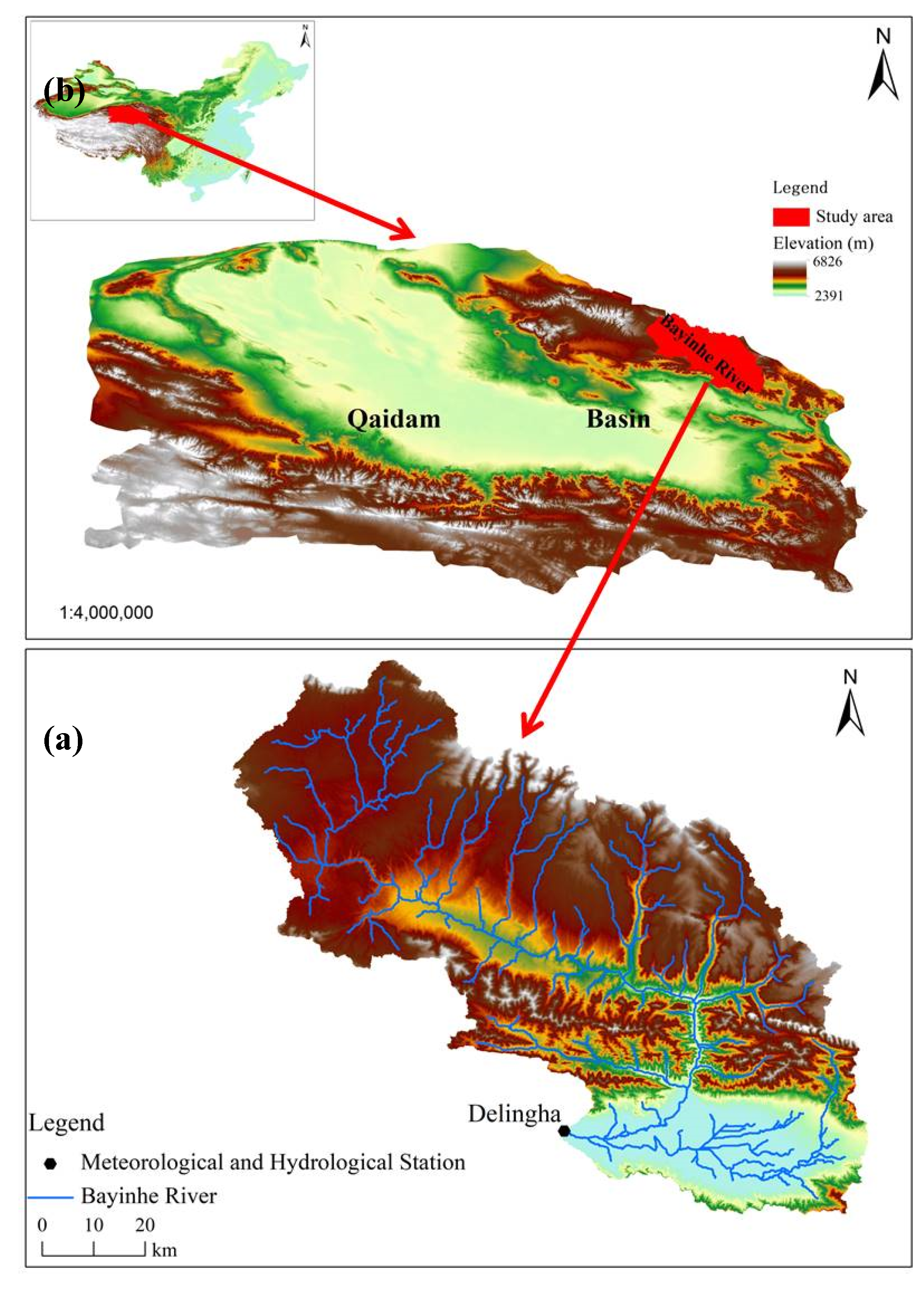
2.1. Study Area

The Bayinhe River basin is an archetypical, alpine inland river basin located at the north-eastern edge of the Qaidam basin. The river itself originates from the Zongwulong mountain range on the southern slopes of Mount Qilian (average elevation 4200 m). The river exits the mountains into the Zelinggou basin and then travels through the basin before flowing into Delingha City [21]. Finally, the river splits and flows east into Keluke Lake and west into Gahai Lake. According to statistics from the Delingha meteorological station, the mean annual precipitation in the Bayinhe River basin between 1999 and 2019 was 210 mm, and the mean annual temperature was 5.81 °C. The Bayinhe River basin is a typical ecologically fragile, arid and semi-arid plateau. The region’s primary land cover types are desert and grassland with primarily light frigid calcic soil and dark frigid calcic soil. This study takes the upper and middle reaches of the Bayinhe River basin (above the Delingha hydrological station) as its study area (Figure 1).

2.2. Data Preparation

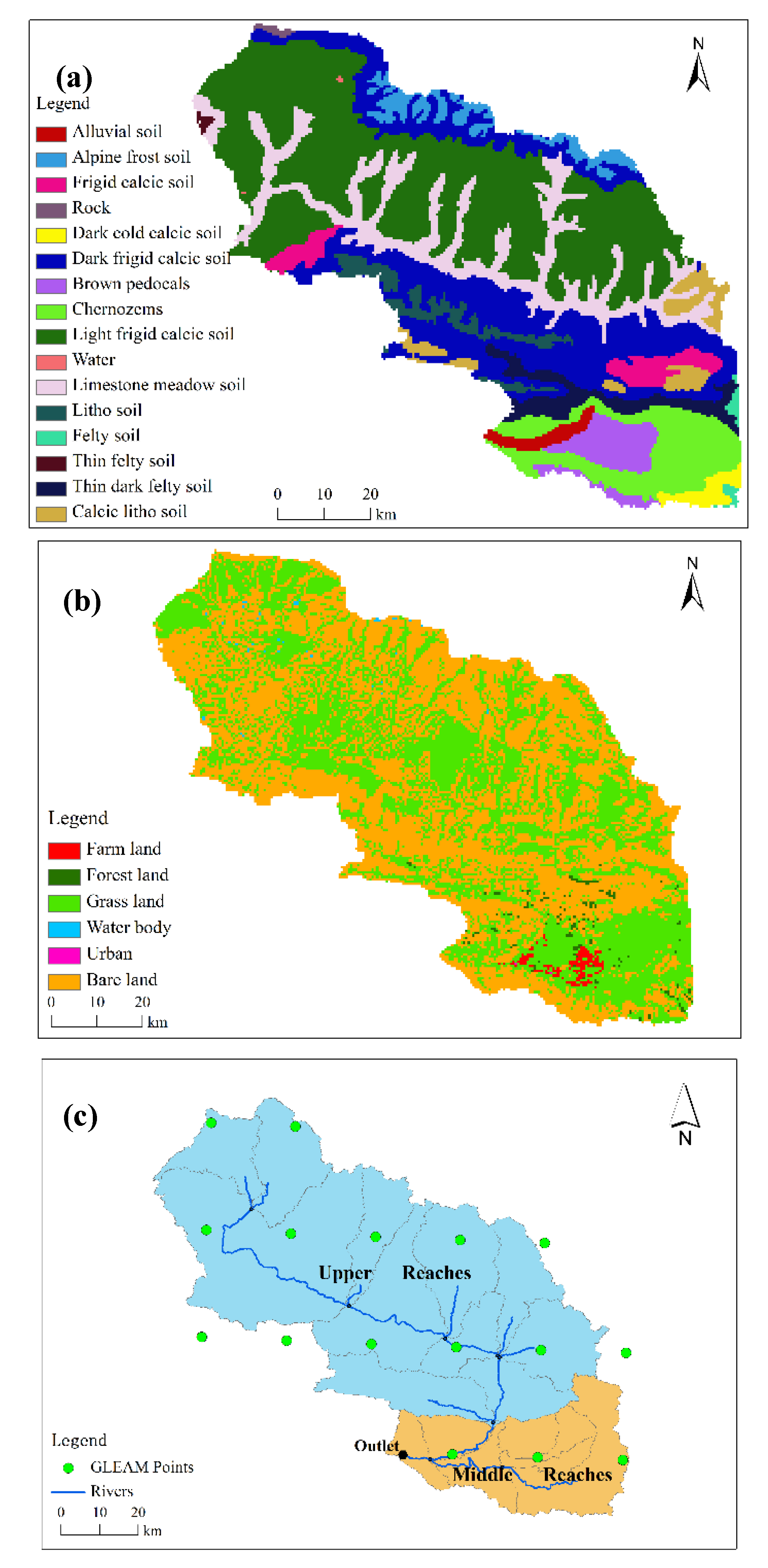
2.2.1. Basic Data of the SWAT Model

Setting up the surface parameters for a SWAT model requires soil data, land use data, topographic data, and a drainage basin outlet point. Soil classification data (Figure 2a) were taken from the 1:1,000,000 soil types from the dataset of Qinghai Province, while relevant soil hydrology data were referenced from the Soils of Qinghai Province. Land use data (Figure 2b) were cropped from the 1:100,000 China land use dataset for 2015. To correspond data to the land use types in the SWAT hydrological model database, land use types were reclassified as farmland, forest, grassland, water bodies, residential land, and bare land. Terrain data (Figure 1) had a 30 × 30 m resolution (ASTER GDEM). In addition, the Delingha hydrological station was selected as the basin’s outlet point. Figure 2c delineates the sub-basins that comprise the middle and upper reaches of the Bayinhe River basin. This study divided the region into a total of 17 sub-basins.

2.2.2. Data for Model Calibration

Two types of datasets were used to calibrate the SWAT model: (i) the monthly streamflow data from the Delingha hydrological station for 2006 to 2015, and (ii) the monthly actual ET in each sub-basin as derived from the GLEAM datasets for 2006 to 2015.
The GLEAM includes a series of algorithms to calculate the components of surface ET based on satellite data for water and heat (Table 1). The algorithms calculate the potential ET based on the Priestley–Taylor method [22]. There are four modules in the GLEAM to calculate the different proportions of the ET process: the interception model, soil water module, stress module and Priestley and Taylor model [14]. The GLEAM provides daily actual ET data at a 0.25° × 0.25° spatial resolution. Figure 3 illustrates the coverage of the GLEAM dataset for the study area.

2.3. SWAT Model

SWAT is a semi-distributed hydrologic model; it first uses a conceptual model to estimate precipitation, streamflow, and sediment for each individual hydrologic response unit (HRU). After these calculations are complete, the SWAT calculates the convergence of the river basin channels. Finally, the flow rate and sediment and pollutant loads for the basin outlet section are obtained [9].
The simulation of watershed hydrology by the SWAT can be divided into (1) the land-surface component of the water cycle (flow and slope convergence), which controls the input of water, sediment, and nutrients in the main channel of each sub-basin, and (2) the surface water component of the water cycle (channel convergence), which determines the transport of water, sediment, and other substances from the channel network to the basin outlet [9].
The water volume calculation of the SWAT model is based on the principle of water volume balance and follows Equation (1) [9]:
SWC t = SWC 0 + i = 1 t ( R day W surf E t SC seep W gw )
where SWC t is the soil water content (mm); SWC 0 is the soil water content in the previous period (mm); t is the model time step; R day is the amount of precipitation on i day (mm); W surf indicates the surface streamflow of the i-th day (mm); E t represents the actual ET (mm); SC seep represents the soil permeation of i-th day (mm); W gw represents the amount of basic flow (mm).

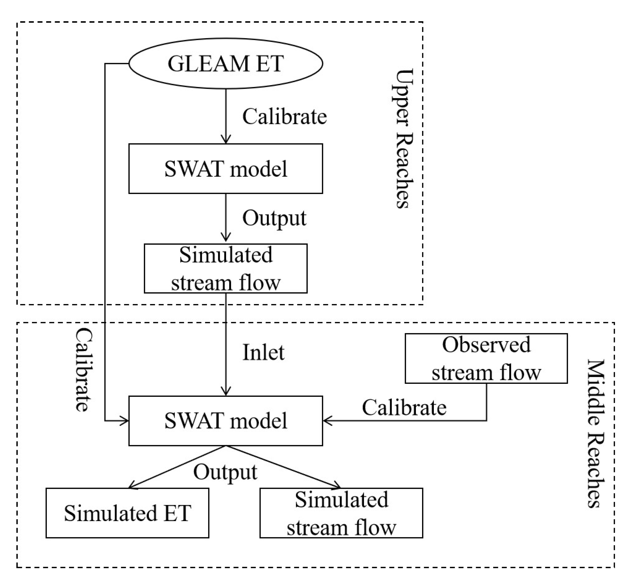
2.4. SWAT Model Calibration Strategy

Three SWAT models were built: (1) SWAT1 simulates the water balance of the entire study area (upper and middle reaches of the Bayinhe River), and is calibrated by the stream outflow from the middle reach; (2) SWAT2U simulates the water balance of the upper reach of the Bayinhe River and is calibrated with the GLEAM based ET data; (3) SWAT2M simulates the water balance of the middle reach of the Bayinhe River and is calibrated with the GLEAM-based ET data and stream outflow from the middle reach. For the SWAT2M, the simulated stream outflow from the upper reach was directly used as the inflow to the middle reach. The auto-calibration tool SWAT-CUP combined with a manual calibration strategy [9] were used to calibrate the SWAT model based on observed data. The Nash-Sutcliff efficiency (NSE), percent bias (PBIAS) and coefficient of determination (R2) were used to evaluate the performance of the three SWAT models.
Figure 3 shows the unique calibration strategy used in this study (SWAT2U and SWAT2M). Firstly, the upper and middle reaches were separately modelled. Secondly, the satellite-based ET data derived from the GLEAM dataset were used to calibrate the SWAT model to simulate the water balance of the upper reach of the Bayinhe River. Thirdly, the simulated stream outflow from the upper reach was used as the inflow to the middle reach. The ET data and streamflow data were then used to calibrate the SWAT model for the middle reach of the Bayinhe River.

2.5. Parameters Sensitivity

In this study, 25 model parameters related to ET and streamflow were selected and their sensitivities were calculated. The sequential uncertainty fitting (SUFI2) algorithm was combined with the global sensitivity method in SWAT-CUP software (Swiss Federal institute of Aquatic Science and Technology, Duebendorf, Swizerland) and used to evaluate parameter sensitivities. The SUFI2 algorithm in SWAT-CUP combined with the SWAT-CUP and manual calibration strategy [9] were used to calibrate the three SWAT models based on the parameter sensitivity results (Section 3.1).

2.6. Indicators for Evaluating the SWAT Model Simulation Result

Based on the results of [23], this study uses the NSE (Equation (2)), PBIAS (Equation (3)), and R2 (Equation (4)) to evaluate the performance of the SWAT model.
NSE = 1 i = 1 n ( S i o b s S i s i m ) 2 i = 1 n ( S i o b s S ¯ o b s ) 2
PBIAS = i = 1 n ( S i o b s S i s i m ) × 100 i = 1 n ( S i o b s )
R 2 = [ i = 1 N ( P i s i m P ¯ s i m ) ( P i o b s P ¯ o b s ) ] 2 i = 1 N ( P i s i m P ¯ s i m ) 2 i = 1 N ( P i o b s P ¯ o b s ) 2
In Equations (2)–(4), S i o b s represents the measured flow, S i s i m represents the simulated flow, and S ¯ o b s represents the mean of the measured flow. NSE values range from negative infinity to 1; the closer the value of NSE to 1, the better and more credible the simulation results are. The closer the value of NSE to 0.5, the closer the simulation results are to the observed values, which means that the overall model result is credible; however, the process simulation error is large. If the NSE is far less than 0, the model is not reliable. If the PBIAS value is between −10% and 10%, the model results are good. R 2 ranges from 0 to 1, whereby the closer the value of R 2 is to 1, the better and more credible the simulation results are [23].

3. Results

3.1. Parameters Sensitivity

Table 2 presents the results for the first ten sensitivity parameters of the SWAT1, SWAT2U, and SWAT2M models. The higher the absolute value of t-Stat and the lower the p-value, the more sensitive the parameter is. The first ten sensitivity parameters for the SWAT1 model were CN2 (the SCS runoff curve number), CH_K2 (the effective hydraulic conductivity in main-channel alluvium), SOL_BD (the moist bulk-density), CH_N2 (Manning’s “n” value for the main channel), SOL_K (the saturated hydraulic-conductivity), SOL_AWC (the available water capacity of the soil layer), GW_REVAP (a groundwater “revap” coefficient), GWQMN (the threshold depth of water in the shallow aquifer required for return flow to occur), SLSUBBSN (the average slope length), and SMFMN (the annual minimum melt-rate for snow). The first ten sensitivity parameters for the SWAT2U model were CN2, SOL_BD, SOL_K, ESCO (a soil evaporation compensation factor), SLSUBBSN, GWQMN, SMFMN, SNOCOVMN (a snow-pack temperature lag factor), SNO50COV (the fraction of the snow volume in a given area that corresponds to 50% of the snow cover) and CH_N2. The first ten sensitivity parameters for the SWAT2M model were CN2, SOL_BD, SLSUBBSN, SOL_K, HRU_SLP (the average slope steepness), ALPHA_BF (the baseflow alpha-factor), SOL_AWC, ESCO, GW_REVAP, and GWQMN. The first ten sensitivity parameters were different for the three SWAT models because different calibration data were used.

3.2. Non-Calibrated SWAT

The non-calibrated SWAT model results can demonstrate how well the SWAT model predicts the streamflow before calibration, which indicates the effort required for calibration when using each configuration [3]. Figure 4 exhibits the monthly streamflow at the outlet of the middle reach simulated by the non-calibrated SWAT. The performance of the non-calibrated SWAT was poor: R2 < 0.50, NSE < 0.50, and PBIAS < −20%. Moreover, the simulated and observed streamflow were not well matched in each year.

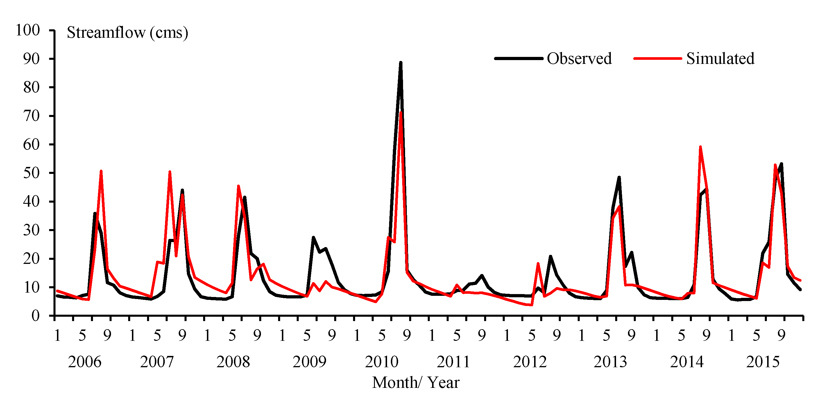
3.3. SWAT1 Performance

Figure 5 exhibits the monthly streamflow at the outlet of the middle reach simulated by the calibrated SWAT1 (R2 = 0.74; NSE = 0.73; PBIAS = 0.6%). Compared to the non-calibrated SWAT (R2 = 0.06; NSE = −0.11; PBIAS = −34.5%), the performance of the SWAT1 model to simulate the monthly streamflow improved by ~863.6% to 1133.3%. The simulated and observed streamflow were well matched except for some specific years (e.g., the fourth and sixth years) when the simulated streamflow was particularly low.

3.4. SWAT2U Performance

In the SWAT2U model, the ranges of some important and sensitive parameters (i.e., SMFMN, SNOCOVMN, SNO50COV, and ALPHA_BF) were assigned according to existing research for some similar watersheds [23,24]. Figure 6 shows the annual average ET simulated by the SWAT2U model for the upper reach of the Bayinhe River. In most of the sub-basins, the observed ET derived from the GLEAM was higher than that of the SWAT model. Table 3 presents the performance of the SWAT2U model for simulating the monthly ET in each sub-basin. All R2 values were >0.90, all NSE values were >0.84 and PBIAS values were within −20% to 20%. Hence, the SWAT2U model was well-calibrated by using the monthly ET data derived from the GLEAM. Figure 7 exhibits the simulated stream outflow from the upper reach. This part of the streamflow was the inflow for the middle reach.

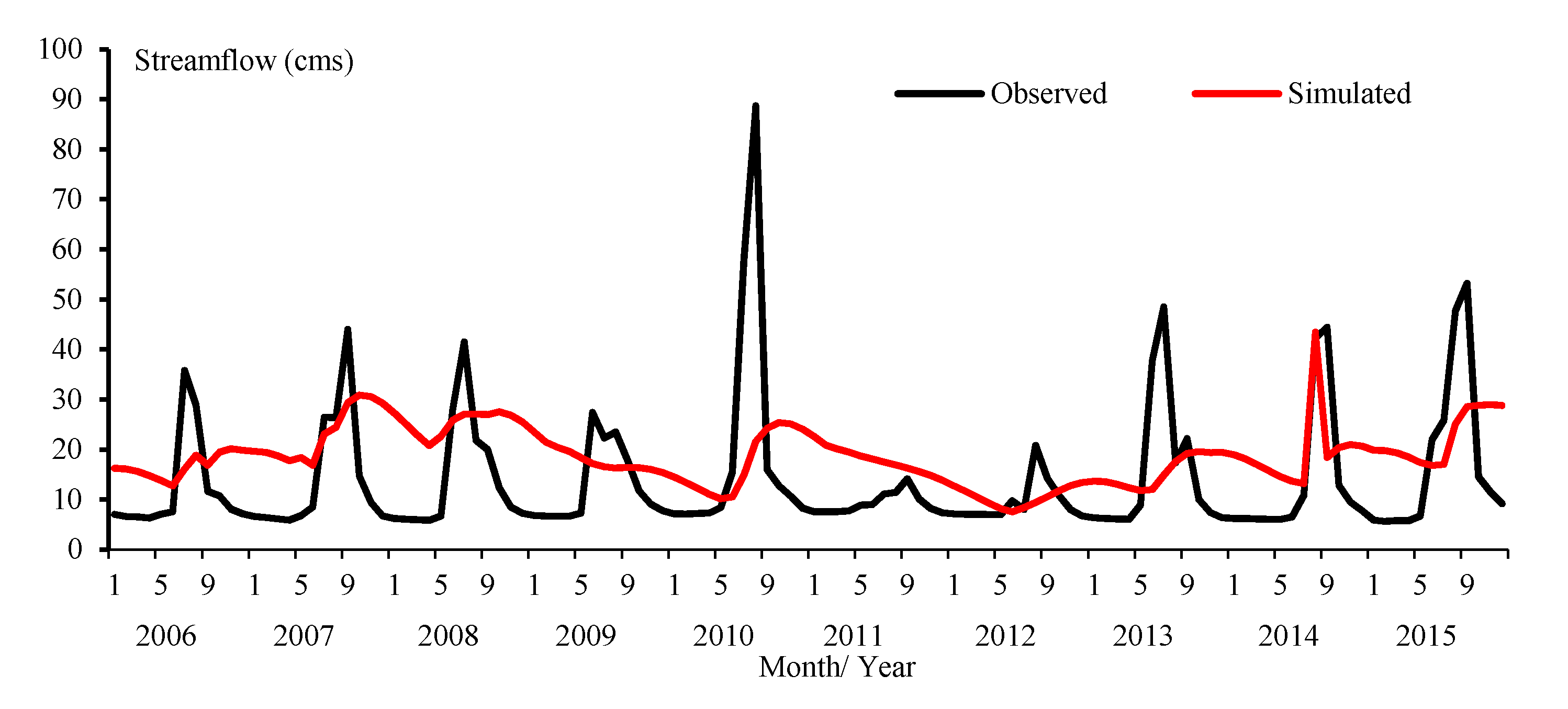
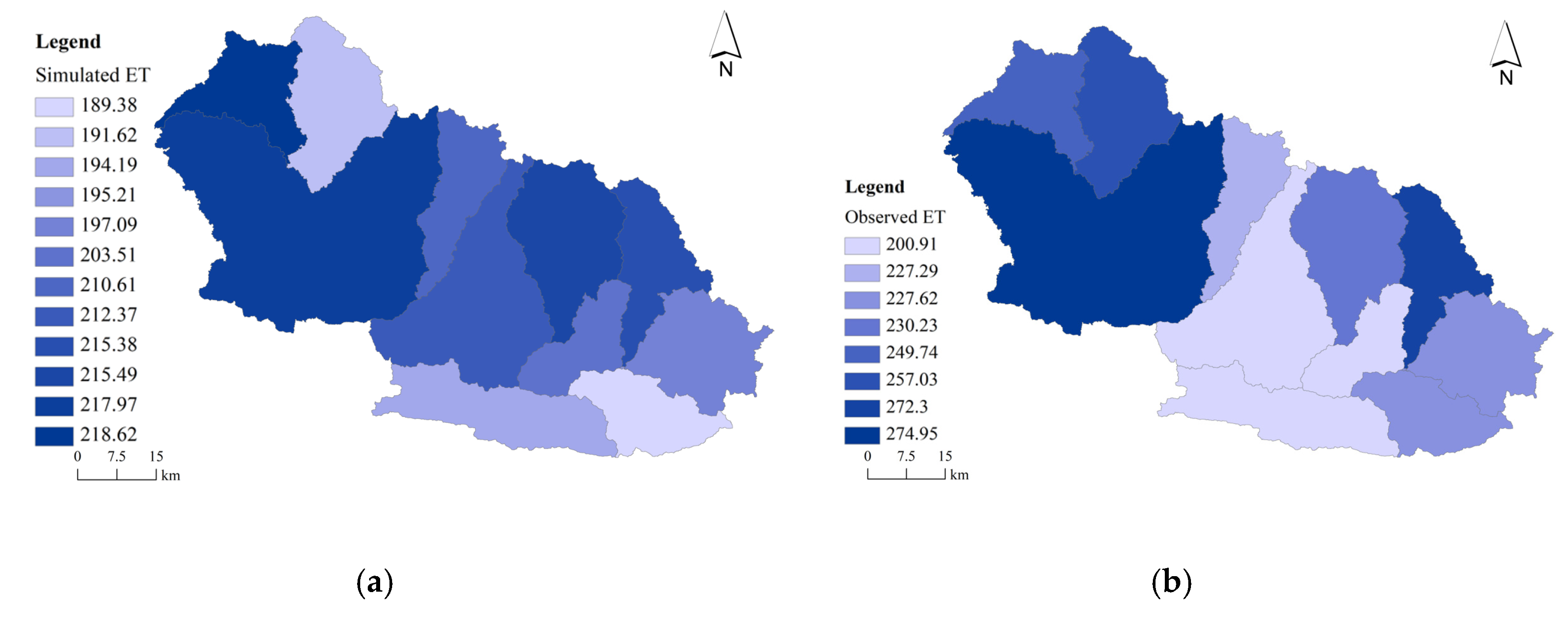
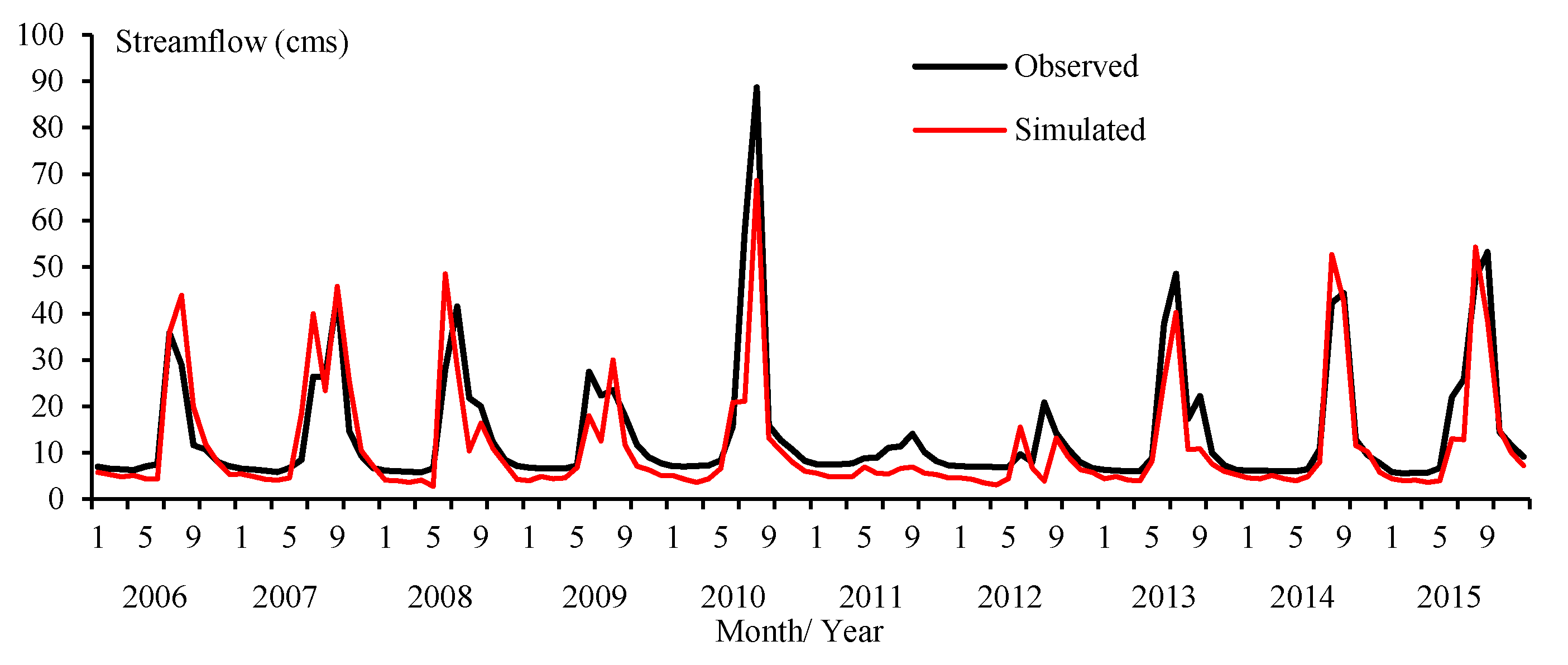
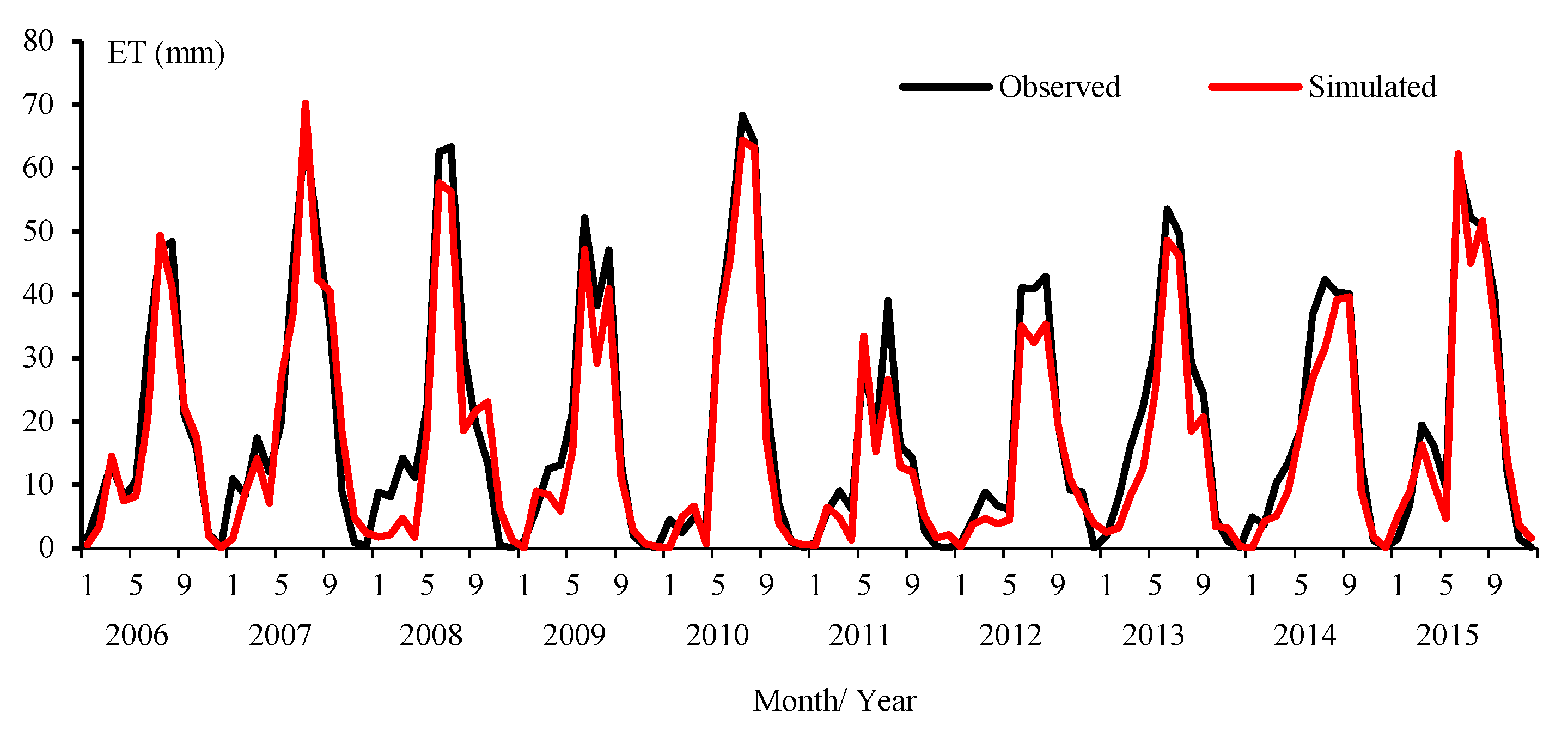
3.5. SWAT2M Performance
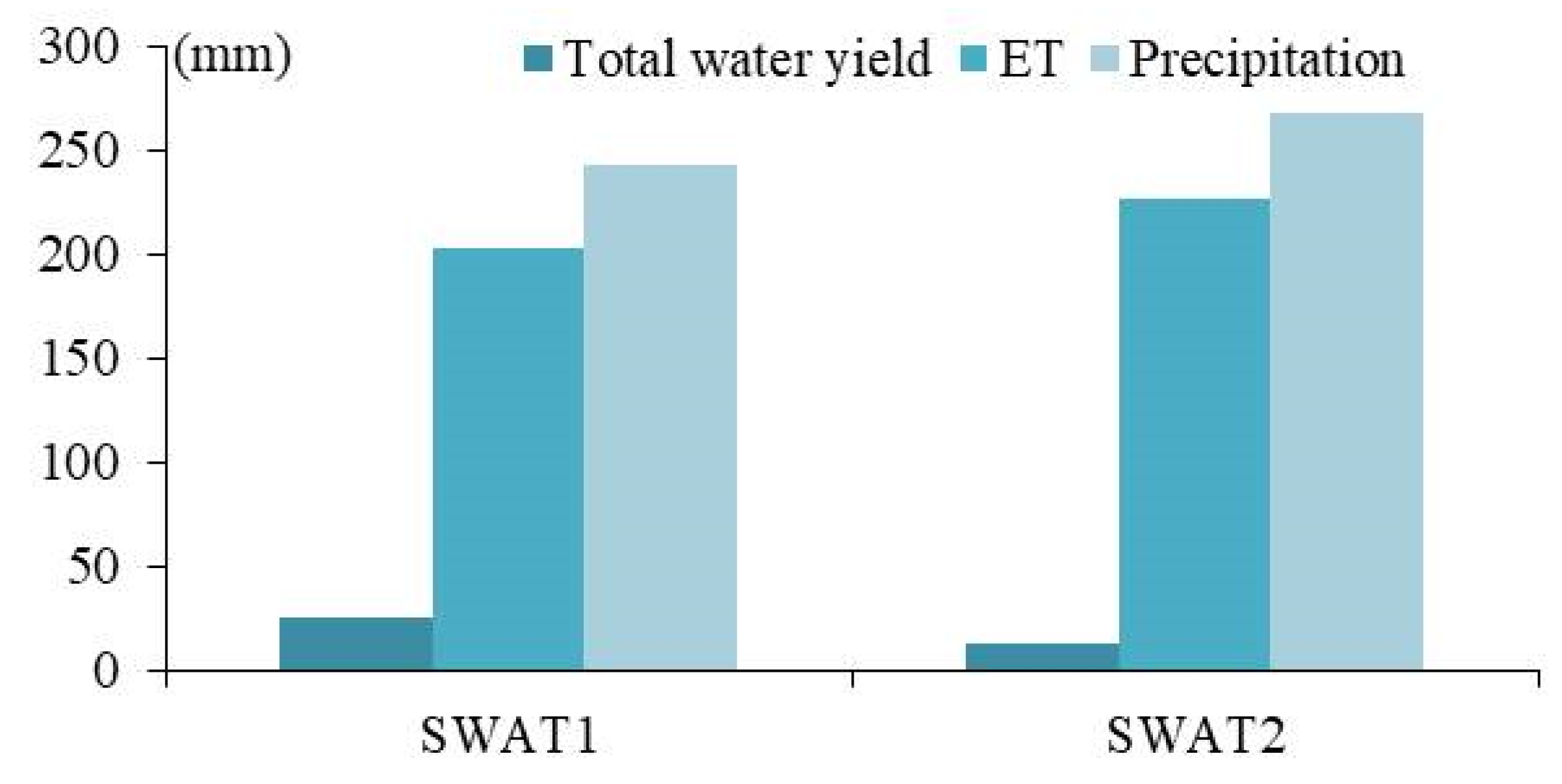
Table 4 and Figure 8 show the SWAT2M model simulation results for the streamflow in the middle reach of the Bayinhe River. The R2 and NSE values reached up to 0.78 and 0.75, respectively, and the PBIAS was within −20% to 20%. Moreover, the simulated and observed streamflows were well-matched. The performance of the SWAT2M model for simulating the monthly ET was also good (Table 4: R2 > 0.91; NSE > 0.78; PBIAS within −20% to 20%). The performance of the SWAT2M model for simulating the monthly streamflow at the outlet of the middle reach was better than that of the SWAT1 model. Figure 9 presents the monthly ET simulated by the SWAT2 model for the entire study area, whereby the simulated and observed ET were well-matched.

3.6. Water Balance

Figure 10 presents the water balance of the SWAT1 and SWAT2 models (where SWAT2 = SWAT2U + SWAT2M). It is obvious that the total water yield of the SWAT1 model was higher than that of the SWAT2 model, which resulted in a lower total simulated streamflow by the SWAT2 models. In addition, the precipitation and ET of the SWAT1 model were lower than those of the SWAT2 models. This was because different calibration data may result in different model parameter values and different water components. Compared to other research in similar study areas [7,24,25], the simulated water balance of the Bayinhe River basin by the SWAT1 and SWAT2 models was reasonable.

4. Discussion

The performance of the non-calibrated SWAT model was quite poor because the precipitation data were obtained from the only meteorological station in the watershed—in the middle reaches of the Bayinhe River, which is not representative of the rainfall across the entire upper and middle reaches. This indicates that a great effort was required to calibrate the SWAT model to obtain a better model performance. The study area of the upper and middle reaches includes variations in climate, terrain, and land use. However, as mentioned, only one hydrological station exists in the entire watershed, at the outlet of the middle reaches. Therefore, we first calibrated the SWAT model (SWAT1) using only the observed streamflow at the outlet of the middle reach. Compared to the non-calibrated SWAT model, the performance of the calibrated SWAT1 model to simulate the monthly streamflow improved obviously. The traditional calibration using the site-based streamflow grouped the hydrological processes together, which was primarily due to there being only one gauging station. Hence, this situation illustrates the need for more data with a high spatial resolution to calibrate the SWAT model for such a data scarce area.
To address this issue, the SWAT2 model was calibrated with both the site-based streamflow and satellite-based ET data. In addition, the upper and middle reaches were calibrated separately (SWAT2U and SWAT2M). The SWAT2U model simulated the water balance of the upper reach of the Bayinhe River and was calibrated using the GLEAM-based ET data, whereas the SWAT2M model simulated the water balance of the middle reach of the Bayinhe River and was calibrated using the GLEAM-based ET data and observed stream outflow from the middle reach. For the SWAT2M, the simulated stream outflow from the upper reach was used directly as the inflow to the middle reach. The performances of the SWAT2U and SWAT2M models for simulating the monthly ET were very good. The performance of the SWAT2M model for simulating the monthly streamflow at the outlet of the middle reach was better than that of the SWAT1 model. Although other similar studies [16,17,18] have used different ET data to calibrate their hydrological models, our results, which used the satellite-based ET data to improve our model’s performance, were essentially the same as these previous studies. In our research, the GLEAM-based ET data played four roles in the calibration process, whereby the data: (1) distributed the hydrological processes of the study area (compared to SWAT1); (2) reduced the uncertainty of the SWAT model in this data scarce area; (3) improved the performance of the SWAT model to simulate the streamflow and water balance; (4) improved the reliability of the model parameters.
As mentioned, the precipitation data used in the present study were obtained from the only meteorological station in the study area; thus, the spatial heterogeneity of precipitation was not considered. This may have been a factor for the discrepancy between the simulated and observed streamflow in some specific months. Hence, if the spatial heterogeneity of precipitation had been taken into account, the model uncertainties may have been reduced. Although the use of the GLEAM-based ET data to calibrate the SWAT model improved the model’s performance for simulating the streamflow, the performance was not very good. Consequently, validated satellite-based precipitation data are needed for hydrological modelling in such data scarce areas.
In this research, we assumed that the GLEAM-based ET data could provide an independent measure of ET. Although the dataset was validated for the entire area of China, the GLEAM is just a series of algorithms to calculate ET, and some deviation still exists in comparison to field observed ET. Moreover, the spatial resolution of the GLEAM-based ET data is 0.25° × 0.25°, with one data point corresponding to one or more sub-basins. The use of the GLEAM dataset was able to reduce the grouping of hydrological processes that occurred during the model calibration. However, an equifinality issue may still have occurred at the HRU scale [16]. Further study is therefore required to downscale the GLEAM-based ET data and improve the calibration results in HRUs.

5. Conclusions

In this research, three SWAT models (SWAT1, SWAT2U, and SWAT2M) were built to evaluate the advantages of using ET data derived from the GLEAM to separately calibrate the widely used SWAT model for the upper and middle reaches of a scare data area: The Bayinhe River. The results showed that:
(1) A great effort was required to calibrate the SWAT model for the Bayinhe River basin to obtain a better model performance;
(2) The performance of the SWAT model to simulate the streamflow and water balance was reliable when calibrated with streamflow only; however, this calibration method grouped the hydrological processes together and caused an equifinality issue;
(3) The combination of the streamflow and GLEAM-based ET data for the SWAT model calibration improved the model’s performance for simulating the streamflow and water balance. However, the equifinality issue remained at the HRU level.

Author Contributions

Conceptualisation, Y.J. and X.J.; Writing—original draft preparation, Y.J. and X.J.; Software—X.J. All authors have read and agreed to the published version of the manuscript.

Funding

This research was funded by the National Natural Science Foundation of China (No. 41,801,094) and grants from the Natural Science Foundation of Qinghai Province (No. 2019-ZJ-939Q).

Acknowledgments

We thank the reviewers for their constructive comments and suggestions to improve the early version of this paper.

Conflicts of Interest

The authors declare no conflict of interest.

Data Availability

The data used to support the findings of this study are included within the article.

References

  1. Rodriguez, F.; Hervé, A.; Morena, F. A distributed hydrological model for urbanized areas-Model development and application to case studies. J. Hydrol. 2008, 351, 268–287. [Google Scholar] [CrossRef]
  2. Roshan, S.; Yasuto, T.; Kaoru, T. Input data resolution analysis for distributed hydrological modeling. J. Hydrol. 2006, 319, 36–50. [Google Scholar]
  3. Jin, X.; Zhang, L.; Gu, J.; Zhao, C.; Tian, J.; He, C. Modelling the impacts of spatial heterogeneity in soil hydraulic properties on hydrological process in the upper reach of the Heihe River in the Qilian Mountains, Northwest China. Hydrol. Process. 2015, 29, 3318–3327. [Google Scholar] [CrossRef]
  4. Wang, Y.; Brubaker, K. Implementing a nonlinear groundwater module in the soil and water assessment tool (SWAT). Hydrol. Process. 2014, 28, 3388–3403. [Google Scholar] [CrossRef]
  5. Pohlert, T.; Breuer, L.; Huisman, J.A.; Frede, H.G. Assessing the model performance of an integrated hydrological and biogeochemical model for discharge and nitrate load predictions. HESS 2007, 11, 997–1011. [Google Scholar] [CrossRef] [Green Version]
  6. Noori, N.; Kalin, L. Coupling SWAT and ANN models for enhanced daily streamflow prediction. J. Hydrol. 2016, 533, 141–151. [Google Scholar] [CrossRef]
  7. Jin, X.; He, C.; Zhang, L.; Zhang, B. A Modified Groundwater Module in SWAT for Improved Streamflow Simulation in a Large, Arid Endorheic River Watershed in Northwest China. Chin. Geogr. Sci. 2018, 28, 49–62. [Google Scholar] [CrossRef] [Green Version]
  8. Hartwich, J.; Schmidt, M.; Bölscher, J.; Reinhardt-Imjela, C.; Murach, D.; Schulte, A. Hydrological modelling of changes in the water balance due to the impact of woody biomass production in the North German Plain. Environ. Earth Sci. 2016, 75, 1071. [Google Scholar] [CrossRef]
  9. Arnold, J.G.; Moriasi, D.N.; Gassman, P.W.; Abbaspour, K.C.; White, M.J.; Srinivasan, R.; Kannan, N. SWAT: Model use, calibration, and validation. Trans. ASABE 2012, 55, 1345–1352. [Google Scholar] [CrossRef]
  10. Santosh, G.; Kolladi, Y.; Surya, T. Influence of Scale on SWAT Model Calibration for Streamflow in a River Basin in the Humid Tropics. Water Resour. Manag. 2010, 24, 4567–4578. [Google Scholar]
  11. Yesuf, H.M.; Melesse, A.M.; Zeleke, G.; Alamirew, T. Streamflow prediction uncertainty analysis and verification of SWAT model in a tropical watershed. Environ. Earth Sci. 2016, 75, 806. [Google Scholar] [CrossRef]
  12. Fisher, J.B.; Tu, K.P.; Baldocchi, D.D. Global estimates of the land–atmosphere water flux based on monthly AVHRR and ISLSCP-II data, validated at 16 FLUXNET sites. Remote Sens. Environ. 2008, 112, 901–919. [Google Scholar] [CrossRef]
  13. Mu, Q.; Zhao, M.; Running, S.W. Improvements to a MODIS global terrestrial evapotranspiration algorithm. Remote Sens. Environ. 2011, 115, 1781–1800. [Google Scholar] [CrossRef]
  14. Miralles, D.G.; Holmes, T.R.H.; De Jeu, R.A.M.; Gash, J.H.; Meesters, A.G.C.A.; Dolman, A.J. Global land-surface evaporation estimated from satellite-based observations. HESS 2010, 7, 8479–8519. [Google Scholar] [CrossRef] [Green Version]
  15. Chen, Y.; Xia, J.; Liang, S.; Feng, J.; Fisher, J.B.; Li, X.; Li, X.; Liu, S.; Ma, Z.; Miyata, A.; et al. Comparison of satellite-based evapotranspiration models over terrestrial ecosystems in China. Remote Sens. Environ. 2014, 140, 279–293. [Google Scholar] [CrossRef]
  16. Immerzeel, W.W.; Droogers, P. Calibration of a distributed hydrological model based on satellite evapotranspiration. J. Hydrol. 2008, 349, 411–424. [Google Scholar] [CrossRef]
  17. Rientjes, T.H.M.; Muthuwatta, L.P.; Bos, M.J.; Bhatti, H.A. Multi-variable calibration of a semi-distributed hydrological model using streamflow data and satellite-based evapotranspiration. J. Hydrol. 2013, 505, 276–290. [Google Scholar] [CrossRef]
  18. Parajuli, P.B.; Jayakody, P.; Ouyang, Y. Evaluation of Using Remote Sensing Evapotranspiration Data in SWAT. Water Resour. Manag. 2017, 32, 985–996. [Google Scholar] [CrossRef]
  19. Yang, X.; Wang, G.; Pan, X.; Zhang, Y. Spatio-temporal variability of terrestrial evapotranspiration in China from 1980 to 2011 based on GLEAM data. Trans. Chin. Soc. Agric. Eng. 2015, 31, 132–141, (in Chinese with English Abstract). [Google Scholar]
  20. Zhang, L.; Nan, Z.; Xu, Y.; Li, S. Hydrological Impacts of Land Use Change and Climate Variability in the Headwater Region of the Heihe River Basin, Northwest China. PLoS ONE 2016, 11, 1–25. [Google Scholar] [CrossRef]
  21. Jin, X.; Jin, Y.X.; Mao, X.F. Ecological risk assessment of cities on the Tibetan Plateau based on land use/land cover changes—Case study of Delingha City. Ecol. Indic. 2019, 101, 185–191. [Google Scholar] [CrossRef]
  22. Stannard, D.I. Comparison of Penman-Monteith, Shuttleworth-Wallace, and Modified Priestley-Taylor Evapotranspiration Models for wildland vegetation in semiarid rangeland. Water Resour. 1993, 29, 1379–1392. [Google Scholar] [CrossRef]
  23. Moriasi, D.N.; Arnold, J.G.; Van Liew, M.W.; Bingner, R.L.; Harmel, R.D.; Veith, T.L. Model Evaluation Guidelines for Systematic Quantification of Accuracy in Watershed Simulations. Trans. ASABE 2007, 50, 885–900. [Google Scholar] [CrossRef]
  24. Li, Z.; Xu, Z.; Shao, Q.; Yang, J. Parameter estimation and uncertainty analysis of SWAT model in upper reaches of the Heihe River basin. Hydrol. Process. 2009, 23, 2744–2753. [Google Scholar] [CrossRef]
  25. Yang, L.; Feng, Q.; Yin, Z.; Wen, X.; Si, J.; Li, C.; Deo, R.C. Identifying separate impacts of climate and land use/cover change on hydrological processes in upper stream of Heihe River, Northwest China. Hydrol. Process. 2017, 31, 1100–1113. [Google Scholar] [CrossRef]
Figure 1. (a) Bayinhe watershed study area and (b) its location in the Qaidam basin.
Water 12 00897 g001
Figure 2. Soil and Water Assessment Tool (SWAT) model basic data. (a) Soil types; (b) land use types; (c) sub-basins.
Water 12 00897 g002
Figure 3. Soil and Water Assessment Tool (SWAT) model calibration strategy. ET: evapotranspiration; GLEAM: Global Land surface Evaporation Amsterdam Methodology.
Water 12 00897 g003
Figure 4. Non-calibrated Soil and Water Assessment Tool (SWAT) model simulated monthly streamflow at the outlet of the middle reach.
Water 12 00897 g004
Figure 5. Soil and Water Assessment Tool (SWAT)-1 model simulated monthly streamflow at the outlet of the middle reach.
Water 12 00897 g005
Figure 6. (a) Simulated evapotranspiration (ET) by the Soil and Water Assessment Tool (SWAT)-2U model; (b) observed ET from the Global Land surface Evaporation Amsterdam Methodology (GLEAM).
Water 12 00897 g006
Figure 7. Simulated streamflow out of the upper reaches.
Water 12 00897 g007
Figure 8. Soil and Water Assessment Tool (SWAT)-2M simulated monthly streamflow at the outlet of the middle reach.
Water 12 00897 g008
Figure 9. Soil and Water Assessment Tool (SWAT)-2 simulated monthly evapotranspiration (ET).
Water 12 00897 g009
Figure 10. Water balance simulated by the Soil and Water Assessment Tool (SWAT)-1 and SWAT2 models. ET: Evapotranspiration.
Water 12 00897 g010
Table 1. Variables to calculate the actual evapotranspiration (ET) in the Global Land surface Evaporation Amsterdam Methodology (GLEAM).
VariablesDatasetsDatasets Description
Solar radiationERA-interimEuropean Centre for Medium-Range Weather Forecasts (ECMWF) Interim Re-Analysis data
Air temperatureERA-interimEuropean Centre for Medium-Range Weather Forecasts (ECMWF) Interim Re-Analysis data
PrecipitationMSWEP v2.2Multi-Source Weighted-Ensemble Precipitation version 2.2
Snow water equivalentGLOBSNOW L3A v2 & NSIDC v01GLOBSNOW version 2 and the National Snow and Ice Data Center version 01
Vegetation optical thicknessLPRMLand Parameter Retrieval Model
Surface soil waterESA-CCI v4.3European Space Agency’s Climate Change Initiative version 4.3
Table 2. Sensitivity parameters of the Soil and Water Assessment Tool (SWAT) models: SWAT1, SWAT2U and SWAT2M.
SWAT1SWAT2USWAT2M
Sensitivity Parameterst-Statp-valueSensitivity Parameterst-Statp-valueSensitivity Parameterst-Statp-value
CN2−27.090.00CN2−29.160.00CN235.310.00
CH_K27.890.00SOL_BD−7.830.00SOL_BD17.820.00
SOL_BD−6.000.00SOL_K−3.450.00SLSUBBSN−15.890.00
CH_N25.010.00ESCO2.860.00SOL_K13.470.00
SOL_K−3.870.00SLSUBBSN2.310.02HRU_SLP4.030.00
SOL_AWC−2.480.01GWQMN−1.820.07ALPHA_BF−3.880.00
GW_REVAP1.960.05SMFMN1.190.23SOL_AWC2.970.00
GWQMN−1.750.08SNOCOVMN−1.170.24ESCO2.610.01
SLSUBBSN1.650.10SNO50COV−0.960.34GW_REVAP2.070.04
SMFMN1.070.19CH_N2−0.830.39GWQMN1.890.07
CN2: SCS runoff curve number; CH_K2: effective hydraulic conductivity in main-channel alluvium; SOL_BD: moist bulk-density; CH_N2: Manning’s “n” value for the main channel; SOL_K: saturated hydraulic-conductivity; SOL_AWC: available water capacity of the soil layer; GW_REVAP: a groundwater “revap” coefficient; GWQMN: threshold depth of water in the shallow aquifer required for return flow to occur; SLSUBBSN: average slope length; SMFMN: annual minimum melt-rate for snow; ESCO: a soil evaporation compensation factor; SNOCOVMN: a snow-pack temperature lag factor; SNO50COV: fraction of the snow volume in a given area that corresponds to 50% of the snow cover; HRU_SLP: average slope steepness; ALPHA_BF: baseflow alpha-factor.
Table 3. Performance of the Soil and Water Assessment Tool (SWAT)-2U model to simulate the monthly evapotranspiration (ET). NSE: Nash-Sutcliff efficiency; PBIAS: percent bias; R2: coefficient of determination.
Sub-BasinIndicators
R2NSEPBIAS
10.920.8912.5
20.920.8415.4
30.910.8610.7
40.950.957.3
50.950.90−5.7
60.940.946.4
70.950.93−1.3
80.910.8610.9
90.900.8614.2
100.920.8913.4
110.950.943.3
120.920.8916.8
Table 4. Performance of the Soil and Water Assessment Tool (SWAT)-2M model to simulate the monthly streamflow and evapotranspiration (ET). NSE: Nash-Sutcliff efficiency; PBIAS: percent bias; R2: coefficient of determination.
SWAT2M OutputsLocationIndicators
R2NSEPBIAS
Streamflowoutlet0.780.7516.5
ETSub-basin 10.920.907.4
ETSub-basin 20.920.886.2
ETSub-basin 30.910.78−10.6
ETSub-basin 40.930.9012.4
ETSub-basin 50.920.916.9

