Article

Simulating the Hydrological Processes of a Meso-Scale Watershed on the Loess Plateau, China

1
College of Soil and Water Conservation, Beijing Forestry University, Beijing 100083, China
2
Key Laboratory of Soil and Water Conservation & Desertification Combating, State Forestry and Grassland Administration, Beijing Forestry University, Beijing 100083, China
3
Jixian National Forest Ecosystem Research Network Station, CNERN, Beijing Forestry University, Beijjng 100083, China
4
Department of Sediment Research, China Institute of Water Resources and Hydropower Research, Beijing 100038, China
5
College of Environmental Science and Engineering, North China Electric Power University, Beijing 102206, China
*
Author to whom correspondence should be addressed.
Water 2020, 12(3), 878; https://doi.org/10.3390/w12030878
Submission received: 13 February 2020 / Revised: 17 March 2020 / Accepted: 17 March 2020 / Published: 20 March 2020
(This article belongs to the Section Hydrology)

Abstract

:
The Soil and Water Assessment Tool (SWAT) model is widely used to simulate watershed streamflow by integrating complex interactions between climate, geography, soil, vegetation, land use/land cover and other human activities. Although there have been many studies involving sensitivity analysis, uncertainty fitting, and performance evaluation of SWAT model all over the world, identifying dominant parameters and confirming actual hydrological processes still remain essential for studying the effect of climate and land use change on the hydrological regime in some water-limited regions. We used hydro-climate and spatial geographical data of a watershed with an area of 3919 km2, located on the Loess Plateau of China, to explore the suitable criterion to select parameters for running the model, and to elucidate the dominant ones that govern the hydrological processes for achieving the sound streamflow simulation. Our sensitivity analysis results showed that parameters not passing the sensitive check (p-value < 0.05) could play a significant role in hydrological simulation rather than only the parameters with p-value lower than 0.05, indicating that the common protocol is not appropriate for selecting parameters by sensitivity screening only. Superior performance of the rarely used parameter SOL_BD was likely caused by a combination of lateral and vertical movement of water in the loess soils due to the run-on infiltration process that occurred for meso-scale watershed monthly streamflow modeling, contrasting with traditionally held infiltration excessive overland flow dominated runoff generation mechanisms that prevail on the Loess Plateau. Overall, the hydrological processes of meso-scale watershed in the region could be well simulated by the model though underestimates of monthly streamflow could occur. Simulated water balance results indicated that the evapotranspiration in the region was the main component leaving the watershed, accounting for 88.9% of annual precipitation. Surface runoff contributed to 63.2% of the streamflow, followed by lateral flow (36.6%) and groundwater (0.2%). Our research highlights the importance for selecting more appropriate parameters for distributed hydrological models, which could help modelers to better comprehend the meso-scale watershed runoff generation mechanism of the Loess Plateau and provide policy makers robust tool for developing sustainable watershed management planning in water-limited regions.

1. Introduction

The physical process-based distributed parameters hydrological models that incorporate watershed heterogeneity and spatial distribution of climate, terrain, soil, vegetation, and land uses are widely used for watershed management planning, water resources allocation, flood protection, climate and land use change assessment, and environmental and pollution control evaluation [1,2,3,4,5,6]. However, applying hydrological models in the real world is often challenged by calibration, validation, and predictability issues [7,8,9,10]. During the calibrated process, parameter sensitivity and uncertainty analysis often become a hurdle, even though hydrological models are normally calibrated to find optimal parameters set with the optimum objective functions [11,12,13]. Unless there is a careful sensitivity and uncertainty analysis, overestimation or underestimation of hydrologic regimes can cause over-design of mitigation measures or insufficient preparation for potential situation [13,14].
The Soil and Water Assessment Tool (SWAT) model is one of the most widely used physical processes based hydrological models worldwide due to its capability to model the full spectrum of hydrological processes and its user-friendly interface [15,16,17,18]. Moreover, capability of SWAT-CUP program that comprises a semi-automated approach (SUFI-2) can help users conduct sensitivity and uncertainty analysis in a more rigorous way [10,19]. Most of the previous studies pointed out that less than ten parameters were sufficient to represent simple rainfall-runoff processes through models [20,21,22]. However, the result of acceptable simulation of streamflow in a watershed does not signify a correct performance of runoff generation processes [23]. Because of the large number of parameters in the comprehensive watershed model, parameterization and calibration of the model become complicated [10]. All parameters governing the hydrologic processes can be used for calibrated SWAT model, and many parameters have the impact on multiple processes [10]. However, correct parameterization cannot only make model calibration be faster, be more accurate, and have lower prediction uncertainty [10], but also describe the complete hydrological cycle [6,24].
Some of the frequently used calibrated parameters that have been considered as the most sensitive parameters in controlling hydrological processes are SCS runoff curve number (CN2), soil evaporation compensation factor (ESCO), available water capacity (SOL_AWC), groundwater delay (GW_DELAY), snowfall temperature (SFTMP), baseflow alpha factor (ALPHA_BF), and surface runoff lag time (SURLAG) [6,14,15,17,23,25,26,27,28]. Most of the previous studies suggested that CN2 is the most sensitive parameter for simulating streamflow on the Loess Plateau as the infiltration excessive runoff generation mechanisms prevail for small watersheds in the region [3,20,28,29]. Nevertheless, recent studies have noted that rarely used parameters, such as moist bulk density (SOL_BD), may also be more sensitive in streamflow simulation, not only for the small watershed in humid region [30], but also for large-scale watersheds on the Loess Plateau. For example, Gong et al. (2017) identified that SOL_BD was the most sensitive parameter rather than CN2 for runoff simulation in Yanhe watershed (7725 km2) [31]. Such a finding was attributed to the higher permeability of loess soil in the Loess Plateau by ecological restoration, the lower rainfall intensity since the 1990s, and the deep-seated tunnel systems that may reach the channels [32,33,34]. However, it still remains unclear if and in what way such rarely used parameters should be considered for meso-scale watersheds in the region.
Although there have been many studies involving sensitivity analysis, uncertainty fitting and performance evaluation of SWAT model all over the world [2,11,14,16,18,35], identifying dominant parameters, reducing the magnitude of uncertainties for streamflow simulation and confirming actual hydrological processes still remain essential for some distinct regions. Uncertainties in hydrological modeling come from input data, model structure, and parameters [2,21]. However, there are many key parameters in a watershed that describe the bio-geophysical characteristics and hydrological processes of the watershed, among which some parameters are hard to measure directly and can be gained only by empirical estimation and literature references, resulting in the increased uncertainties of the modeling system [11,17,21,36]. Several studies showed that using more informative data, modified model structures, or more parameter sets could reduce uncertainties [2,37,38]. In addition, the SUFI-2 method is capable of assessing the uncertainties from all sources for the SWAT model [21]. Moreover, the parameters cannot be identified easily due to the phenomenon of equifinality [13]. Therefore, a scientific understanding of model uncertainties effect on the model performance and capacity of model to capture hydrologic processes can help users apply the model in a more rigorous way.
Most notably, the implementation of a large-scale land-conversion program, e.g., converting from agriculturally used slope land into forest or/and grassland in the Loess Plateau region of China has raised wide concerns over the water yield decrease, water carrying capacity of forest coverage, and balance between afforestation and food production [39,40]. However, changes in hydrological processes and watershed balance components associated with land use and land cover change are integrated elements for assessing the ecosystem services and healthy status at watershed scale [20,29,41,42]. Clearly, it is the physical-processes-based distributed-parameter hydrological models that can achieve such objectives. However, the models require a considerable number of parameters for their performance evaluation, including parameterization and calibration. Here, we used long-term hydro-climate data combined with land use/land cover change data interpreted from remote-sensing images, soil distribution, and landform data of Xinshui watershed located on the Loess Plateau, one of the main tributaries in the middle reach of the Yellow River, China, to investigate the applicability of SWAT model, hydrological processes, and water balance dynamics. Our specific aims are to (1) explore the suitable criterion to select parameters for running the model by challenging general protocol of sensitivity screening; (2) elucidate the dominant parameters that govern the hydrological processes for achieving the sound streamflow simulation at meso-scale watersheds that are traditionally assumed infiltration excessive overland runoff generation mechanisms prevail; and (3) quantify the long-term water balances for developing sustainable watershed management plan in the region.

2. Materials and Methods
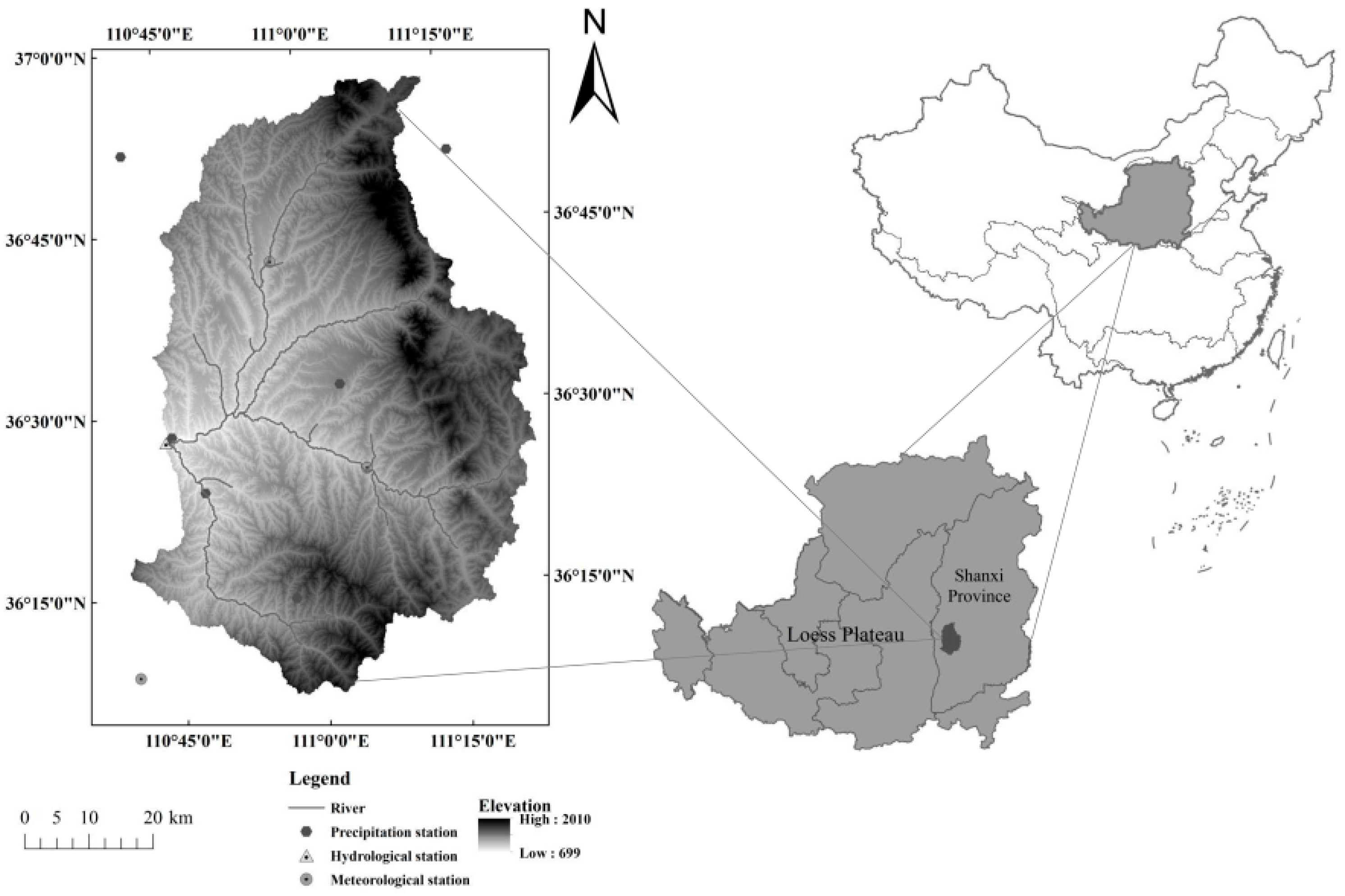
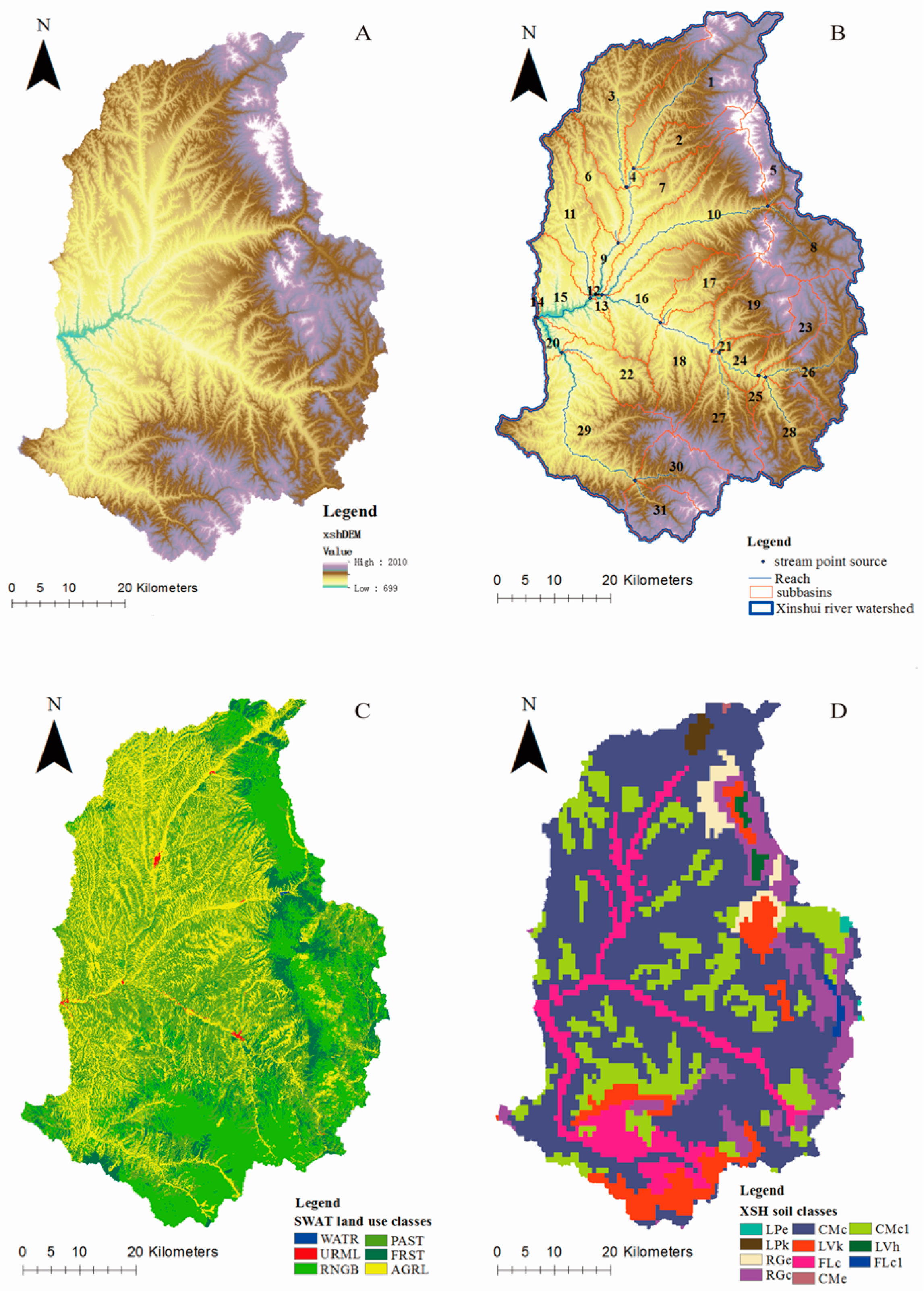
2.1. Study Area

The Xinshui watershed lies in the southeastern part of the Loess Plateau, Shanxi Province, Northern China. The river originated from the Lvliang Mountains and is the secondary contributor to the Yellow River. The drainage area is approximately 3919 km2 (36°36′–36°57′N, 110°30′–111°27′E) (Figure 1). Temperate continental monsoon climate dominates the region. The annual average temperature ranges from 7.9 to 10.7 ℃, and rainfall is from 289 to 778 mm, during the past 60 years. The watershed terrain is dominated by mountain ranges, hills, and valleys. The watershed elevation varies from 699 to 2010 m (Figure 1). Fifty-five percent of the watershed is covered by Calcaric Cambisols, while other soil types include Calcic Luvisols, Calcaric Fluvisols, Eutric Leptosols, Rendzic Leptosols, Eutric Regosols, Calcaric Regosols, Haplic Luvisols, and Eutric Cambisols. The texture of these soils is sandy loam soil composed by the sand and silt, with minor clay. Land-use types and percentage of each land use within the watershed are 7.48% forestland, 26.20% shrubland, 37.81% grassland, 28.31% cropland, 0.18% residential areas and built-in land, and 0.02% water body. Grassland is the most dominant land-use type. The major agricultural crops are corn, soybean, wheat, potato, and sorghum. Major forest types are Quercus liaotungensis, Betula platyphylla Suk, Populus davidiana, Pinus tabulaeformis, Platycladus orientalis, and Robinia pseudoacacia Linn.

2.2. SWAT Structure

The SWAT model is a typical semi-distributed, process-based hydrologic model [43]. It has a strong physical foundation for runoff generation and can simulate water, sediments, and nutrients from individual sub-watersheds to its outlet in a basin [43]. During the construction of the SWAT project, the watershed separates to sub-basins by watershed delineation according to DEM data, and some Hydrological Response Units (HRUs) constitute one sub-basin. The HRU is unique and consists of one slope type, one soil type, and one land-use type [43]. The water-balance equation in SWAT is as follows:
S W t = S W 0 + i = 1 t ( P d a y R s u r f E T a w s e e p R g w )
where SWt and SW0 means the final and the initial soil water content, respectively; t means the time; Pday means precipitation; Rsurf means surface runoff; ETa means the actual evapotranspiration; wseep means the water entering the vadose zone; and Rgw means the return flow.
The hydrologic cycle is climate driven [10]. The primary elements of hydrologic processes of the SWAT model are evapotranspiration, infiltration, surface runoff, return flow, lateral flow, tile drainage, water stored in the soil profile, and transmission losses [10]. The plant-growth model within the SWAT model simulates all land-cover types and is capable of distinguishing annual and perennial vegetation, in order to evaluate biomass production and transpiration [10]. Curve number method is used for predicting surface runoff [10]. Channel routing is estimated by the Muskingum method [15].
The water-balance equation for a closed drainage basin is as follows [44]:
P = ET + R + Δ S
where P = precipitation (mm); ET = evapotranspiration (mm); R = water yield (mm); ∆S = Sj − Si = soil water storage change (mm); and ∆S= 0 at longer time intervals.
In this study, 1986–1999 climatic inputs, land-use data and soil data were used to rerun the calibrated model and combined with the water-balance equation, to identify the proportions of hydrological elements in the watershed.

2.3. Data Preparation and Model Construction

The basic data required to build the SWAT model are weather data, digital elevation model (DEM) data, soil data, and land-use data [43]. The soil database and weather generator database need to be site-specific, and these data are introduced in detail below.
The DEM (Figure 2A) data with a resolution of 30 m × 30 m were downloaded from Geospatial Data Cloud site of Chinese Academy of Sciences, which was used for watershed delineation, stream creation, slope gradient, and channel slope extraction (Figure 2B).
Land-use data in 1995 were obtained from Landsat5 TM satellite remote sensing image product and processed by ENVI software (The Environment for Visualizing Images, version 5.1, Exelis Visual Information Solutions, Herndon, VA USA), at a 30 m resolution. The accuracy of the classification was then verified, yielding 1995 Kappa coefficient of 0.771 [20]. Six categories were obtained by classifying land use: urban and built-up areas, water, forest, shrub, grassland, and cropland. These six categories were transformed into URML, WATR, FRST, RNGB, PAST, AGRL, respectively, in the SWAT project (Figure 2C). Each land use had different surface vegetation types which influence runoff, evapotranspiration, and groundwater in the watershed. Before the large-scale Land Conversion Program (e.g., Grain for Green) was implemented since 1999, there had been no very significant land-use and land-cover changes in the region from 1986 to 1999, due to the progressive implementation of Three North Shelterbelt Programs started in 1978 [45]; therefore, we used this land-use data for our simulation, both for calibration and validation periods.
The soil database (1 km resolution) was obtained from the Harmonized World Soil Database (HWSD) and was cut out by the grid map of the study area [2]. Since SWAT used FAO soil grading, we did not convert the soil particle size content. We used SPAW software (Washington State University, WA, USA) to calculate available water content, saturated hydraulic conductivity, and matric bulk density for different layers of each soil type [43]. Other values in the soil database were calculated by the equations from SWAT documentation. Therefore, we reclassified our study soil types into 11 subtypes (Figure 2D).
Climatic inputs for running SWAT included daily wind speed, solar radiation, relative humidity, maximum and minimum temperature, and precipitation. Because the ArcSWAT tool (USDA-ARS Grass-land, Soil and Water Research Laboratory and the Texas AgriLife Blackland Research Center in Temple, Texas, USA) allows users to load weather station locations into the current project and assign weather data to the sub-watersheds, these data were then transformed into appropriate text format of SWAT project. We used three meteorological stations (from Xi County, Ji County, and Houma City) and six rainfall stations (from Daning, Majiayao, Sanduo, Xiali, Guxian, and Jiaokou) in the project (Figure 1). Sub-watershed climate data were furnished by the station nearest to the centroid of the sub-basin that achieves the point weather data to watershed weather data. The Penman–Monteith method was applied to calculate potential evapotranspiration.
Our SWAT model generated 31 sub-basins and 845 HRUs, by setting a threshold of 2%, 5%, and 10% for land use/land cover, slope, and soil types, respectively. The aim of setting thresholds is to ignore unneeded large number of HRUs [43].

2.4. SUFI-2 Method Description

2.4.1. Sensitivity Analysis

The first step of model calibration and validation is sensitivity analysis. Its primary objective is to identify parameters that have a great influence on model outputs (e.g., streamflow). We selected the global sensitivity analysis method to determine sensitive parameters, using the SUFI-2 method of SWAT-CUP [19]. Global sensitivity analysis distinguishes the sensitive rank of whole considered parameters related to streamflow by Latin hypercube regression analysis [19].
The t-stat and p-value, two statistical measurements, could assess the sensitive rank of each parameter. The t-stat represents a range of sensitivity, while the p-value identifies the significance of sensitivity. Higher absolute value of t-stat and lower value of p-value (<0.05) indicate that a parameter is sensitive [17].
Twenty-four input parameters for running SWAT model were selected for sensitivity analysis according to the literature review from watersheds with similar characteristic to Xinshui watershed of the Loess Plateau (Table 1) [10,20,28,30,35].

2.4.2. Uncertainty Analysis

The values of P-factor and R-factor in SUFI-2 algorithm of SWAT-CUP, were applied to assess the SWAT model simulation uncertainties [19]. P-factor is the percentage of measured data enveloped by model simulation results, 95PPU. R-factor is 95PPU envelope thickness [19]. All the uncertainty factors (including driving variables, parameters, observed data, conceptual model, etc.) in the whole process of simulation can be accounted by parameter uncertainty [15]. Therefore, for streamflow, if the P-factor is higher than 70% and the R-factor is lower than 1, that means the simulation results are acceptable [19].

2.4.3. Calibration and Validation

Our SWAT monthly streamflow was calibrated in comparison with the monthly observed streamflow at Daning Hydrological Station of Xinshui watershed. The model was implemented for 17 years, from 1983 to 1999, by applying the first 3 years for warm-up period, allowing the hydrologic cycle to be fully represented in the model. Calibration data were from 1986 to 1992, whereas validation data were from 1993 to 1999. Land-use data in 1995 were applied to ensure high accuracy of land use during the whole calibrated process [46].

2.4.4. Model Performance Evaluation

We also used the NS (Nash–Sutcliffe coefficient) [47], R2 (coefficient of determination), PBIAS (percent bias), and RSR (standardize the RMSE using observation standard deviation) to determine the model performance [19].
N S = 1 j ( Q m Q s ) j 2 j ( Q m , j Q ¯ m ) 2
R 2 = [ j ( Q m , j Q ¯ m ) ( Q s , j Q ¯ s ) ] 2 j ( Q m , j Q ¯ m ) 2 j ( Q s , j Q ¯ s ) 2
P B I A S = 100 × j = 1 n ( Q m Q s ) j j = 1 n Q m , s
R S R = j = 1 n ( Q m Q s ) j 2 j = 1 n ( Q m , j Q ¯ m ) 2
where Q is streamflow; m is observed data; s is simulated data; the bar is represented for average; and j is the jth measured or simulated data.
The performance evaluation criteria (NS, R2 ≥ 0.5, PBIAS < ±25% and RSR < 0.7) means satisfactory model calibration [48].

3. Results

3.1. Sensitivity Analysis

Twenty-four hydrological parameters were tested for sensitivity analysis via the SUFI-2 method for streamflow simulation in the Xinshui River Watershed. The absolute value of t-stat ranged from 0.05 to 14.26, and the p-value ranged from 0 to 0.96 (Table 2). According to the parameter sensitivity evaluation criterion, 11 parameters passing the sensitivity check (p-value < 0.05) were SOL_BD, RCHRG_DP, GWQMN, ESCO, CN2, SLSUBBSN, OV_N, GW_DELAY, ALPHA_BNK, CH_N2, and SOL_K. Hydrologically, the SOL_BD parameter controls the horizontal and vertical movement of soil water; the RCHRG_DP and GWQMN parameters regulate the occurrence of groundwater; the ESCO parameter controls the contribution of soil water to evaporation; the CN2, SLSUBBSN, and OV_N parameters control the formation of surface runoff; the GW_DELAY and ALPHA_BNK parameters regulate the retention time of groundwater or baseflow. The CH_N2 parameter plays an important role in regard to channel flow; the SOL_K parameter controls the movement of soil water [19].

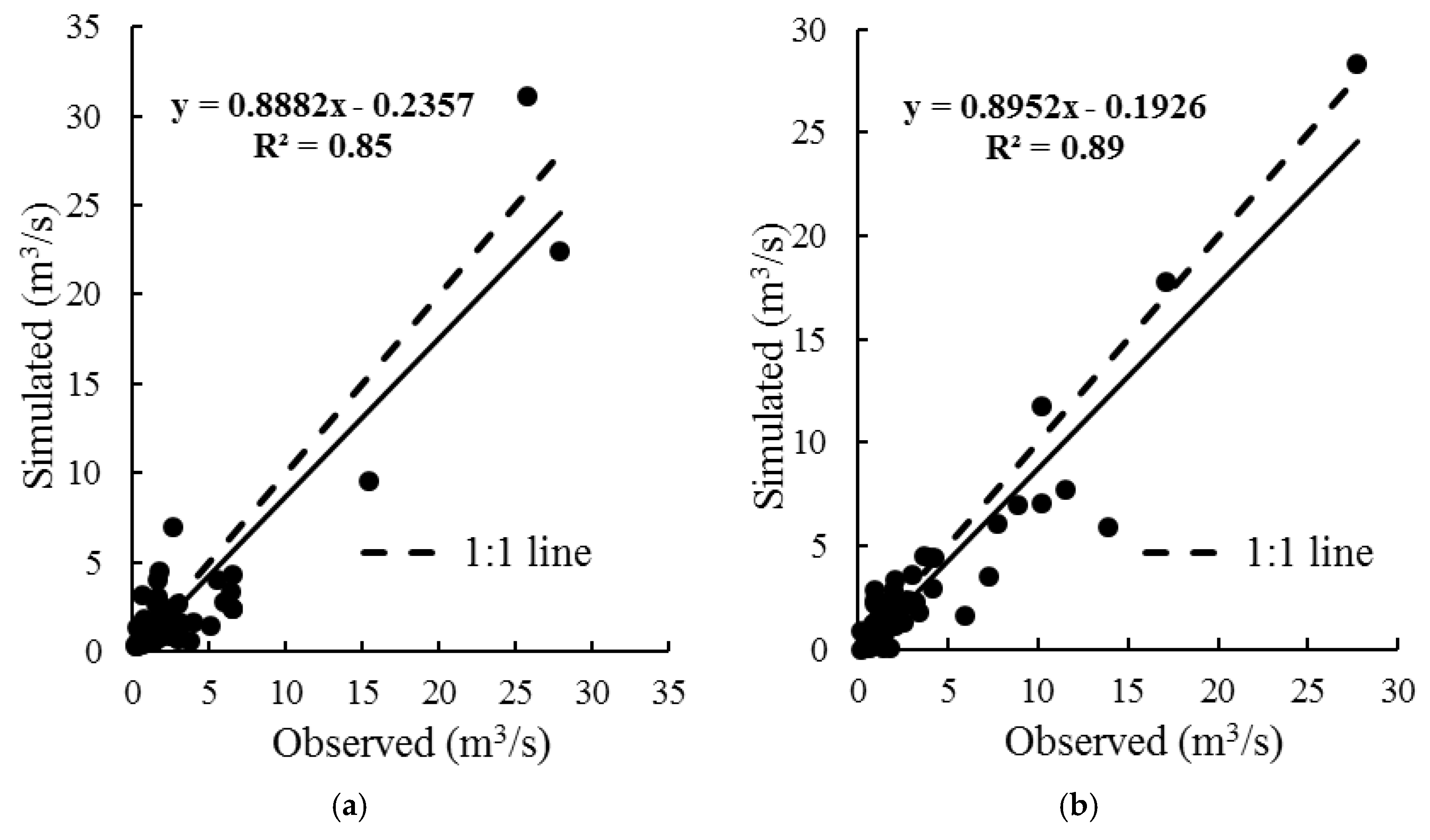
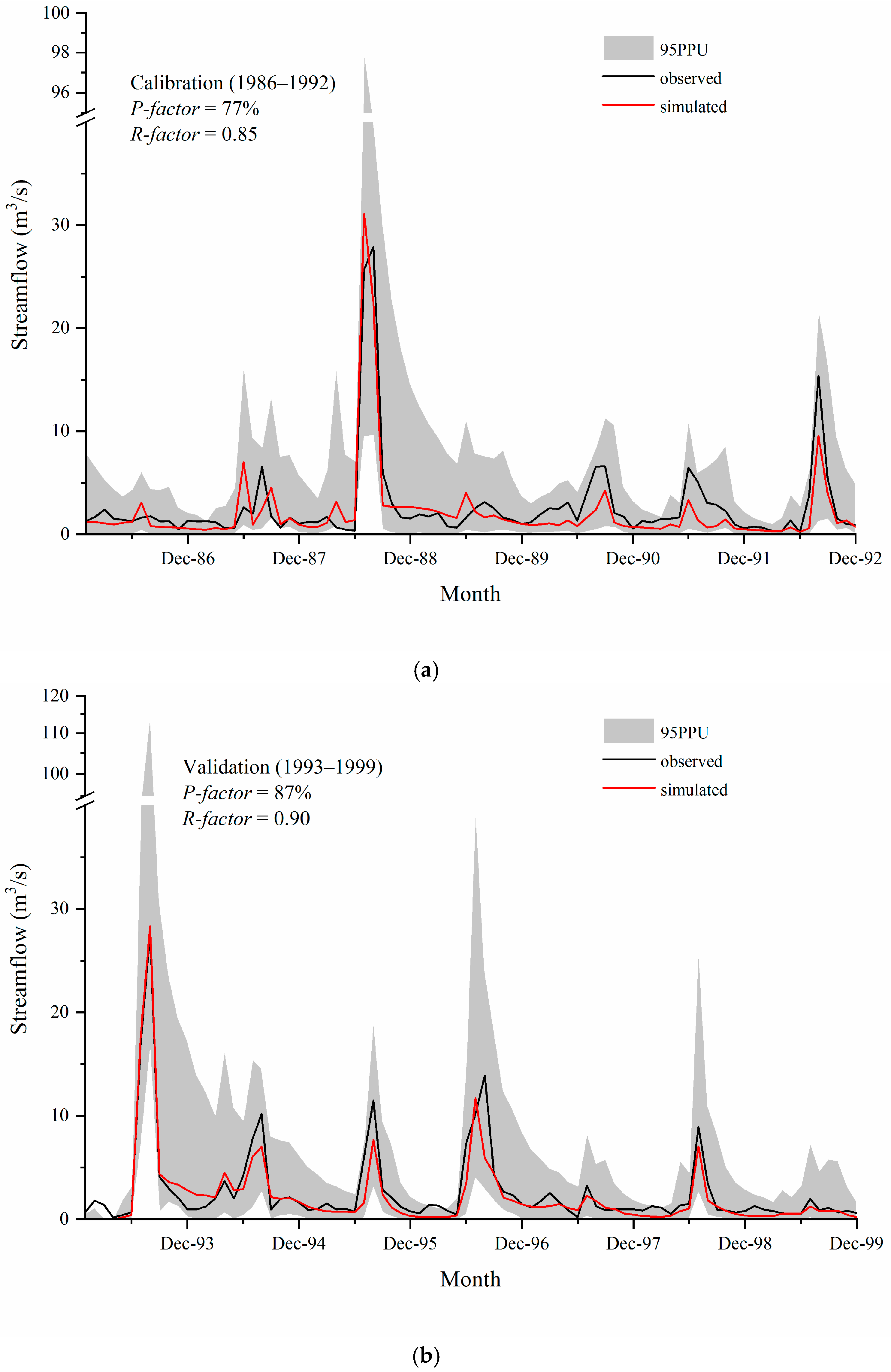
3.2. Model Calibration and Validation

Model calibration was first conducted by using the 11 parameters passing the sensitivity check (Table 2). However, model performance criteria R2, NS, PBIAS, and RSR were 0.7, 0.66, 32.3% and 0.58, respectively, indicating the simulation was unsatisfactory and erroneous. The SWAT model could satisfactorily simulate the monthly streamflow for the watershed, until the first nineteen parameters were all used for calibration (Table 3). Model performance indictors NS, RSR, and PBIAS were 0.83, 0.41, and 20% for the calibration period and 0.88, 0.35, and 17.6% for the validation period, respectively (Table 4), achieving the satisfactory level. The linear regression coefficients in calibration and validation less than 1 indicated that monthly streamflow was likely underestimated in the Xinshui River Watershed (Figure 3).

3.3. Uncertainty Analysis
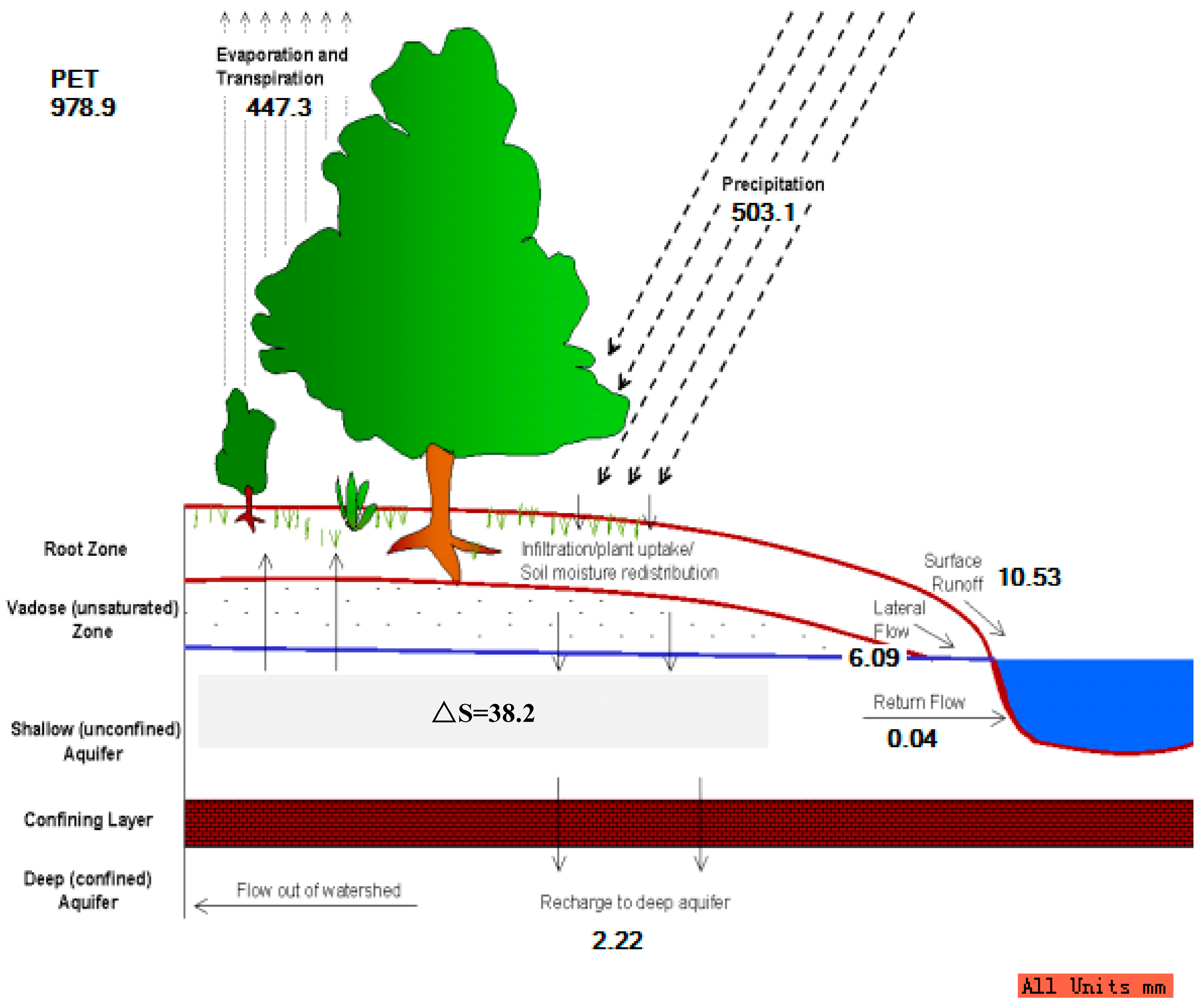
The SUFI-2 method could capture the monthly streamflow regime during the whole calibration period. First, most of the observed monthly streamflow data were within the 95PPU bracket (77% in calibration period, 87% in validation period). Second, the R-factor equaled 0.85 and 0.9, respectively, for calibration and validation periods. The simulated annual averaged streamflow during the calibration period was 2.14 m3/s, which was 20% lower than the observed data (2.68 m3/s). Similarly, the observed and simulated annual averaged streamflow during the validation period were 2.69 and 2.21 m3/s, respectively, with −17.6% simulation errors. Both results showed that some streamflow were underestimated, especially in the winter and during the flood periods in summer in 1990, 1991, and 1992 (Figure 4). However, they remained within the boundaries of 95PPU of simulated streamflow, indicating that the uncertainty of the SWAT model was within the allowable range.

3.4. Water Balances

For a watershed, precipitation, evapotranspiration, surface runoff, lateral flow, and groundwater are the most important water balance components. The long-term mean annual water balance components of the Xinshui River Watershed during 1986 to 1999 are shown in Figure 5. The distribution proportion of precipitation for water balance components was obtained by SWAT-Check tool (USDA-ARS Grass-land, Soil and Water Research Laboratory and the Texas AgriLife Blackland Research Center in Temple, Texas, USA). The incoming precipitation flux was balanced by evaporation of soils and plants (88.9%), followed by water yield (3.8%) and other components stored in soils and/or lost from channel by transmission (7.3%) (Table 5).
Similarly, the seasonal water balance from 1986 to 1999 is shown in Figure 6. The results also indicated that the amount of precipitation was lost mainly by evapotranspiration and surface runoff. Due to the dominated infiltration excessive overland runoff generation mechanism in the region, surface runoff contributed 63.2% to the total streamflow, followed by lateral flow (36.6%) and groundwater (0.2%). The baseflow, which is constituted by lateral and groundwater flow together, contributed to 36.8% of the total streamflow (Figure 6). The seasonal trend in potential evapotranspiration (PET) showed an increase trend from January to June, and then a decrease trend from July to December (Figure 6). The trend of seasonal precipitation (P), evapotranspiration (ET), water yield (WYLD), and surface runoff (SURQ) showed similar patterns during the simulation period.

4. Discussion

Sensitivity analysis usually provides a parameter selection scheme for running a physical-processes-based distributed-parameter hydrological model. All the sensitive parameters with higher absolute value of t-state and lower p-value than 0.05 are used for calibrating the SWAT model, while other parameters are treated as insensitive and not used [10,17]. However, the model performance could achieve the satisfactory level until 19 parameters calibrated (Table 3 and Table 4). This result is consistent with previous studies indicating that the good results in prediction would be achieved based on a large number of parameter sets rather than one “best” parameter set [37,49,50]. Clearly, our study suggested that the insensitive parameters could also play a role in hydrological simulation according to other model-performance evaluation criteria (R2, NS, PBIAS, P-factor, and R-factor).
In our study, the sensitivity rank of CN2 was lower than SOL_BD, RCHRG_DP, GWQMN and ESCO, suggesting that more complex hydrological processes may occur in the watershed. As the most sensitive parameter among all 19 parameters for calibrating SWAT model in the Loess Plateau, SOL_BD could significantly improve the performance of the model for simulating monthly streamflow. The performance evaluation criteria R2, NS, and RSR, without considering SOL_BD, were 0.75, 0.72, and 0.53 for calibration and 0.82, 0.81, and 0.43 for validation, accordingly. When this parameter was involved, R2, NS, and RSR were improved to 0.85, 0.83, and 0.41 for calibration and 0.89, 0.88, and 0.34 for validation, respectively (Table 4). Our sensitivity analysis results showed that SOL_BD was the most sensitive parameter, a finding that differs from the previous conclusion that CN2 is the most sensitive parameter for streamflow simulation supported by the long hold infiltration excessive overland flow runoff generation mechanism in the Loess region [3,20,28,51]. Superior performance of SOL_BD was likely caused by a combination of lateral and vertical movement of water in the loess soils, as it was also observed in the Yanhe River Basin of the Loess Plateau [31]. Hortonian overland flow (run-on infiltration process) is the main infiltration mechanism at the hillslope scale, resulting from high rainfall intensity but low duration [8]. As the Hortonian flow moves to the river channel, the movement of water via the Dunne flow (saturation excess) determines the hydrological cycle at the watershed scale [33]. Furthermore, the main soil type in the Xinshui River Watershed is Calcaric Cambisols, so low-intensity rainfall would infiltrate the soil [33]. Parameter SOL_BD is closely related with soil infiltration in that the initial infiltration capacity of soil decreases against the increase in bulk density, and the attenuation rate of infiltration capacity increase with the increase of bulk density [51,52]. These results indicated that the lateral and vertical redistribution movement of water in the soil layers into the watershed outlet had a significant effect on hydrological processes, such as later flow, groundwater, and evapotranspiration. Our study suggested that, in addition to the frequently used parameters, the rarely used parameter SOL_BD should be used for model calibration, to improve the model performance and help modelers understand the main hydrological process in the meso-scale watershed of the Loess Plateau and other similar regions in the world.
Understanding uncertainty can improve on the deeper comprehending of both hydrologic cycle and model predictions [37]. The larger the P-factor value, the greater the contribution of parameter uncertainty to the uncertainty of the simulation [2]. The lower P-factor means that input or structure may dominate model simulation uncertainty [2,38]. Our uncertainty analysis results during the validation period (P-factor = 87%, R-factor = 0.9) were better than those during the calibration period (P-factor = 77%, R-factor = 0.85), implying that parameter uncertainty contributed the most. These results suggested that using appropriate parameters makes it possible to represent model simulation uncertainty and reduce input and/or structure uncertainty. In addition, there were some underestimations of peak flows in summer, particularly during the calibration period. Monthly streamflow in this temperate monsoon climate region is usually contributed to by several thunderstorms characterized with quick response. However, simulated monthly streamflow could be tamped down by the time step of 30 days, leading to the underestimation for summer peak flows [8,33,53]. Moreover, a simplified approach in the SWAT model is employed to reckon soil temperature and confirm the frozen and thawed state of soils, and both also increase a small part of simulation uncertainty [2,40]. Uncertainties of the SWAT model were within acceptable limits, meaning that all source uncertainties were captured by parameter uncertainty in our study [15,17,21,23,54]. However, this does not neglect the significance of the spatiotemporal variability of precipitation [38,53] and model structures [2,55,56] during the whole calibration processes.
The hydrological processes of the Xinshui River Watershed were satisfactorily simulated by SWAT model in our study. The average simulated ET from 1986 to 1999 was 447.3 mm (Figure 5), and the average measurement ET (which equals to averaged P minus averaged streamflow) was 457.8 mm. Compared with measured ET, the relative error of simulated ET was only −2.3%. Our simulated results showed that the 88.9% of P returned to atmosphere through ET, and a similar result was found in Yanhe River Basin [57]. Only 3.8% of P was in form of streamflow through the watershed outlet, and the rest of P was stored in soils and/or lost from channel by transmission (7.3%). The Xinshui River Watershed, located in the Loess Plateau, under temperate continental monsoon climate, which is known to have over 80% of P, appears from May to October, and the result is consistent with [8]. SURQ and WYLD had a similar trend with P in seasonal scale because the dominated hydrologic processes were overland flow and water yield generated from thunder storms [8]. However, LATQ showed a smoother upward trend due to lateral redistribution movement of water [33]. The mean annual P (503.1 mm) was equal to the sum of ET (447.3 mm), R (18.98 mm) and (38.2 mm) was 504.17 mm, the absolute error of water balance was −1.38 mm, and the relative error was 0.3%. The reason for simulated water balance error may be the poor simulation of snowmelt process of the SWAT model [56]. Although the relative error of watershed water balance from 1986 to 1999 ranged from −2.26% to 2.17% (lower than 5%) (Table 5), the hydrologic processes simulated by SWAT model can used for further analysis. In addition, the simulated total annual water yield for 1986–1999 was 18.98 mm, which is constituted by surface runoff (63.2%) and baseflow (36.8%). The result is in accordance with Kang et al.’s (2019) finding that the average annual baseflow index in Xinshui River Watershed is 0.368 [58]. Hence, knowing the watershed hydrologic processes is helpful for mangers to make decisions on the water resources’ utilization.

5. Conclusions

In this study, the values of performance evaluation criteria (R2, NS, PBIAS, RSR, P-factor, and R-factor) during the calibration period were 0.85, 0.83, 0.41, 20.0, 77% and 0.85, while during validation period, those values were 0.89, 0.88, 0.34, 17.6, 87% and 0.9, showing that streamflow and actual hydrological processes of the Xinshui River Watershed (~4000 km2) could be modeled by using SWAT with the SUFI-2 method. However, unlike most published works, we found that more parameters used could significantly improve the model performance and sensitivity analysis may not be applicable universally for determining parameter sets. We also concluded that the inclusion of SOL_BD, the most sensitive parameter controlling the horizontal and vertical movement of soil water, could improve the model performance greatly, challenging the long-held ideas that the CN curve number is the most sensitive parameter relevant to infiltration excessive overland flow generation mechanisms in the region. It was anticipated that model uncertainty could be captured by parameters uncertainty. In addition, the watershed water-balance results suggested that most of the precipitation was evaporated into the atmosphere; therefore, only a small percentage of precipitation formed streamflow. Surface runoff is the primary component of the streamflow within the study area; the significance of baseflow in hydrological processes cannot be neglected. The calibrated SWAT model in Xinshui River Watershed can be used to explore the effect of climate and land-use-change scenarios on hydrologic cycle.

Author Contributions

Conceptualization, M.L. and Z.Z.; methodology, M.L.; software, M.L.; validation, M.L. and Z.Z.; formal analysis, M.L.; data curation, M.L.; writing, M.L., Z.Z, S.W. and Y.Y. All authors have read and agreed to the published version of the manuscript.

Funding

This research was funded by the National Science and Technology Support Project (grant number 2015BAD07B030303), and the Beijing Municipal Education Commission for their financial support through Innovative Transdisciplinary Program of Ecological Restoration Engineering.

Acknowledgments

We thank the editors and the anonymous reviewers for their constructive comments and suggestions to improve our original version of the manuscript.

Conflicts of Interest

The authors declare no conflict of interest.

References

  1. Zuo, D.; Xu, Z.; Yao, W.; Jin, S.; Xiao, P.; Ran, D. Assessing the effects of changes in land use and climate on runoff and sediment yields from a watershed in the Loess Plateau of China. Sci. Total Environ. 2016, 544, 238–250. [Google Scholar] [CrossRef] [PubMed]
  2. Zhang, X.; Xu, Y.; Fu, G. Uncertainties in SWAT extreme flow simulation under climate change. J. Hydrol. 2014, 515, 205–222. [Google Scholar] [CrossRef]
  3. Zhao, A.; Zhu, X.; Liu, X.; Pan, Y.; Zuo, D. Impacts of land use change and climate variability on green and blue water resources in the Weihe River Basin of northwest China. Catena 2015, 137, 318–327. [Google Scholar] [CrossRef]
  4. Malagó, A.; Bouraoui, F.; Vigiak, O.; Grizzetti, B.; Pastori, M. Modelling water and nutrient fluxes in the Danube River Basin with SWAT. Sci. Total Environ. 2017, 603–604, 196–218. [Google Scholar] [CrossRef]
  5. Liu, R.; Wang, Q.; Xu, F.; Men, C.; Guo, L. Impacts of manure application on SWAT model outputs in the Xiangxi River watershed. J. Hydrol. 2017, 555, 479–488. [Google Scholar] [CrossRef]
  6. Jung, C.G.; Kim, S.J. Assessment of the water cycle impact by the Budyko curve on watershed hydrology using SWAT and CO2concentrations derived from Terra MODIS GPP. Ecol. Eng. 2018, 118, 179–190. [Google Scholar] [CrossRef]
  7. Zhao, Q.; Ye, B.; Ding, Y.; Zhang, S.; Yi, S.; Wang, J.; Shangguan, D.; Zhao, C.; Han, H. Coupling a glacier melt model to the Variable Infiltration Capacity (VIC) model for hydrological modeling in north-western China. Environ. Earth Sci. 2013, 68, 87–101. [Google Scholar] [CrossRef]
  8. Zhang, Z.; Wang, S.; Sun, G.; McNulty, S.G.; Zhang, H.; Li, J.; Zhang, M.; Klaghofer, E.; Strauss, P. Evaluation of the MIKE SHE model for application in the Loess Plateau, China. J. Am. Water Resour. Assoc. 2008, 44, 1108–1120. [Google Scholar] [CrossRef]
  9. Qin, N.; Wang, J.; Chen, X.; Yang, G.; Liang, H. Impacts of climate change on regional hydrological regimes of the Wujiang River watershed in the Karst area, Southwest China. Geoenvironmental Disasters 2015, 2, 1–18. [Google Scholar] [CrossRef] [Green Version]
  10. Arnold, J.G.; Moriasi, D.N.; Gassman, P.W.; Abbaspour, K.C.; White, M.J.; Srinivasan, R.; Santhi, C.; Harmel, R.D.; Van Griensven, A.; VanLiew, M.W.; et al. Swat: Model Use, Calibration, and Validation. Asabe 2012, 55, 1491–1508. [Google Scholar] [CrossRef]
  11. Her, Y.; Yoo, S.H.; Cho, J.; Hwang, S.; Jeong, J.; Seong, C. Uncertainty in hydrological analysis of climate change: Multi-parameter vs. multi-GCM ensemble predictions. Sci. Rep. 2019, 9, 1–22. [Google Scholar] [CrossRef] [PubMed] [Green Version]
  12. Kouchi, D.H.; Esmaili, K.; Faridhosseini, A.; Sanaeinejad, S.H.; Khalili, D.; Abbaspour, K.C. Sensitivity of calibrated parameters and water resource estimates on different objective functions and optimization algorithms. Water 2017, 9, 384. [Google Scholar] [CrossRef] [Green Version]
  13. Shen, Z.Y.; Chen, L.; Chen, T. Analysis of parameter uncertainty in hydrological and sediment modeling using GLUE method: A case study of SWAT model applied to Three Gorges Reservoir Region, China. Hydrol. Earth Syst. Sci. 2012, 16, 121–132. [Google Scholar] [CrossRef] [Green Version]
  14. Setegn, S.G.; Srinivasan, R.; Melesse, A.M.; Dargahi, B. SWAT model application and prediction uncertainty analysis in the Lake Tana Basin, Ethiopia. Hydrol. Process. 2010, 24, 357–367. [Google Scholar] [CrossRef]
  15. Zhou, J.; Liu, Y.; Guo, H.; He, D. Combining the SWAT model with sequential uncertainty fitting algorithm for stream flow prediction and uncertainty analysis for the Lake Dianchi Basin, China. Hydrol. Process. 2014, 28, 521–533. [Google Scholar] [CrossRef]
  16. Khoi, D.N.; Thom, V.T. Parameter uncertainty analysis for simulating streamflow in a river catchment of Vietnam. Glob. Ecol. Conserv. 2015, 4, 538–548. [Google Scholar] [CrossRef] [Green Version]
  17. Thavhana, M.P.; Savage, M.J.; Moeletsi, M.E. SWAT model uncertainty analysis, calibration and validation for runoff simulation in the Luvuvhu River catchment, South Africa. Phys. Chem. Earth 2018, 105, 115–124. [Google Scholar] [CrossRef]
  18. Zhao, F.; Wu, Y.; Qiu, L.; Sun, Y.; Sun, L.; Li, Q.; Niu, J.; Wang, G. Parameter uncertainty analysis of the SWAT model in a mountain-loess transitional watershed on the Chinese Loess Plateau. Water 2018, 10, 690. [Google Scholar] [CrossRef] [Green Version]
  19. Abbaspour, K.C. SWAT-CUP: SWAT Calibration and Uncertainty Programs—A User Manual; Swiss Federal Institute Science and Technology, Eawag: Duebendorf, Switzerland, 2015. [Google Scholar]
  20. Yin, J.; He, F.; Jiu Xiong, Y.; Yu Qiu, G. Effects of land use/land cover and climate changes on surface runoff in a semi-humid and semi-arid transition zone in northwest China. Hydrol. Earth Syst. Sci. 2017, 21, 183–196. [Google Scholar] [CrossRef] [Green Version]
  21. Yang, J.; Reichert, P.; Abbaspour, K.C.; Xia, J.; Yang, H. Comparing uncertainty analysis techniques for a SWAT application to the Chaohe Basin in China. J. Hydrol. 2008, 358, 1–23. [Google Scholar] [CrossRef]
  22. Jakeman, A.J.; Hornberger, G.M. How much complexity is warranted in a rainfall-runoff model? Water Resour. Res. 1993, 29, 2637–2649. [Google Scholar] [CrossRef]
  23. Meaurio, M.; Zabaleta, A.; Angel, J.; Srinivasan, R.; Antigüedad, I. Evaluation of SWAT models performance to simulate streamflow spatial origin. The case of a small forested watershed. J. Hydrol. 2015, 525, 326–334. [Google Scholar] [CrossRef]
  24. Guse, B.; Pfannerstill, M.; Strauch, M.; Reusser, D.E.; Lüdtke, S.; Volk, M.; Gupta, H.; Fohrer, N. On characterizing the temporal dominance patterns of model parameters and processes. Hydrol. Process. 2016, 30, 2255–2270. [Google Scholar] [CrossRef]
  25. Romagnoli, M.; Portapila, M.; Rigalli, A.; Maydana, G.; Burgués, M.; García, C.M. Assessment of the SWAT model to simulate a watershed with limited available data in the Pampas region, Argentina. Sci. Total Environ. 2017, 596–597, 437–450. [Google Scholar] [CrossRef] [PubMed] [Green Version]
  26. Wu, H.; Chen, B. Evaluating uncertainty estimates in distributed hydrological modeling for the Wenjing River watershed in China by GLUE, SUFI-2, and ParaSol methods. Ecol. Eng. 2015, 76, 110–121. [Google Scholar] [CrossRef]
  27. Xie, H.; Lian, Y. Uncertainty-based evaluation and comparison of SWAT and HSPF applications to the Illinois River Basin. J. Hydrol. 2013, 481, 119–131. [Google Scholar] [CrossRef]
  28. Yang, K.; Lu, C. Evaluation of land-use change effects on runoff and soil erosion of a hilly basin-the Yanhe River in the Chinese Loess Plateau. L. Degrad. Dev. 2018, 29, 1211–1221. [Google Scholar] [CrossRef]
  29. Li, Z.; Liu, W.Z.; Zhang, X.C.; Zheng, F. Impacts of land use change and climate variability on hydrology in an agricultural catchment on the Loess Plateau of China. J. Hydrol. 2009, 377, 35–42. [Google Scholar] [CrossRef]
  30. Chen, L.; Chen, S.; Li, S.; Shen, Z. Temporal and spatial scaling effects of parameter sensitivity in relation to non-point source pollution simulation. J. Hydrol. 2019, 571, 36–49. [Google Scholar] [CrossRef]
  31. Gong, J.; Li, Z.; Li, P.; Ren, Z. Spatial distribution of runoff erosion power based on SWAT Model in Yanhe River Basin. Trans. Chinese Soc. Agric. Eng. 2017, 33, 120–126. [Google Scholar]
  32. Zhu, T.X.; Cai, Q.G.; Zeng, B.Q. Runoff generation on a semi-arid agricultural catchment: Field and experimental studies. J. Hydrol. 1997, 196, 99–118. [Google Scholar] [CrossRef]
  33. Liu, D.; Tian, F.; Hu, H.; Hu, H. The role of run-on for overland flow and the characteristics of runoff generation in the Loess Plateau, China. Hydrol. Sci. J. 2012, 57, 1107–1117. [Google Scholar] [CrossRef]
  34. Yu, Y.; Wei, W.; Chen, L.; Feng, T.; Stefani, D. Quantifying the effects of precipitation, vegetation, and land preparation techniques on runoff and soil erosion in a Loess watershed of China. Sci. Total Environ. 2019, 652, 755–764. [Google Scholar] [CrossRef] [PubMed]
  35. Paul, M.; Negahban-Azar, M. Sensitivity and uncertainty analysis for streamflow prediction using multiple optimization algorithms and objective functions: San Joaquin Watershed, California. Model. Earth Syst. Environ. 2018, 4, 1509–1525. [Google Scholar] [CrossRef]
  36. Refsgaard, J.C. Parameterisation, calibration and validation of distributed hydrological models. J. Hydrol. 1997, 198, 69–97. [Google Scholar] [CrossRef]
  37. Juston, J.M.; Kauffeldt, A.; Montano, B.Q.; Seibert, J.; Beven, K.J.; Westerberg, I.K. Smiling in the rain: Seven reasons to be positive about uncertainty in hydrological modelling. Hydrol. Process. 2013, 27, 1117–1122. [Google Scholar] [CrossRef] [Green Version]
  38. Xie, H.; Shen, Z.; Chen, L.; Lai, X.; Qiu, J.; Wei, G.; Dong, J.; Peng, Y.; Chen, X. Parameter Estimation and Uncertainty Analysis: A Comparison between Continuous and Event-Based Modeling of Streamflow Based on the Hydrological Simulation Program–Fortran (HSPF) Model. Water 2019, 11, 171. [Google Scholar] [CrossRef] [Green Version]
  39. Gao, G.; Fu, B.; Zhang, J.; Ma, Y.; Sivapalan, M. Multiscale temporal variability of flow-sediment relationships during the 1950s–2014 in the Loess Plateau, China. J. Hydrol. 2018, 563, 609–619. [Google Scholar] [CrossRef]
  40. Feng, X.; Fu, B.; Piao, S.; Wang, S.; Ciais, P.; Zeng, Z.; Lü, Y.; Zeng, Y.; Li, Y.; Jiang, X.; et al. Revegetation in China’s Loess Plateau is approaching sustainable water resource limits. Nat. Clim. Chang. 2016, 6, 1019–1022. [Google Scholar] [CrossRef]
  41. Abbaspour, K.C.; Yang, J.; Maximov, I.; Siber, R.; Bogner, K.; Mieleitner, J.; Zobrist, J.; Srinivasan, R. Modelling hydrology and water quality in the pre-alpine/alpine Thur watershed using SWAT. J. Hydrol. 2007, 333, 413–430. [Google Scholar] [CrossRef]
  42. Kushwaha, A.; Jain, M.K. Hydrological Simulation in a Forest Dominated Watershed in Himalayan Region using SWAT Model. Water Resour. Manag. 2013, 27, 3005–3023. [Google Scholar] [CrossRef]
  43. Winchell, M.; Srinivasan, R.; Di Luzio, M.; Arnold, J. ArcSWAT Interface For SWAT2012: User’s Guide; Blackland Research Center, Texas Agricultural Experiment Station and Grassland, Soil and Water Research Laboratory, USDA Agricultural Research Service: Temple, TX, USA, 2013.
  44. Farmer, D.; Sivapalan, M.; Jothityangkoon, C. Climate, soil, and vegetation controls upon the variability of water balance in temperate and semiarid landscapes: Downward approach to water balance analysis. Water Resour. Res. 2003, 39, 1–21. [Google Scholar] [CrossRef]
  45. Wang, S.; Fu, B.; Piao, S.; Lü, Y.; Ciais, P.; Feng, X.; Wang, Y. Reduced sediment transport in the Yellow River due to anthropogenic changes. Nat. Geosci. 2016, 9, 38–41. [Google Scholar] [CrossRef]
  46. Yan, R.; Zhang, X.; Yan, S.; Zhang, J.; Chen, H. Spatial patterns of hydrological responses to land use/cover change in a catchment on the Loess Plateau, China. Ecol. Indic. 2018, 92, 151–160. [Google Scholar] [CrossRef]
  47. Nash, E.; Sutcliffe, V. River flow forecasting through conceptual models Part I—A discussion of principles. J. Hydrol. 1970, 10, 282–290. [Google Scholar] [CrossRef]
  48. Moriasi, D.N.; Gitau, M.W.; Pai, N.; Daggupati, P. Hydrologic and Water Quality Models: Performance Measures and Evaluation Criteria. Trans. ASABE 2015, 58, 1763–1785. [Google Scholar]
  49. Tamm, O.; Maasikamäe, S.; Padari, A.; Tamm, T. Modelling the effects of land use and climate change on the water resources in the eastern Baltic Sea region using the SWAT model. Catena 2018, 167, 78–89. [Google Scholar] [CrossRef]
  50. Du, J.; Rui, H.; Zuo, T.; Li, Q.; Zheng, D.; Chen, A.; Xu, Y.; Xu, C.Y. Hydrological Simulation by SWAT Model with Fixed and Varied Parameterization Approaches Under Land Use Change. Water Resour. Manag. 2013, 27, 2823–2838. [Google Scholar] [CrossRef]
  51. Li, Z.; Wu, P.; Feng, H.; Zhao, X.; Huang, J.; Zhuang, W. Simulated experiment on effect of soil bulk density on soil infiltration capacity. Nongye Gongcheng Xuebao/Trans. Chin. Soc. Agric. Eng. 2009, 25, 40–45. [Google Scholar]
  52. Fu, Z.; Wang, Y. Spatio-temporal characteristics of soil bulk density and saturated hydraulic conductivity at small watershed scale on Loess Plateau. Trans. Chinese Soc. Agric. Eng. (Trans. CSAE) 2015, 31, 128–134. [Google Scholar]
  53. Qiu, L.; Wu, Y.; Wang, L.; Lei, X.; Liao, W.; Hui, Y.; Meng, X. Spatiotemporal response of the water cycle to land use conversions in a typical hilly-gully basin on the Loess Plateau, China. Hydrol. Earth Syst. Sci. 2017, 21, 6485–6499. [Google Scholar] [CrossRef] [Green Version]
  54. Ozdemir, A.; Leloglu, U.M. A fast and automated hydrologic calibration tool for SWAT. Water Environ. J. 2018, 0, 1–11. [Google Scholar] [CrossRef]
  55. Qi, J.; Li, S.; Li, Q.; Xing, Z.; Bourque, C.P.A.; Meng, F.R. A new soil-temperature module for SWAT application in regions with seasonal snow cover. J. Hydrol. 2016, 538, 863–877. [Google Scholar] [CrossRef]
  56. Qi, J.; Zhang, X.; Wang, Q. Improving hydrological simulation in the Upper Mississippi River Basin through enhanced freeze-thaw cycle representation. J. Hydrol. 2019, 571, 605–618. [Google Scholar] [CrossRef]
  57. Bai, M.; Mo, X.; Liu, S.; Hu, S. Contributions of climate change and vegetation greening to evapotranspiration trend in a typical hilly-gully basin on the Loess Plateau, China. Sci. Total Environ. 2019, 657, 325–339. [Google Scholar] [CrossRef]
  58. Kang, X.; Zhang, Z.; Chen, L.; Leng, M.; Yang, F. Baseflow variation and driving factors for the last six decades in a watershed on the Loess Plateau, Northern China. J. Nat. Resour. 2019, 34, 563–572. [Google Scholar]
Figure 1. Location, topography, channel system, and measurement stations of Xinshui watershed.
Water 12 00878 g001
Figure 2. Digital elevation model (DEM) (A), sub-watershed delineation map (B), land-use map (C), and soil map (D) of Xinshui River Watershed used during data preparation.
Water 12 00878 g002
Figure 3. Comparison between simulated and observed monthly streamflow during the calibration (a) and validation (b) periods.
Water 12 00878 g003
Figure 4. Ninety-five percent probability uncertainty plot and comparison of best simulated and observed streamflow for the calibration (a) and validation period (b).
Water 12 00878 g004
Figure 5. Xinshui River Watershed annual average water balance from 1986 to 1999.
Water 12 00878 g005
Figure 6. Monthly mean water balance components from 1986 to 1999. (P: precipitation, ET: actual evapotranspiration, PET: potential evapotranspiration, SURQ: surface runoff, LATQ: lateral flow, WYLD: water yield = SURQ + LATQ + GWQ − transmission losses (TLOSS) − pond abstractions.).
Water 12 00878 g006
Table 1. Parameters for sensitivity analysis relevant to different hydrologic component and initial ranges.
No.ParameterNameHydrological ComponentRange
1SCS runoff curve numberCN2Surface runoff−0.2~0.2
2Manning’s “n” value of overland flowOV_N0.01~30
3Lag time of surface runoffSURLAG0.05~24
4Length of average slopeSLSUBBSN10~150
5Manning’s “n” value of the main channelCH_N2channel flow0~0.3
6Effective hydraulic conductivityCH_K25~130
7Critical depth of water required for return flow to occur in the shallow aquiferGWQMNGroundwater0~5000
8Groundwater delayGW_DELAY30~450
9Baseflow alpha factorALPHA_BF0~1
10Baseflow alpha factor of bank storageALPHA_BNK0~1
11Deep aquifer percolation fractionRCHRG_DP0~1
12Moist bulk densitySOL_BD Soil water−0.5~0.6
13Saturated hydraulic conductivitySOL_K−0.8~0.8
14Available water capacitySOL_AWC−0.2~0.4
15Moist soil albedoSOL_ALB0~0.25
16Average slope steepnessHRU_SLP Later flow0~0.2
17Lateral flow travel timeLAT_TTIME0~180
18Snow maximum melt rateSMFMXSnow0~20
19Base temperature of snow meltSMTMP−20~20
20Snowfall temperatureSFTMP −20~20
21Snow minimum melt rateSMFMN0~20
22Soil evaporation compensation factorESCOEvapotranspiration0–1
23Critical depth of water for “revap” to occur in the shallow aquiferREVAPMN0–500
24“Revap” coefficient of groundwaterGW_REVAP0.02–0.2
Table 2. T-stat and p-value of Soil and Water Assessment Tool (SWAT) model parameters by sensitivity analysis.
Parameter NameRankingt-Statp-Value
R__SOL_BD.sol114.260.00
V__RCHRG_DP.gw2−12.160.00
V__GWQMN.gw38.730.00
V__ESCO.hru48.590.00
R__CN2.mgt5−5.710.00
V__SLSUBBSN.hru63.690.00
V__OV_N.hru73.270.00
V__GW_DELAY.gw82.590.01
V__ALPHA_BNK.rte92.550.01
V__CH_N2.rte10−2.490.01
R__SOL_K.sol112.230.03
V__SFTMP.bsn12−1.910.06
R__SOL_AWC.sol131.460.14
R__HRU_SLP.hru14−1.310.19
V__LAT_TTIME.hru15−1.170.24
V__CH_K2.rte16−1.110.27
V__ALPHA_BF.gw17−0.980.33
V__GW_REVAP.gw180.800.43
V__SURLAG.hru19−0.720.47
V__SMTMP.bsn200.590.56
V__SMFMX.bsn21−0.450.65
V__REVAPMN.gw220.440.66
R__SOL_ALB.sol23−0.260.79
V__SMFMN.bsn240.050.96
Table 3. Nineteen parameters used for model calibration.
Parameter NameRankingMin-ValueMax-ValueFitted_Value
R__SOL_BD.sol1−0.630.19−0.2195
V__RCHRG_DP.gw2−0.310.560.125
V__GWQMN.gw3156.573393.431775
V__ESCO.hru40.840.950.891
R__CN2.mgt5−0.050.250.098
V__SLSUBBSN.hru614.36105.0459.7
V__OV_N.hru73.2021.1112.15
V__GW_DELAY.gw8−38.72287.72124.499
V__ALPHA_BNK.rte90.210.740.475
V__CH_N2.rte100.130.390.2565
R__SOL_K.sol11−0.610.33−0.136
V__SFTMP.bsn12−6.941.04−2.95
R__SOL_AWC.sol130.010.430.217
R__HRU_SLP.hru14−0.010.130.059
V__LAT_TTIME.hru15−34.86108.6636.89
V__CH_K2.rte16−54.8368.586.875
V__ALPHA_BF.gw170.260.790.525
V__GW_REVAP.gw18−0.010.130.059
V__SURLAG.hru190.8016.308.55
V indicates that the parameter value will be replaced by the given value; R indicates that the parameter value is multiplied by (1 plus the given value).
Table 4. Performance of SWAT model calibration by using different numbers of parameters according to the sensitivity ranking and validation by using 19 parameters.
PeriodNumberR2NSPBIASRSRP-FactorR-Factor
Calibrations110.70.6632.30%0.5865%0.58
120.70.6632.30%0.5865%0.58
130.70.6632.30%0.5865%0.58
140.720.69−27.90%0.5674%0.76
150.70.6632.10%0.5856%0.46
160.720.6540.70%0.5957%0.58
170.720.6540.70%0.5957%0.58
180.720.6540.70%0.5956%0.51
190.850.83 a20% c0.41 a77%0.85
Validation190.890.88 a17.6% c0.35 a87%0.9
Calibration without SOL_BD180.750.7215.80.53--
Validation without SOL_BD180.820.819.80.43--
a Very good; c satisfactory.
Table 5. Annual water balance components in Xinshui River Watershed, from 1986 to 1999.
YearP (mm)SURQ (mm)PERC (mm)LATQ (mm)ET (mm)△S (mm)Relative Error (%)
1986314.821.50.083.21359.29−49.70.14
1987576.474.7516.26.27499.0859.44−1.61
1988682.8534.98170.0210493.14−22.63−0.39
1989494.872.293.365.38459.5815.471.78
1990566.385.2234.746.53507.4711.340.19
1991474.133.2312.675.25492.76−40.810.22
1992550.867.3730.536.44461.3655.69−1.91
1993703.0940.98160.39.79466.2210.522.17
1994504.6310.3135.746.73471.19−21.190.37
1995406.648.629.34.82423.8−30.72−2.26
1996599.9419.1487.617.77454.6227.760.51
1997305.521.810.483.54368.13−62.58−1.92
1998480.476.9630.315.69433.830.340.70
1999383.280.330.273.89371.478.87−0.40
Relative error (%) equals to (P − SURQ − PERC − LATQ − ET − ∆S)/P × 100%, representing the water balance errors of the watershed.

