Abstract
Soil temperature plays an important role in understanding hydrological, ecological, meteorological, and land surface processes. However, studies related to soil temperature variability are very scarce in various parts of the world, especially in the Indian Himalayan Region (IHR). Thus, this study aims to analyze the spatio-temporal variability of soil temperature in two nested hillslopes of the lesser Himalaya and to check the efficiency of different machine learning algorithms to estimate soil temperature in the data-scarce region. To accomplish this goal, grassed (GA) and agro-forested (AgF) hillslopes were instrumented with Odyssey water level and decagon soil moisture and temperature sensors. The average soil temperature of the south aspect hillslope (i.e., GA hillslope) was higher than the north aspect hillslope (i.e., AgF hillslope). After analyzing 40 rainfall events from both hillslopes, it was observed that a rainfall duration of greater than 7.5 h or an event with an average rainfall intensity greater than 7.5 mm/h results in more than 2 °C soil temperature drop. Further, a drop in soil temperature less than 1 °C was also observed during very high-intensity rainfall which has a very short event duration. During the rainy season, the soil temperature drop of the GA hillslope is higher than the AgF hillslope as the former one infiltrates more water. This observation indicates the significant correlation between soil moisture rise and soil temperature drop. The potential of four machine learning algorithms was also explored in predicting soil temperature under data-scarce conditions. Among the four machine learning algorithms, an extreme gradient boosting system (XGBoost) performed better for both the hillslopes followed by random forests (RF), multilayer perceptron (MLP), and support vector machine (SVMs). The addition of rainfall to meteorological and meteorological + soil moisture datasets did not improve the models considerably. However, the addition of soil moisture to meteorological parameters improved the model significantly.
1. Introduction
Soil temperature governs the terrestrial ecosystem processes and the exchange of carbon, moisture, and energy in the land–atmosphere nexus [1]. The rate and type of chemical, physical, and biological actions of the ecosystem are linked with soil temperature [2]. Soil temperature influences multiple environmental processes such as soil respiration, infiltration, evaporation, nutrient uptake, accumulation and degradation of soil organic matters, root growth, microorganism growth, and plant growth. The variation in soil temperature also stimulates botanical biodiversity. Moreover, soil heat flux estimation, crop simulation, and meteorological modeling require fine-resolution observed soil temperature datasets [3]. Many soil temperature experiments have been conducted in low, medium, and high altitudinal alpine belts of central Norway to study soil temperature variation across different topography, soil profiles, and elevation ranges [4]. Similar to the Alpine region, hydrological, ecological, and meteorological processes of the Indian Himalayan Region (IHR) are sensitive to soil temperature. Singh et al. [5] collected discrete soil temperature samples at 11 h, 12 h, and 14 h by soil thermometer in the western Indian Himalayan Mountains to understand its linkage with soil organic carbon (SOC); they found that SOC concentration was negatively correlated with soil temperature. Despite many applications of soil temperature, the availability of fine-resolution soil temperature data is surprisingly inadequate in the Indian Himalayan Region (IHR) which is the major source of most of the Indian Rivers and governs the Indian climatic system. As mentioned by Blöschl et al. [6], one of the challenges in hydrology is to extract information from the available data in the data-scarce region. Thus, in the first part of the present study, the authors studied two lesser Himalayan hillslopes of an ungauged basin to understand the soil temperature dynamics under different rainfall conditions (intensities and durations). In the second part of this study, we studied soil temperature estimation in data-scarce conditions.
Soil temperature data, which are very deficient, are an essential parameter for simulating hydrological and land surface phenomena [7]. However, soil temperature is highly heterogeneous with space and time. Moreover, soil temperature data are not available for each site in developing countries like India. Thus, to overcome this problem, soil temperature modeling is considered using meteorological and hydrological parameters. In most of the previous studies, it was observed that air temperature is used as a surrogate for soil temperature estimation at hillslope, sub-watershed, and watershed-scale in the data-scarce region [3,8,9]. Moreover, some of the models like carbon turnover models also use air temperature as a substitute for soil temperature [10]. Although this substitution may not replicate the observed field dynamics of soil temperature [11]. Therefore, there is a need to check the performance of other combinations of weather and hydrological parameters on soil temperature estimation. Soil temperature estimation is an integral part of root water uptake modeling [12] and the authors also observed the overestimation of root water uptake when soil temperature was not taken into account. Well-adopted hydrological models such as the Soil and Water Assessment Tool (SWAT) uses empirical methods to determine daily soil temperature (but not at the fine resolution) using previous day soil temperature, current soil surface temperature, and annual average air temperature [7,13]. Thus, there is a need to explore the opportunities for fine resolution soil temperature estimation.
Soil temperature modeling can be accomplished by analytical, numerical, and data-driven approaches [14]. The analytical approach uses surface soil temperature as a boundary condition to solve the one-dimensional heat conduction equation; but a numerical model considers complex heat processes of soil along with the mass transport phenomena to calculate the soil temperature. The finite element method was employed to solve the equations of numerical models. These models use complex physical equations and thus require a high computational time; whereas data-driven models can be created by simple regression equations using two or multiple parameters and thus need less computational time. Many previous studies used the artificial neural network (ANN) for estimating daily and annual soil temperature [15,16,17]. Similarly, Zare Abyaneh et al. [18] used only mean air temperature as the input to predict soil temperature in humid and dry climate by ANN and co-active neuro-fuzzy inference system (CANFIS). ANN model performed better than the ANFIS [19] and multivariate regression model [20] for estimating the soil temperature. Moreover, multilayer perceptron (MLP), radial bias neural network (RBNN), multiple linear regression (MLR), and random forest (RF) models were also used by the researchers for soil temperature estimation [1,21,22].
Daily, monthly, and annual scale soil temperature estimation have been studied widely in recent years. However, fine-resolution soil temperature data are a required parameter for crop, ecological, and hydrological modeling at fine resolution. Due to a lack of availability of the soil temperature data at fine resolution, very few studies have investigated soil temperature at a sub-daily scale. Moreover, for the Indian Himalayan Region, no fine-resolution soil temperature analysis has been reported. Furthermore, to model the soil temperature at fine resolution the efficiency of the data-driven model is not well understood in the data-scarce region. Previously, machine learning has been used for modeling various hydroclimate variables [23,24,25]. Support vector machine (SVM) has been proved as an efficient model for prediction of rainfall and runoff, streamflow and sediment, evaporation and evapotranspiration, lake and reservoir water level, and flood and drought forecasting, but is not yet used for soil temperature estimation [23] which was tested in the present study. Similarly, the extreme gradient boosting system (XGBoost) was recently used in the hydrology field only for streamflow prediction [26]. According to the previously reported potential of these machine learning models, it may be worthwhile to test these algorithms for modeling soil temperature. Moreover, the efficiency of this algorithm has to be checked against other machine learning algorithms. Not only model choice but also input parameters affect the soil temperature estimation. Most of the previous studies only used air temperature to estimate soil temperature but no previous study used soil moisture and rainfall as one of the input parameters for soil temperature estimation. Considering the above-mentioned gaps in previous studies, the present study investigates the following research questions:
- How does soil temperature vary between north and south aspect hillslopes of the Lesser Himalayan region, and how do different rainfall characteristics (intensities and durations) affect the soil temperature dynamics?
- How well do XGBoost, SVM, RF, and MLP perform to estimate soil temperature in the data-scarce region?
- How does the selection of input variables (soil moisture, rainfall, air temperature, relative humidity, solar radiation, and vapor pressure deficit) effect model efficiency?
2. Materials and Methods
2.1. Site Descriptions
The Aglar River drains into the Yamuna River, which is the largest tributary of the Ganga River. The Lesser Himalayan mountain-fed Aglar River has a total basin area of 305 km2 with a longitude of 38°25′ N to 30°25′ N and latitude of 77°58′ E to 78°18′ E, respectively (Figure 1). The altitude of this ungauged hilly terrain ranges between 450 m to 3022 m from Mean Sea Level (MSL) [27]. The climate of this region is sub-tropical with an average annual rainfall of 1092 mm. In Himalayan terrain, freezing winter temperature goes as low as −5 °C and summer temperature as high as 40 °C. From a geological point of view, the topography of this terrain is comprised of quartzite, shale, limestone, slate, and phyllite rocks [27]. The ecosystem of this watershed covers 41.44% of forest land, 19.34% of agricultural land, and 13.90% of barren land. In comparison to the north aspect, the south aspect of the watershed has more exposure to solar radiation and less soil depth and is thus dominated by grassland cover and bushes of the Cactaceae family (Figure 2). The north aspect watershed is majorly covered with agricultural and forest land. Two hillslopes were selected: one from the north aspect covered with forest and agricultural land (AgF) and another from the south aspect dominated by grass cover (GA). Real-time kinematic (RTK) Global Positioning System (GPS) was used to conduct a detailed topographical survey of these hillslopes. From the field survey, it was found that the altitude of GA and AgF hillslopes are ranged between 1267 m to 1270 m and 1142 m to 1147 m, respectively. The hillslopes are dominated by the infiltration-excess runoff generation mechanism [28].
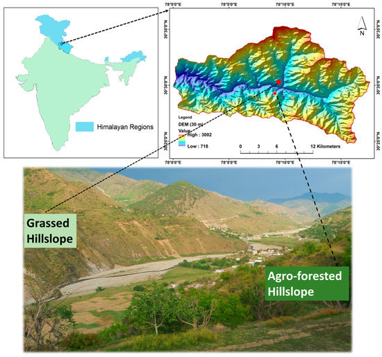
Figure 1.
Location of Aglar watershed in map of India; both aspects of watershed showing the location of grassed (GA) and agro-forested (AgF) hillslopes in Digital Elevation Model (DEM) (reproduced from Figure 1 of Nanda et al. [29] with the copyright permission from Elsevier office).
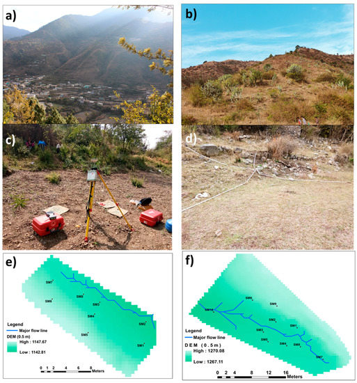
Figure 2.
(a) North aspect of watershed dominated with agricultural lands and forests; (b) south aspect of watershed dominated with bushes of Cactaceae family; (c) agro-forested hillslope during real-time kinematic (RTK) GPS survey; (d) grassed hillslope during soil moisture sensors installation; (e) 0.5 m resolution DEM of AgF hillslope showing major flow lines and locations of soil moisture; (f) 0.5 m resolution DEM of GA hillslope showing major flow lines and locations of soil moisture installation point (reproduced from Figure 1 of Nanda et al. [29] with the copyright permission from Elsevier office).
2.2. Hydrological Measurements
AgF and GA hillslopes were installed with hydrological and meteorological instruments. A 0.6-foot HS-flume with calibrated Odyssey capacitance based water level sensor (Dataflow system Ltd., Christchurch, New Zealand) was installed at the outlet of the hillslope for measuring the runoff generated during rainfall events. The runoff conversion of AgF hillslope was higher than the GA hillslope. At each hillslope, five Decagon (Meter Environment) and five Odyssey soil moisture sensors were installed horizontally at a depth of 15 cm from the surface to record fine-resolution (i.e., five min) soil–water dynamics. Spatial and temporal variations in soil temperature were also recorded at 5-min intervals using the same 5TM Decagon sensors. SM1, SM2, SM3, SM4, and SM5 sensor points have both soil moisture and soil temperature (−40 to +60 °C) data, whereas SM6, SM7, SM8, SM9, and SM10 sensors have only soil moisture data. In the present study, we only used the SM1–SM5 data points. RainWise tipping bucket rain gauges (RainWise Inc., Trenton, ME, USA) were instrumented near both hillslopes to measure the rainfall characteristics. Climate parameters were measured by automatic weather stations (AWSs). To understand the influence of rainfall and soil moisture on soil temperature dynamics, which is the part of the first research question of this paper, we analyzed 40 rainfall events of both hillslopes. The characteristics of selected rainfall events with corresponding changes in soil temperature and moisture are presented in Table 1 and Table 2 for GA and AgF hillslopes, respectively. The event duration of both hillslopes ranged between 1.17 h to 6.58 h.

Table 1.
Characteristics of selected rainfall events with corresponding changes in soil temperature and moisture in GA hillslope.
Table 2.
Characteristics of selected rainfall events with corresponding changes in soil temperature and moisture in AgF hillslope.
2.3. Training and Testing of the Model
To answer the second and third research questions, which are part of the soil temperature estimation, we used hourly and half-hourly time series data from 24 June 2017 to 5 April 2018 for all the meteorological parameters, rainfall, soil moisture, and soil temperature. Meteorological parameters included air temperature (Ta), solar radiation (Rs), relative humidity (RH), and vapor pressure deficit (VPD). VPD can be calculated using the given formula.
There was no need for normalization because there were no effects on an absolute scale. The database was divided into two parts: 75% for training and 25% for testing. Four different combinations of input variables were used for estimating soil temperature.
- Meteorological parameters (C1)
- Meteorological parameters + rainfall (C2)
- Meteorological parameters + soil moisture (C3)
- Meteorological parameters + rainfall + soil moisture (C4)
All the optimized parameters of each model are presented in Appendix A Table A1 and Table A2 for AgF and GA hillslopes, respectively.
2.4. Soil Temperature Estimation Algorithms
2.4.1. Multilayer Perceptron (MLP)
Multilayer perceptron (MLP) is a class of feedforward artificial neural networks. The name itself suggests that the multilayer perceptron consists of at least three layers of nodes: an input layer, a hidden layer, and an output layer [30]. Except for the input nodes, each node has a neuron that uses a non-linear activation function (ReLU, rectified linear unit). The hidden layers identify the complex relations between the input and output and in this present study, two hidden layers are taken. The number of neurons for each hidden layer was optimized between 2 to 100 by hit and trial approach for finding the best suitable neural network architecture. MLP utilizes the backpropagation learning algorithm to train the neural network model because of its robustness [31]. The detailed structure of MLP is presented in Appendix A Figure A1.
2.4.2. Random Forest (RF)
Random forests (RF) were proposed by Breiman [32] for establishing a predictor ensemble with a set of decision trees that grow in the randomly selected training data. In this algorithm, each of the trees is constructed using an injection of randomness, and the base constituents of the ensemble are tree-structured predictors; therefore, this procedure is called ‘random forests (RF)’ [33].
A random forest is a classifier function which is generated from a set of trees structured classifiers . These independent classifiers () are structured with the help of an ensemble of random vectors () and the training data (x). These random vectors consist of integer numbers between 1 and n. These integers in random vectors help in randomly splitting the training data and structuring the tree. By this procedure, a large set of trees is generated, and voting is done to select the most popular class. This whole process is called random forest.
Random forest models were tested for a different number of trees in the forest () and various combinations of maximum depth of the tree (). The value of varied between 10 to 100 and was allowed to expand until all leaves were pure or until all leaves contained less than in-sample-split samples for optimization of the model.
2.4.3. Support Vector Machine (SVM)
Support vector machine has become an increasingly useful tool for machine learning tasks involving classifications and regressions. It minimizes the structural risk to optimize performances on the training set [34]. The objective of a SVM is to establish the equation of a hyperplane that divides the training data leaving all the points of the same class on the same side in addition to the maximization of the minimum distance between either of the two classes and the hyperplane [35]. The equation of the hyperplane can be presented as
The two boundary line equations are
where +P and −P are the distances from the hyperplane, z represents set of predictors, and L is the hyperplane. Suppose the hyperplane is linear, i.e., in our case, the inequality satisfying the SVM will be
After trial and error, the linear kernel type is used in this study. The free parameters of the SVM model are C and epsilon. The parameter C regulates the balance between the loss function minimization (satisfying the constraints) and minimizing the regularization. The loss term that ignores errors within a certain distance of the true value is defined by epsilon [34].
2.4.4. Extreme Gradient Boosting (XGBoost)
Extreme gradient boosting system (XGBoost) is one of the most novel and versatile machine learning methods implemented by data scientists. The system runs more than 10 times faster than existing popular solutions on a single machine. XGBoost provides a parallel tree boosting (gradient boosting decision trees) that increases the speed and accuracy of the predictions [36]. XGBoost works on the principle of sequential tree building using parallelized implementation.
An initial model is built between the predictor and the target variable . Further, using the model , the simulated value yo is obtained. The residual is fitted with the new model . After that, the boosted version of the model (i.e., is obtained using both models and . The new residual is calculated from the newly simulated value using model . The residual model is obtained for . Now using and , another boosted model is obtained. It is important to note that each new boosted model will have a lesser mean squared error than its previous version. The iterative process of finding a new boosted model will stop when we reach the minima of residual error. The XGBoost model has two types of parameters: one guides the overall functioning, and the other booster parameter controls the regression at each step. The maximum tree depth () signifies the maximum tree depth for base learners and regulates the over-fitting of the parameters whereas minimum child weights () refer to the minimum sum of weights of all observations required in a child [37]. In addition to these two parameters, the maximum delta step () which is used to estimate the weight of each tree, is also taken into consideration for parameter optimization. The and were varied between 0 to 50, whereas was between 1 to 50.
All the models were analyzed in Python programming language packages. Scikit-learn, tensorflow, and xgboost packages [36,38,39] were used for analyzing RF and SVM, MLP and XGBoost models, respectively.
3. Results
3.1. Hillslope-Scale Soil Temperature and Moisture Variability
The spatial and temporal variability of soil temperature, soil moisture, and rainfall collected over 2017 water year (WY) is presented in Figure 3. Data gaps in soil moisture and temperature are due to the logger battery issue. The temporal rainfall variability of both hillslopes is almost the same. The maximum daily average rainfall depth of GA and AgF hillslope is 131 mm and 134 mm, respectively. The graph shows that the daily average soil temperature of the GA hillslope is more than the AgF hillslope as the south aspect hillslope (GA) receives more solar radiation than the north aspect (Figure 3). The seasonal variation in daily average soil temperature was between 6 °C to 27 °C in the AgF hillslope and 11 °C to 29 °C in the GA hillslope. The soil moisture started falling from the mid of September and the lowest spread is observed during colder months (i.e., November to February). During the warmer season, the soil moisture values are quite high. The runoff conversion of GA hillslope is less than the AgF hillslope which is also reflected in the spatial variability of soil moisture [29]. Thus, the GA hillslope shows more moisture content than the AgF hillslope. During monsoon season, daily average soil moisture values are above 0.15 m3/m3 for agro-forested (AgF) hillslope whereas for grassed (GA) hillslope, it was mostly above 0.20 m3/m3 (Figure 3). After the monsoon, soil moisture of both hillslopes reduced to 0.1 m3/m3.
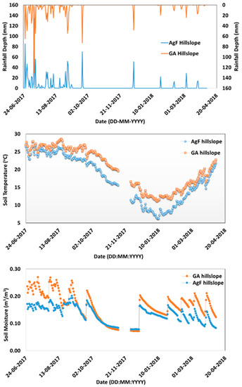
Figure 3.
Time series of rainfall, soil moisture, and soil temperature for AgF and GA hillslopes.
3.2. Influence of Rainfall on Soil Temperature
To analyze the influence of rainfall on soil temperature, the response of event scale (i.e., at 5-min resolution rainfall), for soil temperature, and moisture is shown in Figure 4 and Figure 5 for GA and AgF hillslope, respectively. It can be seen from Figure 4 that the high-intensity long-duration rainfall event of 26 June 2017 results in rapid drop of 3.3 °C in soil temperature whereas the high-intensity short-duration rainfall of 6 July 2017 event results in only a 1.5 °C fall in soil temperature of GA hillslope. Similarly, low- and medium-intensity long-duration rainfall events of 29 July 2017 and 31 August 2017 show 2.2 °C and 3 °C soil temperature drop, respectively. In the AgF hillslope, the drop in soil temperature was observed as 3.92 °C and 0.87 °C during high-intensity long (26 June 2017) and short (6 July 2017) duration events, respectively (Figure 5). Further, it is found that low- and medium-intensity rainfall of long duration results in a 1.99 °C temperature drop in AgF hillslope. Moreover, the soil moisture of high-intensity long-duration event of 26 June 2017 exhibits a 54.5% and 80.11% rise, whereas high-intensity short-duration rainfall of 6 July 2017 records a 36.7% and 28.19% rise in soil moisture in GA and AgF hillslope, respectively.
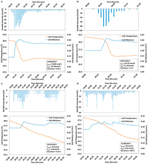
Figure 4.
Influence of rainfall on soil moisture and soil temperature dynamics in GA hillslope during four different rainfall events (a–d). The details about the rainfall events are mentioned in lower right corner of the plots.
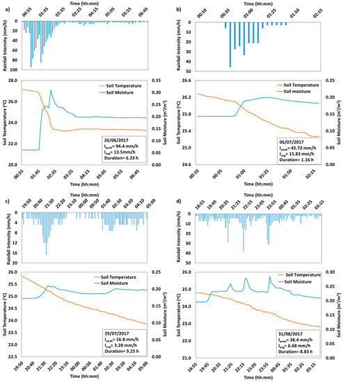
Figure 5.
Influence of rainfall on soil moisture and soil temperature dynamics in AgF hillslope during four different rainfall events (a–d). The details about the rainfall events are mentioned in lower right corner of the plots.
To understand these phenomena more clearly, the bubble graph [40] is plotted between event duration (h), event average rainfall intensity (mm/h), and drop in soil temperature in Figure 6. The significant drop in temperature is noticed during two situations, either when the rainfall duration is greater than 7.5 h or when the event average rainfall intensity is more than the 7.5 mm/h. The drop in soil temperature is less than 1 °C when the event duration and event average rainfall intensity is less than 7.5 h and 7.5 mm/h, respectively. Some expectations are also observed during the 6 July 2017 and 2 September 2017 rainfall events. The rainfall event on 6 July 2017 has a high average rainfall intensity but very short event duration (1.1 h) whereas the event on 2 September 2017 has a very low average rainfall intensity (<2.5 mm/h) with long event duration (>10 h). Thus, these two rainfall events show a very reduced drop in soil temperature even after exceeding the threshold value. It can also be observed that the short duration of winter rainfall was able to decrease the soil temperature significantly (>2 °C). For the similar average rainfall intensity and event duration condition, the temperature dropped by winter rain is higher than the monsoon rain. It is due to the freezing atmospheric temperature which affects the rainwater and soil temperature directly. Moreover, the drop in soil temperature is higher at the GA hillslope in comparison to the AgF hillslope which can be correlated with the amount of water infiltrated to each hillslope during rainfall events. The infiltration capacity of the GA hillslope is greater than the AgF hillslope. Further, we calculated the correlation between percentage changes in soil moisture and a drop in soil temperature (Figure 7). A significant correlation (p < 0.01) was found between these two variables with a coefficient value of 0.78 and 0.67 for GA and AgF hillslopes, respectively.
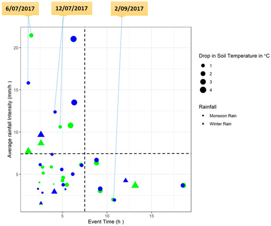
Figure 6.
Event duration (h) versus event average rainfall intensity (mm/h); size of the bubble shows the drop in temperature (°C); blue and green colors represent AgF and GA hillslopes, respectively.
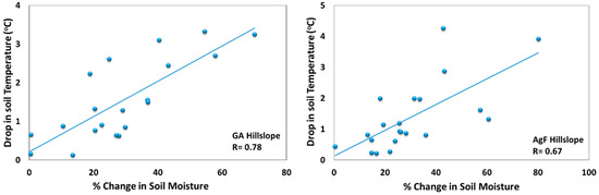
Figure 7.
Correlation between percentage changes in soil moisture and drop in soil temperature during each rainfall event of grassed (GA) and agro-forested (AgF) hillslopes.
3.3. Estimation of Soil Temperature at Half-Hourly and Hourly Scale
In this study, MLP, RF, SVM, and XGBoost models were used along with four different input combinations to create 16 different soil temperature estimation models for each time-scale and hillslope. Modeling of soil temperature for half-hourly and hourly scale was performed. The scatter plot between estimated and measured half-hourly soil temperature for the GA hillslope is presented in Figure 8. As presented in the figure, except for SVM, the other three models were able to capture the half-hourly soil temperature dynamics. Moreover, no improvement in soil temperature estimation was observed after adding rainfall components to meteorological inputs (Rs, Ta, RH, and VPD). Although a significant improvement in accuracy of soil temperature models was witnessed after using soil moisture along with the meteorological variables. The R2 value of MLP, RF, and XGBoost algorithm was found to be 0.859, 0.869, and 0.879, respectively for combination C1 (i.e., only meteorological); however, it was 0.953, 0.955, and 0.943, respectively for combination C3 (i.e., meteorological and soil moisture). The mean absolute error of MLP, RF, and XGBoost algorithm significantly reduced by 46.75%, 46.17%, and 37.5%, respectively after adding soil moisture to the meteorological inputs. For C1, XGBoost performed better than the MLP and RF algorithms. However, for C3, the RF model performed better than the MLP and XGBoost. The performance of hourly soil temperature estimation models for the GA hillslope is presented in Figure 9. Similar to the half-hourly results, it can also be seen from hourly regression plots that the efficiency of the SVM model is weaker than the MLP, RF, and XGBoost model. The significant improvement in model R2 from 0.864, 0.87, and 0.873 to 0.92, 0.924, and 0.965 was observed for MLP, RF, and XGBoost model, respectively after using soil moisture along with the meteorological data as an input parameter. XGBoost algorithm outperformed the remaining algorithms to estimate the hourly soil temperature of the GA hillslope for all the input combinations. For the AgF hillslope, the scatter plots of half-hourly and hourly soil temperatures are shown in Figure 10 and Figure 11, respectively. For C1 inputs which include pre-defined meteorological parameters, MLP, RF, SVM, and XGBoost algorithm were performed well to estimate half-hourly soil temperature with R2 values 0.919, 0.926, 0.831, and 0.932, respectively (Figure 10). In an hourly-scale, the XGBoost and RF algorithms (having R2 0.919 and 0.926, respectively) performed better than the SVM (0.834) and MLP (0.841). The efficiency of the XGBoost model is again found to be better than other studied models for both hourly and half-hourly soil temperature estimation of AgF hillslope. For both hourly and half-hourly soil temperature estimation, the C2 and C4 models did not show any significant improvement in the estimation of soil temperature after adding rainfall to C1 and C3 input combinations (Figure 10 and Figure 11). Although after adding only soil moisture to meteorological inputs, the R2 values of half-hourly and hourly algorithms raised significantly for AgF hillslope too. The mean absolute error (MAE) values dropped by 37%, 43.5%, and 46.37% in half-hourly MLP, RF, and XGBoost models after using C3 inputs compare to C1 inputs. Similarly, for the hourly scale, the MAE values of C3 models were reduced by 48%, 21%, and 33% in comparison to the C1 model for MLP, RF, and XGBoost algorithm, respectively.
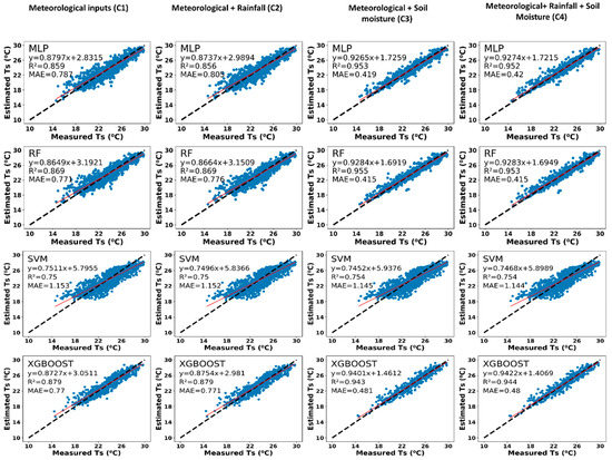
Figure 8.
Scatter plots between estimated and measured half-hourly soil temperature (Ts) showing R2 and mean absolute error (MAE) of 16 different model combinations for grassed hillslope (black dashed line represents 45 degree line and red solid line represents regression line).
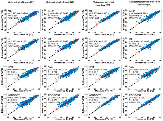
Figure 9.
Scatter plots between estimated and measured hourly soil temperature (Ts) showing R2 and MAE of 16 different model combinations for grassed hillslope (black dashed line represents 45 degree line and red solid line represents regression line).
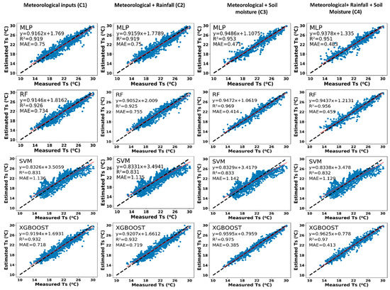
Figure 10.
Scatter plots between estimated and measured half-hourly soil temperature (Ts) showing R2 and MAE of 16 different model combinations for agro-forested hillslope (black dashed line represents 45 degree line and red solid line represents regression line).
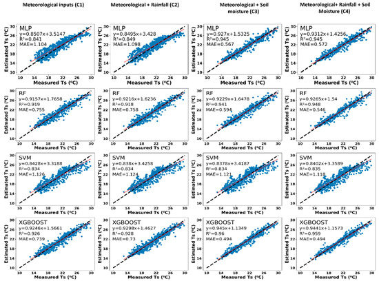
Figure 11.
Scatter plots between estimated and measured hourly soil temperature (Ts) showing R2 and MAE of 16 different model combinations for agro-forested hillslope (black dashed line represents 45 degree line, and the red solid line represents regression line).
4. Discussion
This study analyzed the influence of the hillslope aspect on soil temperature and the effect of rainfall duration and intensity on soil temperature dynamics using 40 rainfall events. In the present study, it was observed that the soil temperature of the south aspect hillslope (i.e., GA hillslope) was higher than the north aspect hillslope (i.e., AgF hillslope) as the south aspect receives more solar radiation than the north aspect. Kunkel et al. [3] also discussed the effect of site orientation on soil temperature in Krui, Stanley, and Merriwa watersheds. It was found that the soil temperature drop is linked with soil moisture rise, event duration, and event rainfall intensity. Zhi et al. [41] studied the effect of rainfall on soil moisture and soil temperature in active layers of the Qinghai–Tibetan Plateau. They also observed that water infiltration could influence the thermal dynamics of the active layers. The significant drop in soil temperature was noticed either when the average rainfall intensity exceeded the value of 7.5 mm/h or when the rainfall duration surpassed the value of 7.5 h.
In the second part of the paper, we used the time-series data of different combinations of the variable to predict the soil temperature on the hourly and half-hourly scale. The XGBoost machine learning algorithm performed better than the other machine learning algorithm to estimate the soil temperature of two lesser Himalayan hillslopes. The computational speed of the XGBoost model is better than the other machine learning models and the chance of overfitting is negligible in this model [42]. Fan et al. [42] compared the efficiency of XGBoost and SVM models for predicting global solar radiation and they found that the XGBoost model performed better and more efficiently than the SVM which was observed in the present study too. Moreover, Han et al. [43] studied the performance of XGBoost for the estimation of reference evapotranspiration using three weather stations of north China. They found that XGBoost outperformed the multivariate adaptive regression splines and the Gaussian process regression. Zhang et al. [26] used XGBoost model for simulating streamflow of the Qingliu River in limited data conditions and found satisfactory results. Gauch et al. [44] compared the data-driven model with a physical model to simulate the streamflow and they also observed that XGBoost performed better than the artificial neural network algorithm. Both of these studies corroborate with the results of the present study.
Similar to the XGBoost algorithm, RF outperformed the SVM and MLP models. Tyralis et al. [25] also discussed the good stability and better predictive performance of RF compared to other machine learning models. Moreover, RF can deal with the non-linear relation between dependent and predictor variables. In the present study, soil moisture and soil temperature were highly non-linearly correlated as the rise in soil moisture caused a decrease in soil temperature. Further, the RF model can handle small sample sizes better [25]. In this paper, a total of 4704 and 2352 data points were used for half-hourly and hourly model preparation, respectively. Out of the total number of data points 75% of data were used for training and the remaining 25% were used for testing. Proper care of the overfitting and underfitting was taken care of in the RF model. An increase in the depth of the tree causes overfitting while the number of trees causes underfitting of the data. Thus, both parameters were simultaneously optimized to prevent these issues. It was observed from all the scenarios that the MLP algorithm performed better than the SVM. Two hidden layers were used and a number of neurons in each layer were optimized manually in the range of 2 to 100 (Appendix A Table A1 and Table A2). Similar to our results, Tabari et al. [20] found that MLP can estimate daily soil temperature in arid climatic conditions. MLP is a type of ANN which is simple and effective and requires less variable comparisons for the analytical model for soil temperature estimation [17]. Surprisingly, SVM showed comparatively less accuracy in comparison to other machine learning models. The main cause of the low performance of SVM may be due to non-linearity among various analyzed variables. Raghavendra and Deka [23] discussed a major drawback of SVM that linearizes data on an implicit basis using kernel transformation which may be the reason for the low efficiency of SVM in this study. Furthermore, it will be worthwhile to discuss the limitations of this study. The primary limitation of the study is the limited availability of data. Various hydro-meteorological variables were available for 98 days; therefore, we could not conduct this study on a daily basis. However, with such minimal data three out of four machine learning models were able to capture soil temperature accurately.
Moreover, findings of this study show that the addition of rainfall data to meteorological (C1) or meteorological + soil moisture (C3) data results in a very negligible improvement in model accuracy which can be attributed to lesser data availability during the period of precipitation. Out of 2352 h of modeled data 93.13% of data were for no rainfall conditions. With fewer data points with precipitation, the machine learning model was not able to capture the effect of rainfall on soil temperature. Moreover, we expect that if we would have data for a few more years, the model can be trained only for the monsoon period data, then the inclusion of rainfall may provide better results. However, the addition of soil moisture data to meteorological parameters significantly improves the prediction results. Relative important metrics (Appendix A Figure A2) were prepared for all algorithms and a higher importance of soil moisture and the lesser importance of rainfall over other variables for predicting the soil temperature was observed. The importance of air temperature (Ta) was followed after the soil moisture (SM). Similarly, the importance of RH, Rs, and VPD was found to be less than the Ta, respectively. Bilgili [17] also mentioned the importance of considering soil moisture for soil temperature estimation especially in the regional forecast model. Depending on the different soil types, land cover, and rainfall variability, soil moisture shows very high spatial heterogeneity. While considering a small watershed, meteorological parameters may be in the same range over the landscape except for the soil temperature and moisture. Therefore, only by considering meteorological variables as predictor variables, one can predict the soil temperature of the observed point (for which model was prepared) but not for other points of the landscape. Especially in developing countries, installation of a large network of sensors is quite tough because of financial issues. The applicability of the developed model is possible in regions with hydrologic and meteorological similarity. However, for regions with the decision variables beyond the limit of the trained model, a retraining of the model may be necessary. Further, it was also observed that the addition of soil moisture to meteorological parameters significantly improved the soil temperature prediction. This proposed input parameter combination (meteorological + soil moisture) can be used in regional forecast models for predicting soil temperature. Moreover, this fine-resolution soil temperature model can be used as a decision making tool of precision agricultural systems. In addition, all of these models are point prediction models which can be extended for probabilistic predictions to show the uncertainty in prediction using an advanced statistical technique such as Gaussian process regression.
5. Conclusions
The soil temperature variability was studied in two Lesser Himalayan hillslopes. The soil temperature of the south aspect hillslope (i.e., the grassed (GA) hillslope), was 2 to 5 °C higher than the north aspect hillslope (AgF hillslope). The significant 2 °C soil temperature drop was observed either when the rainfall duration was greater than 7.5 h or event average rainfall intensity was greater than the 7.5 mm/h. Moreover, it was also observed that very high-intensity rainfall with very short event duration did not drop the temperature more than 1 °C. The higher infiltration capacity of the GA hillslope resulted in a higher drop in soil temperature in comparison to the AgF hillslope. During rainy days, the significant correlation (p < 0.01) was observed between soil moisture and soil temperature for both GA and AgF hillslopes having correlation values 0.78 and 0.67, respectively.
Among MLP, RF, SVM, and XGBoost machine learning algorithms, the XGBoost model performed best while the SVM model was the least performing model for both hourly and half-hourly scale. Soil temperature estimation efficiency of the RF algorithm was found to be better than the MLP algorithm. Moreover, the addition of rainfall to the meteorological inputs did not improve the efficiency of any discussed machine learning models. The addition of soil moisture to the meteorological parameters exhibited significant improvement in model performance and this combination was found to be the most efficient combination. The combination of three input variables (i.e., meteorological parameters, soil moisture, and rainfall) resulted in similar model efficiency as the meteorological and soil moisture inputs. The accurate estimation of soil temperature will be helpful for developing decision-support systems that can be utilized to investigate soil characteristics required for better crop yield.
Author Contributions
Conceptualization, A.N. and S.S.; methodology, A.N. and A.N.S.; software, A.N. and A.N.S.; validation, A.N. and A.N.S.; formal analysis, A.N. and A.N.S.; investigation, A.N. and A.N.S.; resources, S.S.; data curation, A.N.; writing—original draft preparation, A.N.; writing—review and editing, A.N., S.S., A.N.S., and K.P.S.; visualization, A.N. and A.N.S.; supervision, S.S.; project administration, S.S.; funding acquisition, S.S. All authors have read and agreed to the published version of the manuscript.
Funding
Authors would like to acknowledge the Science & Engineering Research Board (SERB), Department of Science and Technology (DST) under grant # SER-776 towards field visits and instrumentation. The authors are also grateful to editorial committee of Water, MDPI for providing 100% discount on Article Processing Charge (ACP).
Acknowledgments
The authors are grateful to all the members of the research group (especially Vikram Kumar and Ravi Meena) for their support during installation. Moreover, the authors are thankful to all the local field persons of Aglar watershed. The first author would like to thank the Ministry of Human Resource Development (MHRD), India for providing fellowship during the PhD program. The third author would like to thank the IIT Roorkee for providing SPARK summer internship to work under this project. Finally, authors would like to thank the anonymous reviewers for providing constructive comments and suggestions.
Conflicts of Interest
The authors declare no conflicts of interest.
Appendix A
Table A1.
Optimized model parameters of agro-forested (AgF) hillslope.
Table A1.
Optimized model parameters of agro-forested (AgF) hillslope.
| Algorithms | MLP (No. of Neurons) | RF | SVM | XGBoost | ||||
|---|---|---|---|---|---|---|---|---|
| Parameters | 1st Hidden Layer | 2nd Hidden Layer | Nest | Dmax | Epsilon | Dmax | Max Delta | Min W |
| Hourly | ||||||||
| C1 | 3 | 51 | 57 | 9 | 1 | 6 | 13 | 0 |
| C2 | 5 | 10 | 17 | 10 | 1 | 6 | 12 | 5 |
| C3 | 5 | 14 | 8 | 19 | 1 | 15 | 16 | 6 |
| C4 | 6 | 28 | 39 | 17 | 1 | 14 | 16 | 4 |
| Half-Hourly | ||||||||
| C1 | 3 | 43 | 17 | 11 | 1 | 6 | 9 | 12 |
| C2 | 5 | 41 | 16 | 9 | 1 | 6 | 9 | 10 |
| C3 | 5 | 56 | 18 | 16 | 1 | 15 | 10 | 4 |
| C4 | 6 | 85 | 13 | 17 | 1 | 19 | 0 | 4 |
Table A2.
Optimized model parameters of grassed (GA) hillslope.
Table A2.
Optimized model parameters of grassed (GA) hillslope.
| Algorithms | MLP | RF | SVM | XGBoost | ||||
|---|---|---|---|---|---|---|---|---|
| Parameters | 1st Hidden Layer | 2nd Hidden Layer | Nest | Dmax | Epsilon | Dmax | Max Delta | Min W |
| Hourly | ||||||||
| C1 | 3 | 5 | 19 | 8 | 0 | 4 | 11 | 1 |
| C2 | 4 | 6 | 17 | 11 | 1 | 4 | 10 | 2 |
| C3 | 2 | 8 | 15 | 18 | 1 | 12 | 11 | 2 |
| C4 | 2 | 5 | 14 | 17 | 0 | 11 | 11 | 2 |
| Half-Hourly | ||||||||
| C1 | 2 | 8 | 17 | 10 | 2 | 9 | 5 | 1 |
| C2 | 3 | 9 | 16 | 10 | 2 | 9 | 5 | 1 |
| C3 | 5 | 5 | 19 | 16 | 2 | 16 | 9 | 3 |
| C4 | 6 | 7 | 14 | 19 | 2 | 18 | 18 | 4 |

Figure A1.
The structure of MLP. Ta, RH, VPD, and SM are air temperature, relative humidity, vapor pressure deficit, and soil moisture respectively, representing input variables. Wij is the weight vector connecting the input and hidden nodes and βkl is the backpropagation weight between the output and input nodes.

Figure A2.
Relative importance metrics for predictor variables.
References
- Feng, Y.; Cui, N.; Hao, W.; Gao, L.; Gong, D. Estimation of soil temperature from meteorological data using different machine learning models. Geoderma 2019, 338, 67–77. [Google Scholar] [CrossRef]
- Hu, G.; Zhao, L.; Wu, X.; Li, R.; Wu, T.; Xie, C.; Qiao, Y.; Shi, J.; Cheng, G. An analytical model for estimating soil temperature profiles on the Qinghai-Tibet Plateau of China. J. Arid Land 2016, 8, 232–240. [Google Scholar] [CrossRef]
- Kunkel, V.; Wells, T.; Hancock, G.R. Soil temperature dynamics at the catchment scale. Geoderma 2016, 273, 32–44. [Google Scholar] [CrossRef]
- Wundram, D.; Pape, R.; Löffler, J. Alpine soil temperature variability at multiple scales. Arct. Antarct. Alp. Res. 2010, 42, 117–128. [Google Scholar] [CrossRef]
- Singh, S.K.; Pandey, C.B.; Sidhu, G.S.; Sarkar, D.; Sagar, R. Concentration and stock of carbon in the soils affected by land uses and climates in the western Himalaya, India. Catena 2011, 87, 78–89. [Google Scholar] [CrossRef]
- Blöschl, G.; Bierkens, M.F.P.; Chambel, A.; Cudennec, C.; Destouni, G.; Fiori, A.; Kirchner, J.W.; McDonnell, J.J.; Savenije, H.H.G.; Sivapalan, M.; et al. Twenty-three unsolved problems in hydrology (UPH)–a community perspective. Hydrol. Sci. J. 2019, 64, 1141–1158. [Google Scholar] [CrossRef]
- Qi, J.; Zhang, X.; Cosh, M.H. Modeling soil temperature in a temperate region: A comparison between empirical and physically based methods in SWAT. Ecol. Eng. 2019, 129, 134–143. [Google Scholar] [CrossRef]
- Martinez, C.; Hancock, G.R.; Wells, T.; Kalma, J.D. An assessment of the variability of soil temperature at the catchment scale. In MODSIM 2007 International Congress on Modeling and Simulation; Modeling & Simulation Society of Australia and New Zealand: Christchurch, New Zealand, 2007; pp. 2319–2325. [Google Scholar]
- Liang, L.L.; Riveros-Iregui, D.A.; Emanuel, R.E.; McGlynn, B.L. A simple framework to estimate distributed soil temperature from discrete air temperature measurements in data-scarce regions. J. Geophys. Res. Atmos. 2014, 119, 407–417. [Google Scholar] [CrossRef]
- Coleman, K.; Jenkinson, D.S.; Crocker, G.J.; Grace, P.R.; Klír, J.; Körschens, M.; Poulton, P.R.; Richter, D.D. Simulating trends in soil organic carbon in long-term experiments using RothC-26.3. Geoderma 1997, 81, 29–44. [Google Scholar] [CrossRef]
- Wells, T.; Hancock, G.R.; Dever, C.; Martinez, C. Application of RothPC-1 to soil carbon profiles in cracking soils under minimal till cultivation. Geoderma 2013, 207, 144–153. [Google Scholar] [CrossRef]
- Ni, J.; Cheng, Y.; Wang, Q.; Ng, C.W.W.; Garg, A. Effects of vegetation on soil temperature and water content: Field monitoring and numerical modelling. J. Hydrol. 2019, 571, 494–502. [Google Scholar] [CrossRef]
- Musie, M.; Sen, S.; Chaubey, I. Hydrologic Responses to Climate Variability and Human Activities in Lake Ziway Basin, Ethiopia. Water 2020, 12, 164. [Google Scholar] [CrossRef]
- Xing, L.; Li, L.; Gong, J.; Ren, C.; Liu, J.; Chen, H. Daily soil temperatures predictions for various climates in United States using data-driven model. Energy 2018, 160, 430–440. [Google Scholar] [CrossRef]
- Mihalakakou, G. On estimating soil surface temperature profiles. Energy Build. 2002, 34, 251–259. [Google Scholar] [CrossRef]
- George, R.K. Prediction of soil temperature by using artificial neural networks algorithms. Nonlinear Anal. Theory Methods Appl. 2001, 47, 1737–1748. [Google Scholar] [CrossRef]
- Bilgili, M. Prediction of soil temperature using regression and artificial neural network models. Meteorol. Atmos. Phys. 2010, 110, 59–70. [Google Scholar] [CrossRef]
- Zare Abyaneh, H.; Bayat Varkeshi, M.; Golmohammadi, G.; Mohammadi, K. Soil temperature estimation using an artificial neural network and co-active neuro-fuzzy inference system in two different climates. Arab. J. Geosci. 2016, 9, 377. [Google Scholar] [CrossRef]
- Mehdizadeh, S.; Behmanesh, J.; Khalili, K. Evaluating the performance of artificial intelligence methods for estimation of monthly mean soil temperature without using meteorological data. Environ. Earth Sci. 2017, 76, 325. [Google Scholar] [CrossRef]
- Tabari, H.; Sabziparvar, A.-A.; Ahmadi, M. Comparison of artificial neural network and multivariate linear regression methods for estimation of daily soil temperature in an arid region. Meteorol. Atmos. Phys. 2011, 110, 135–142. [Google Scholar] [CrossRef]
- Kim, S.; Singh, V.P. Modeling daily soil temperature using data-driven models and spatial distribution. Theor. Appl. Climatol. 2014, 118, 465–479. [Google Scholar] [CrossRef]
- Kisi, O.; Sanikhani, H.; Cobaner, M. Soil temperature modeling at different depths using neuro-fuzzy, neural network, and genetic programming techniques. Theor. Appl. Climatol. 2017, 129, 833–848. [Google Scholar] [CrossRef]
- Raghavendra, S.; Deka, P.C. Support vector machine applications in the field of hydrology: A review. Appl. Soft Comput. J. 2014, 19, 372–386. [Google Scholar] [CrossRef]
- Maier, H.R.; Jain, A.; Dandy, G.C.; Sudheer, K.P. Methods used for the development of neural networks for the prediction of water resource variables in river systems: Current status and future directions. Environ. Model. Softw. 2010, 25, 891–909. [Google Scholar] [CrossRef]
- Tyralis, H.; Papacharalampous, G.; Langousis, A. A brief review of random forests for water scientists and practitioners and their recent history in water resources. Water 2019, 11, 910. [Google Scholar] [CrossRef]
- Zhang, H.; Yang, Q.; Shao, J.; Wang, G. Dynamic streamflow simulation via online gradient-boosted regression tree. J. Hydrol. Eng. 2019, 24, 04019041. [Google Scholar] [CrossRef]
- Kumar, V.; Sen, S. Evaluation of spring discharge dynamics using recession curve analysis: A case study in data-scarce region, Lesser Himalayas. Sustain. Water Resour. Manag. 2017, 4, 539–557. [Google Scholar] [CrossRef]
- Nanda, A.; Sen, S.; Jirwan, V.; Sharma, A.; Kumar, V. Understanding plot-scale hydrology of Lesser Himalayan watershed—A field study and HYDRUS-2D modelling approach. Hydrol. Process. 2018, 32, 1254–1266. [Google Scholar] [CrossRef]
- Nanda, A.; Sen, S.; McNamara, J.P. How spatiotemporal variation of soil moisture can explain hydrological connectivity of infiltration-excess dominated hillslope: Observations from lesser Himalayan landscape. J. Hydrol. 2019, 579, 124146. [Google Scholar] [CrossRef]
- Hastie, T.; Tibshirani, R.; Friedman, J. The Elements of Statistical Learning The Elements of Statistical LearningData Mining, Inference, and Prediction, 2nd ed.; Springer: Berlin, Germany, 2009; ISBN 978-0-387-84858-7. [Google Scholar]
- Laxmi, R.R.; Kumar, A. Weather based forecasting model for crops yield using neural network approach. Stat. Appl. 2011, 9, 55–69. [Google Scholar]
- Breiman, L. Random forests. Mach. Learn. 2001, 45, 5–32. [Google Scholar] [CrossRef]
- Biau, G. Analysis of a random forests model. J. Mach. Learn. Res. 2012, 13, 1063–1095. [Google Scholar]
- Gill, M.K.; Asefa, T.; Kemblowski, M.W.; McKee, M. Soil moisture prediction using support vector machines. J. Am. Water Resour. Assoc. 2006, 42, 1033–1046. [Google Scholar] [CrossRef]
- Vapnik, V.N. The Nature of Statistical Learning Theory; Springer: New York, NY, USA, 1995; ISBN 978-1-4419-3160-3. [Google Scholar]
- Chen, T.; Guestrin, C. XGBoost: A scalable tree boosting system. In Proceedings of the ACM SIGKDD International Conference on Knowledge Discovery and Data Mining, Chicago, IL, USA, 3–17 August 2013; Volume 16, pp. 785–794. [Google Scholar]
- Chen, T.; He, T. xgboost: eXtreme Gradient Boosting. R Packag. version 0.4-2. 2015, Volume 1–4. Available online: http://cran.fhcrc.org/web/packages/xgboost/vignettes/xgboost.pdf (accessed on 30 December 2019).
- Pedregosa, F.; Varoquaux, G.; Gramfort, A.; Michel, V.; Thirion, B.; Grisel, O.; Blondel, M.; Prettenhofer, P.; Weiss, R.; Dubourg, V.; et al. Scikit-learn: Machine Learning in Python. J. Mach. Learn. Res. 2011, 12, 2825–2830. [Google Scholar]
- Abadi, M.; Barham, P.; Chen, J.; Chen, Z.; Davis, A.; Dean, J.; Devin, M.; Ghemawat, S.; Irving, G.; Isard, M.; et al. TensorFlow: A system for large-scale machine learning. In Proceedings of the 12th USENIX Symposium on Operating Systems Design and Implementation (OSDI), Savannah, GA, USA, 22 August 2016. [Google Scholar]
- Wickham, H. Ggplot2; Springer: New York, NY, USA, 2009. [Google Scholar]
- Wen, Z.; Niu, F.; Yu, Q.; Wang, D.; Feng, W.; Zheng, J. The role of rainfall in the thermal-moisture dynamics of the active layer at Beiluhe of Qinghai-Tibetan plateau. Environ. Earth Sci. 2014, 71, 1195–1204. [Google Scholar] [CrossRef]
- Fan, J.; Wang, X.; Wu, L.; Zhou, H.; Zhang, F.; Yu, X.; Lu, X.; Xiang, Y. Comparison of Support Vector Machine and Extreme Gradient Boosting for predicting daily global solar radiation using temperature and precipitation in humid subtropical climates: A case study in China. Energy Convers. Manag. 2018, 164, 102–111. [Google Scholar] [CrossRef]
- Han, Y.; Wu, J.; Zhai, B.; Pan, Y.; Huang, G.; Wu, L.; Zeng, W. Coupling a Bat Algorithm with XGBoost to Estimate Reference Evapotranspiration in the Arid and Semiarid Regions of China. Adv. Meteorol. 2019, 2019, 1–16. [Google Scholar] [CrossRef]
- Gauch, M.; Mai, J.; Shervan Gharari, J.L. Data-driven vs. physically-based streamflow prediction models. In Proceedings of the 9th International Workshop on Climate Informatics, Paris, France, 2–4 October 2019. [Google Scholar]
© 2020 by the authors. Licensee MDPI, Basel, Switzerland. This article is an open access article distributed under the terms and conditions of the Creative Commons Attribution (CC BY) license (http://creativecommons.org/licenses/by/4.0/).