Article

Hydrodynamic and Waves Response during Storm Surges on the Southern Brazilian Coast: A Hindcast Study

by
Andre de Souza de Lima
1,*,
Arslaan Khalid
2,
Tyler Will Miesse
2,
Felicio Cassalho
2,
Celso Ferreira
2,
Marinez Eymael Garcia Scherer
1 and
Jarbas Bonetti
1
1
Centro de Filosofia e Ciências Humanas, Programa de Pós-Graduação em Geografia, Departamento de Geociências, Federal University of Santa Catarina, Campus Universitário, Trindade, Florianópolis, SC 88040-970, Brazil
2
Department of Civil, Environmental, and Infrastructure Engineering, George Mason University, 4400 University Dr, Fairfax, VA 22030, USA
*
Author to whom correspondence should be addressed.
Water 2020, 12(12), 3538; https://doi.org/10.3390/w12123538
Submission received: 24 October 2020 / Revised: 23 November 2020 / Accepted: 28 November 2020 / Published: 16 December 2020
(This article belongs to the Special Issue Coastal Hazards Management)

Abstract

:
The Southern Brazilian Coast is highly susceptible to storm surges that often lead to coastal flooding and erosive processes, significantly impacting coastal communities. In addition, climate change is expected to result in expressive increases in wave heights due to more intense and frequent storms, which, in conjunction with sea-level rise (SLR), has the potential to exacerbate the impact of storm surges on coastal communities. The ability to predict and simulate such events provides a powerful tool for coastal risk reduction and adaptation. In this context, this study aims to investigate how accurately storm surge events can be simulated in the Southwest Atlantic Ocean employing the coupled ADCIRC+SWAN hydrodynamic and phase-averaged wave numerical modeling framework given the significant data scarcity constraints of the region. The model’s total water level (TWL) and significant wave height (Hs) outputs, driven by different sources of meteorological forcing, i.e., the Fifth Generation of ECMWF Atmospheric Reanalysis (ERA 5), the Climate Forecast System Version 2 (CFSv2), and the Global Forecast System (GFS), were validated for three recent storm events that affected the coast (2016, 2017, and 2019). In order to assess the potentially increasing storm surge impacts due to sea-level rise, a case study was implemented to locally evaluate the modeling approach using the most accurate model setup for two 2100 SLR projections (RCP 4.5 and 8.5). Despite a TWL underestimation in all sets of simulations, the CFSv2 model stood out as the most consistent meteorological forcing for the hindcasting of the storm surge and waves in the numerical model, with an RMSE range varying from 0.19 m to 0.37 m, and an RMSE of 0.56 m for Hs during the most significant event. ERA5 was highlighted as the second most accurate meteorological forcing, while adequately simulating the peak timings. The SLR study case demonstrated a possible increase of up to 82% in the TWL during the same event. Despite the limitations imposed by the lack of continuous and densely distributed observational data, as well as up to date topobathymetric datasets, the proposed framework was capable of expanding TWL and Hs information, previously available for a handful of gauge stations, to a spatially distributed and temporally unlimited scale. This more comprehensive understanding of such extreme events represents valuable knowledge for the potential implementation of more adequate coastal management and engineering practices for the Brazilian coastal zone, especially under changing climate conditions.

1. Introduction

Storm surges can lead to flooding and erosion in coastal environments and urbanized areas [1], significantly impacting the lives and economy of coastal communities [2]. These phenomena are mainly driven by the inverse barometer effect (i.e., atmospheric pressure) and the tangential wind stress over the free water surface [3]. Moreover, the combined effects of wind-generated waves and the gravitational forces that generate astronomical tides must also be considered to assess the total water level (TWL) amplitude during a storm surge event [4,5]. Although astronomical and meteorological tides are driven by fundamentally different processes, the TWL can be intensified if a storm surge co-occurs during spring tides. Timing, therefore, is also an important controlling factor on storm surges’ magnitudes and impacts, which are particularly more relevant in microtidal range regions [6,7]. As a representative case, the 2000 southernmost kilometers of the Brazilian coast are governed by a micro-tide regime, with a range lower than 2 m.
The Southern Brazilian Coast is highly susceptible to storm surges generated by extra-tropical cyclones and anticyclones that often cause water piling-up nearshore increasing wave action and, consequently, erosive processes [8,9]. According to [10] storm surges magnitudes’ in Southern Brazil can be 2 m higher than those observed on the Northern Brazilian coast. As a matter of fact, the state of Santa Catarina (27° S) in Brazil has been recurrently impacted by large events (i.e., events that exceed the usual magnitudes in the region) recently recorded in the southwest Atlantic Ocean. Hurricane Catarina (2004) was the first documented hurricane in South America, and made landfall as a category-1 hurricane, being responsible for approximately USD 163 million in damages [11,12]. During this major event, at least 45,000 homes were affected and more than 3700 people displaced, of which 40 were injured [13]. The frequency of such events also plays an important role in determining coastal vulnerability. For instance, between 1995 and 2014, an annual average of 28 meteorological events, which also include storm surges, impacted the state [11]. The events’ magnitude and frequency as well as their impacts may be aggravated given the projected climate changes [14].
As stated in the literature, the global mean sea level can rise from 0.52 to 0.98 m in 2100 [14]. In addition to the intrinsic damaging character of sea-level rise (SLR) itself, which has been intensively described by many climate change studies [15,16,17,18,19], significant increases in wave height due to more intense and frequent storms are expected in the Southern Ocean. Likewise, wave periods and directions might be also affected [14,20,21]. In this context of unprecedented changes and unobserved patterns, numerical models stand out as powerful tools to simulate such complex natural phenomena, either by means of historical hindcasting or simulating future scenarios [22]. Furthermore, it plays an important role in contributing to coastal management tools and strategies [23], such as the Brazilian Plan to Climate Change Adaptation at Coastal Zones and the Brazilian Program for Shoreline Conservation (ProCosta).
In Brazil, several hydrodynamic and wave models have been implemented since the 1980s to simulate the influence of the astronomical and meteorological components of the TWL [24], investigate the oceanic circulation in the continental shelf [25], investigate local tidal characteristics [26], evaluate coastal interventions, and understand local littoral processes [27], among others. However, a series of limitations must be highlighted, for example, the lack of precise coupled bathymetric and topographic surveys hampers the accurate representation of the surf zone and seafloor features in shallow waters, as well as the assessment of coastal flooding due to storm surges. Moreover, the poor network for ocean observation and the constant discontinuity in the available time series compromises its use for the model validation, as well as statistical analysis to identify patterns in meteorological events and their influence on ocean circulation [9,28,29]. This limitation in oceanographic data availability is typical in developing countries and has been widely reported in the literature [30,31,32]. Despite this limitation for numerical modeling implementation, the tightly coupled ADCIRC+SWAN hydrodynamic and phase-averaged wave models [33] have been recently employed in different poorly monitored areas to simulate water levels and waves during extreme events for coastal flooding studies. For instance, [34] showed a good agreement with observed data in a simulation of cyclone-induced storm surges in Bangladesh, based on a 900-m resolution bathymetry dataset. In India, [35] performed a satisfactory representation of extreme nearshore waves, which contributed approximately 30% of the TWL during an extreme event. The authors of [36] implemented a numerical model approach in Iran to assess the impacts of storm surges on coastal communities. In addition to data scarcity, the meteorological forcing component of storm surge simulation can also represent a model limitation, since it relies on estimations of the storm parameters based on available climate models [37].
Meteorological forcing (i.e., wind and pressure fields) represents a dominant mechanism that controls the storm surge magnitude. Therefore, model accuracy is critically related to the wind and pressure field’s input to the model setup [38]. Thus, it is expected that the proper implementation of a reliable hindcast or forecast storm surge system is highly dependent on meteorological inputs. However, such storm mechanisms are represented by an estimation of meteorological parameters coming from climate models. Hence, inherent uncertainties and specificities of each climate model must be taken into account, e.g., model resolution [39]. The models’ predictive skills were also extensively tested for storm surge simulation, considering the diverse range of available climate models that provide the necessary meteorological forces for the model implementation [40,41,42]. However, to the best of our knowledge, the ADCIRC+SWAN modeling approach has not been yet applied to the coastal areas of Brazil.
In this context, this study aims to understand how accurately storm surge events can be simulated in the Southwest Atlantic by implementing a numerical modeling approach in data-scarce areas. First, data availability regarding waves, TWL, astronomical tides, wind, and sea-level pressure were gathered for different temporal scale and spatial distribution. Next, three storm surge events were selected to implement the ADCIRC+SWAN model using three different meteorological forcing sources to investigate uncertainties in the wind and pressure fields, as well as the resulting TWL and waves in the Southwest Atlantic. Model outputs were validated against the available data and error metrics are presented to evaluate the model performance. Finally, a local scale study was developed in order to investigate two SLR scenarios. This manuscript is organized as follows. Section 2 presents the data availability for storm surge numerical models in the aforementioned study area, the model set-up, and the meteorological forcing specification. Section 3 presents the research results and discussion for the: (a) harmonic analyzes conducted to evaluate the model performance for astronomical tides prediction; (b) meteorological forcing validation for the selected events; (c) TWL simulation validation and error metrics; (d) waves validation and error metrics; (e) local scale application for different astronomical tides scenarios during storm surges, and Additionally, two SLR scenarios to exemplify the influence of different water elevation values nearshore. Section 4 provides the conclusions.

2. Materials and Methods
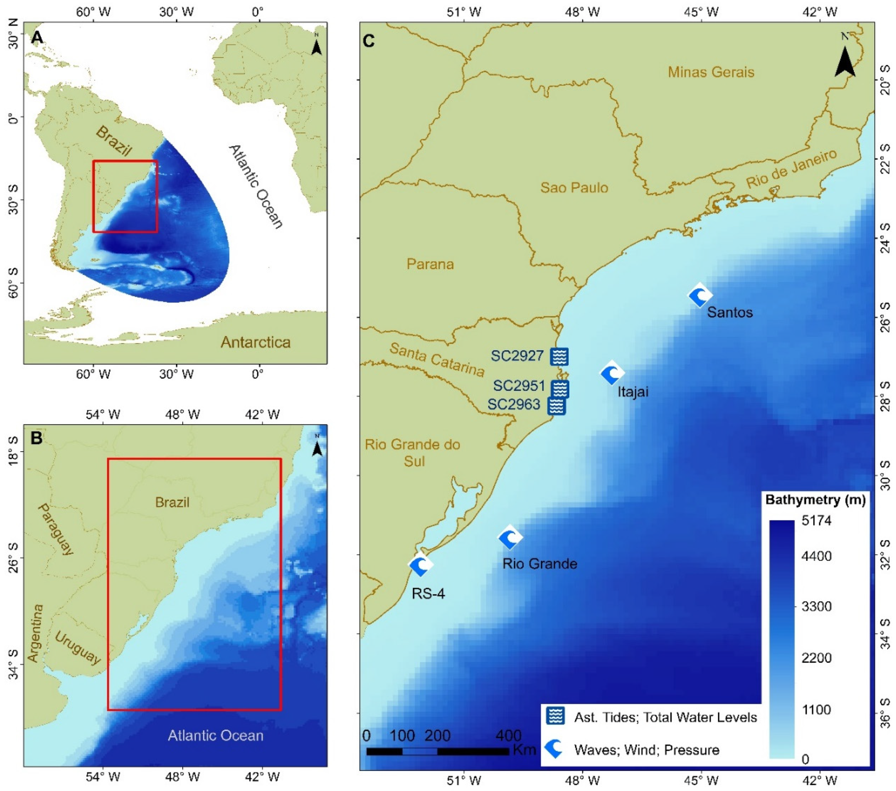
2.1. Study Area

Our study area encompasses the entire Southern Brazilian continental shelf, which extends from 22° S to 34° S throughout approximately 34% of the Brazilian coast, where the South and Southeast administrative regions are situated (Figure 1C). These regions concentrate the most densely populated and heavily industrialized areas of that coastal zone and have a significant influence on the country’s economy. In addition, the area converges the five most important Brazilian seaports, including the Port of Santos, which is the busiest container port in Latin America [43]. The area is predominantly characterized by a humid subtropical climate and a large variety of coastal and marine ecosystems, such as sandy beaches, mangroves, and coastal lagoons [44], which has turned it into a popular tourist destination. Regarding the regional oceanographic characteristics, the continental shelf circulation is influenced by oscillations of the Subtropical Shelf Front (confluence of Brazil and Malvinas currents), located near 33° S, as well as by the northwards transport close to the coast of low salinity waters from the La Plata River and the Patos/Mirim system [45]. Based on available wave data, [46] indicated that the predominant wave directions in the Southern Brazilian continental shelf are 100° and 160° (E–SE), while the wave heights vary from 1 to 1.5 m. Regarding the wave period, a variation between 6 and 14 s was observed. Although winter is the most energetic season on the Southern Brazilian coast, big waves (i.e., significant wave height (Hs) higher than 4 m) are present in all seasons [47]. Furthermore, despite its microtidal regime, the maximum values of both Hs and storm surge on the Brazilian coast are found in this region due to its high exposure to frequent and intense extratropical storms [9,10].
According to [48], the Southwest Atlantic Ocean presents two centers of cyclo-genesis along the Uruguay coast (35° S) and San Matias Gulf in Argentina (40° S), with higher frequency during winter and increased baroclinic instability during El Niño years. In a more recent study, three cyclogenesis regions were identified in the Southwest Atlantic Ocean, located in the Southern Brazilian coast (30° S), La Plata river discharge region, in Uruguay (35° S), and the Southern coast of Argentina (40° S–55° S) [49]. In addition, [50] highlighted that the Southern Brazilian coast is also susceptible to high-pressure fields known as anticyclones genetic regions at around 30° S, which have a major influence on the regional atmospheric circulation. However, according to [51], cyclones are the main weather system, responsible for 87.1% of extreme winds occurrence on the Southern Brazilian coast. Despite the main regional atmospheric patterns, the sub-synoptic-scale and local characteristics have an important role in events intensification [50]. Thus, the high susceptibility to storm surge events, along with a densely populated coastal zone, favors a high vulnerability status to the coastal communities in the study area [52].

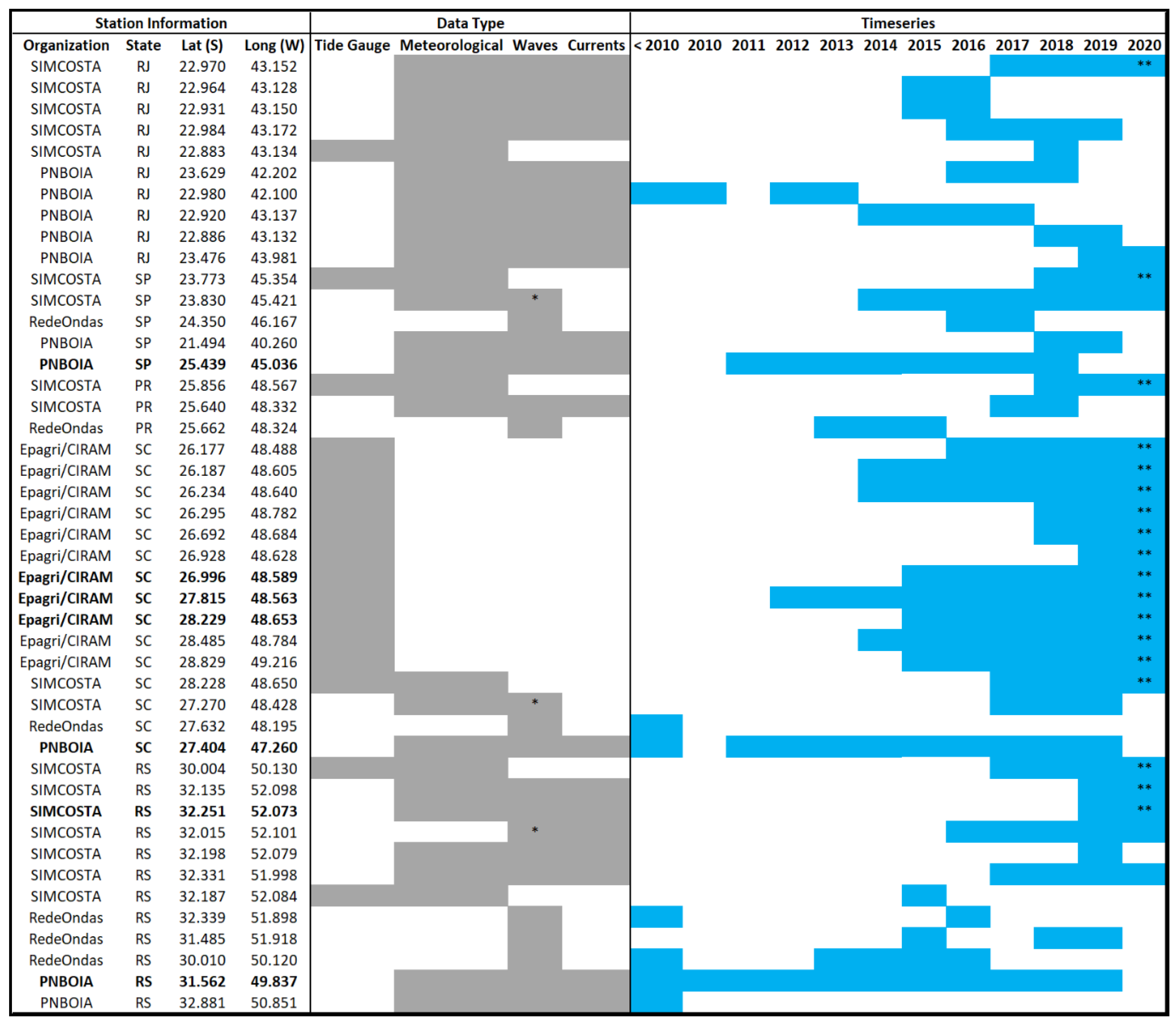
2.2. Data Availability

Figure 2 presents the data availability for the Southern Brazilian coast considering its five different coastal states for the last 10 years. Brazil also has tidal observational data throughout its coastline acquired by its ports and specific academic projects that gather ocean data for short periods (i.e., weeks, months). However, data are often unavailable for third parties and/or are not interoperable. Although meteorological data are made available for long periods (i.e., almost a century), such as the time series provided by the Brazilian National Meteorology Institute (INMET), stations are often located overland, making it difficult to use for hydrodynamic modeling validation.
Data discontinuity is evident throughout the time series. The period between 2018 and 2019 presents the highest number of operational stations. Nevertheless, none of the stations gathered data for the entire analyzed 10 years period. Furthermore, wave buoys present several gaps and/or equipment noises. At this moment, the study area encompasses 18 operational stations, including three wave buoys and 15 tide gauges (Figure 2).
Given the context of this scarce observational data, only three different storm surge events were selected between 2016 and 2019 based on waves and TWL available data for model validation. All selected events presented major TWLs in the station records and were related to distinct astronomical tidal cycle characteristics. The first event occurred in October 2016 (Storm 1) with a duration of three days, in spring tide condition. The second event occurred in May 2017 (Storm 2) with a duration of two days in the neap tide. Finally, the third event occurred in July 2019 (Storm 3) with a duration of 7 days also during a spring tide. Figure 1 shows both the numerical modeling domain (A) and the selected stations and buoys for model validation (C).

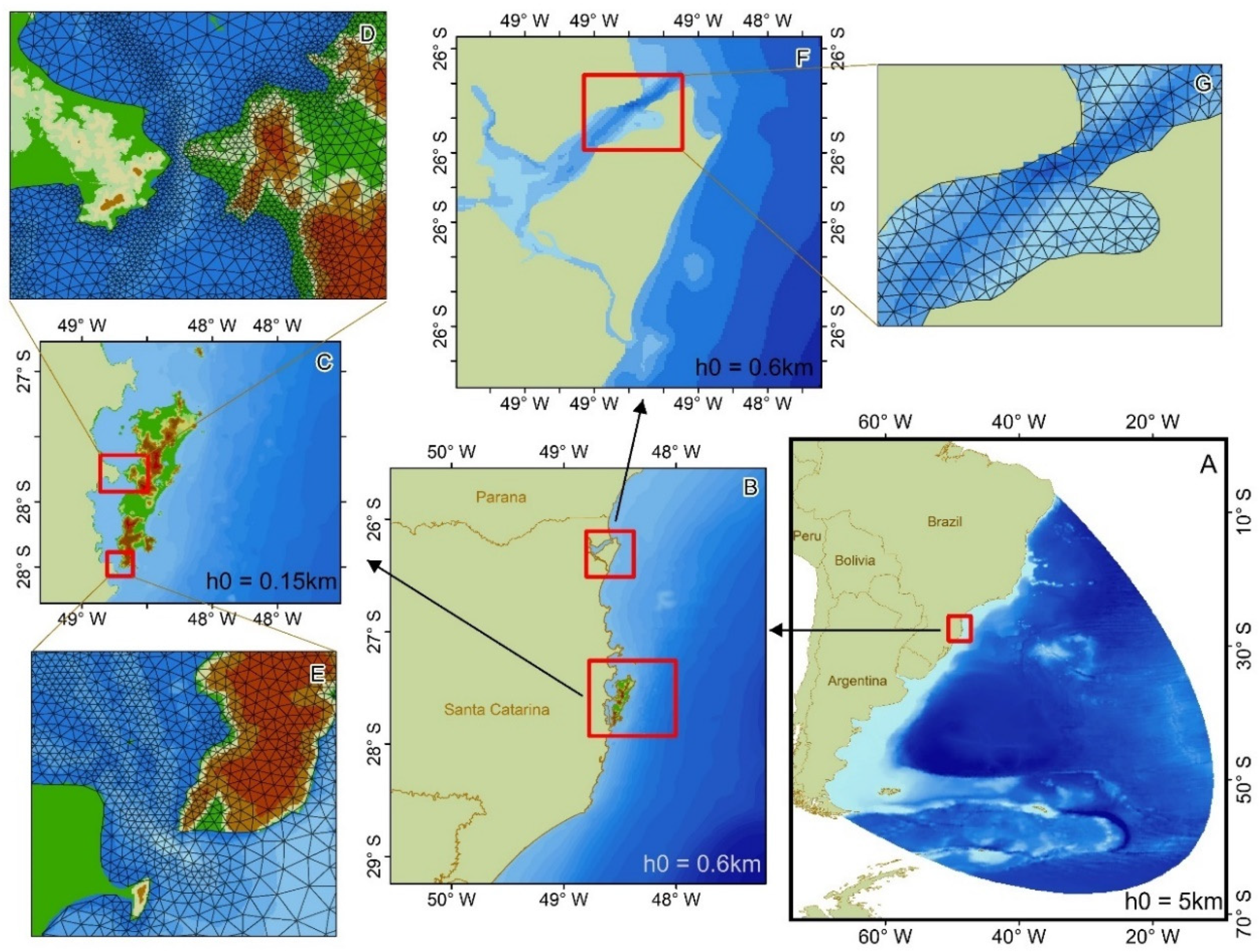
2.3. Modeling Approach

In the present study, the tightly coupled ADCIRC+SWAN hydrodynamic and phase-averaged models [33] were employed to simulate the evolution of the storm surge and the propagation of wind-generated waves from the open ocean to the coastal areas in order to assess and validate the TWL during three different meteorological events. In this context, for this study, the TWL results from the combined effects of astronomical tides, meteorological tides, and wave set-up [53]. Despite the fact that this numerical modeling approach has been applied to several studies in different parts of the world [34,54,55,56], it has not been previously applied in Brazil.
The ADvanced CIRCulation (ADCIRC-2DDI) model is a two-dimensional depth-integrated, finite-element-based hydrodynamic model based on the generalized wave continuity equation (GWCE) and depth-averaged momentum equations [57]. ADCIRC is one of the most commonly used hydrodynamic models for coastal flooding simulations as well as for astronomical tides, storm surges, and TWL worldwide [55,58,59,60]. The Simulating WAves Nearshore (SWAN), on the other hand, is a third-generation phase-averaged spectral wave model [61] that is applied to solve the wave action balance equation to obtain wave parameters in the numerical domain. Furthermore, in order to represent the resistance between hydrodynamic and wave interaction, and different surfaces and/or obstructions, landcover classes are treated as an enhanced bottom friction value (Figure 3C), i.e., different Manning’s n coefficients are selected according to each landcover class [62,63] and converted into a friction length in the model domain [64].
In a coupled mode, ADCIRC+SWAN can share both the same unstructured numerical mesh and parallel computing infrastructure, allowing the model components to be applied at the same time. In this modeling setup, the time step for ADCIRC is set to 1 s, while for SWAN the time step is set to 3600 s to maintain computational stability. According to [33], SWAN accesses wind speed, water levels, and currents provided by ADCIRC to compute radiation stress gradients that allow ADCIRC to re-calculate set-up and currents. Subsequently, SWAN uses this information to recalculate water depth and wave related parameters (i.e., propagation, breaking, etc.) that will update ADCIRC again as a forcing function. Note that SWAN does not calculate infragravity waves and wave run-up.
The model domain was designed to incorporate all meteorological specificities that might influence the study area such as spatial distribution and frequency of cyclogenesis in the Southwest Atlantic Ocean pointed out by [48,49,50]. Figure 3 presents the mesh domain and its different resolution ranges along the Southern Brazilian coast.
With a total of 116,695 nodes and 229,904 triangular elements, the grid resolution varies from 25 km in the open ocean boundary (Figure 3A) to 30 m along the Santa Catarina Island, where the only area overland was conceived in order to allow the local scale scenario analyses (Figure 3C). The two-dimensional unstructured mesh generation process was carried out via OceanMesh2D, an objected-oriented framework [65]. The mesh resolution was distributed in several nested boxes, allowing high resolution in the study area. Different minimum mesh sizes (h0) are shown in Figure 3, as well as the thalweg mesh size function (Figure 3B,D) that was enabled to improve water conveyance nearshore. Regarding the geographic database, the General Bathymetric Chart of the Oceans (GEBCO) [66] with a 15 arc-second of grid resolution was employed here in addition to nautical charts from the Brazilian Navy [27], used only for the center part of Santa Catarina State at depths lower than 50 m. In order to characterize the topography of Santa Catarina Island, utilized in the scenario analyses (presented in Section 2.5), the Secretaria de Estado do Desenvolvimento Economico Sustentavel (SDS) Digital Elevation Model was employed [67]. Additionally, as a means to characterize the coastline geometry, the Global Self-consistent, Hierarchical, High-resolution Geography Database [68] was utilized. All nearshore topobathymetric data have been standardized to the Mean Sea Level (MSL) of the local vertical datum.

2.4. Hindcast Parameters

For each selected storm surge event, data from three different meteorological forcing sources were used to assess model sensitivity regarding different climate model specificities. The fifth-generation ECMWF atmospheric reanalysis (ERA5) [69], which has a grid resolution of 0.25° × 0.25°, the Global Forecast System (GFS) [70], with a spatial resolution of 0.5° × 0.5° and, finally, the Climate Forecast System Version 2 (CFSv2) [71], which is presented in a 0.2045° × 0.2045° grid, were all considered as the main wind and pressure forcing of the model setup. Both winds at 10 m above the sea surface and mean sea level pressure were extracted from the aforementioned climate models to perform the hydrodynamic and wave simulations on intervals of 6 h.
The numerical modeling simulations were performed with open boundaries using a forcing of 12 harmonic tidal constituents (M2, S2, O1, K1, K2, N2, Q1, M4, P1, 2N2, MS4, MN4) derived from TPXO 9.1 [72]. However, to accurately represent the astronomical tides in our domain, a 4-month tide-only simulation (starting on 1 September 2019) was carried out using the ADCIRC standalone model. The harmonic analysis was performed for the last 90 days of the simulation [73] as well as the form number calculation to estimate the regional tidal type [74]. Constituents amplitudes were validated against the Epagri/CIRAM predictions during the same period.
Understanding uncertainties and errors associated with the numerical approach is also an important factor for planning and mitigation actions in the coastal zone [75]. Thus, model performance was analyzed comparing model outputs (i.e., both wind and pressure fields, TWL, astronomical tides, and Hs) against tide gauges and wave buoys observed data. The performance was quantified using the root-mean-square error (RMSE) [76] for TWL, astronomical tides, and Hs. Wind and pressure fields are qualitatively discussed in Section 3.2.

2.5. Scenarios Analysis

The analysis of the three scenarios are presented in the last section of this manuscript. We simulated Storm 1, which occurred in October 2016 during a spring tide cycle, under a different astronomical forcing, to verify the TWL for the same meteorological conditions during the neap tide and, therefore, verify the dependency among the two storm-surge main forcing parameters. Moreover, the same meteorological event was also simulated under two different SLR scenarios pointed out by the IPCC’s Fifth Assessment Report (AR5) in two different Representative Concentration Pathways (RCPs 4.5 and 8.5) as a global mean SLR in 2100, i.e., the far horizon for the global SLR scenarios [14]. The results were discussed within our modeling domain, focused on a local scale cutout in Ingleses Beach, located in the northeast of the Santa Catarina Island, Florianopolis. The selected area is a tourist destination and presents both natural and dense urbanized coastlines that have had recent problems with severe erosion due to storm surges [8].

3. Results and Discussion

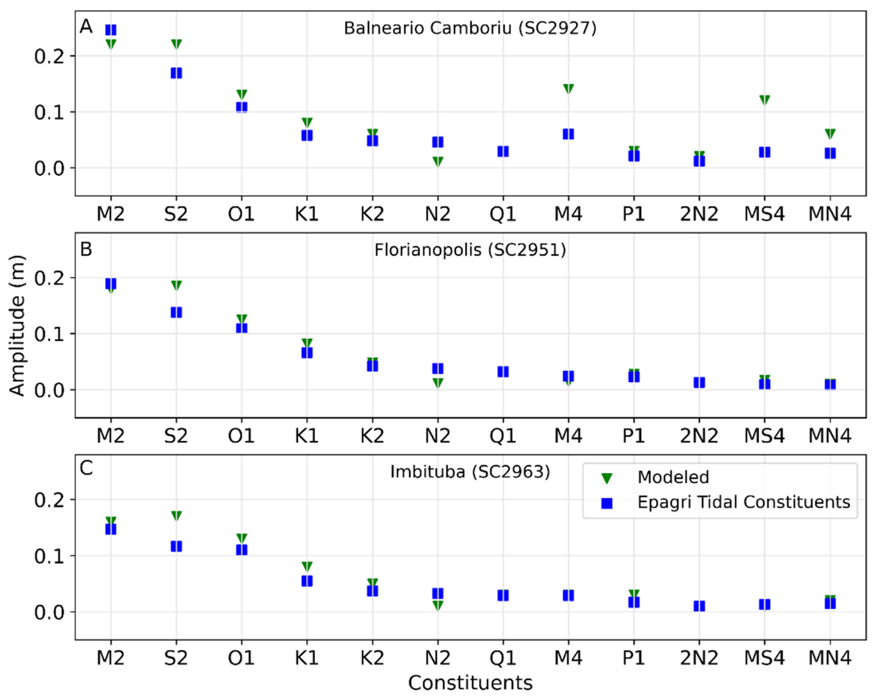
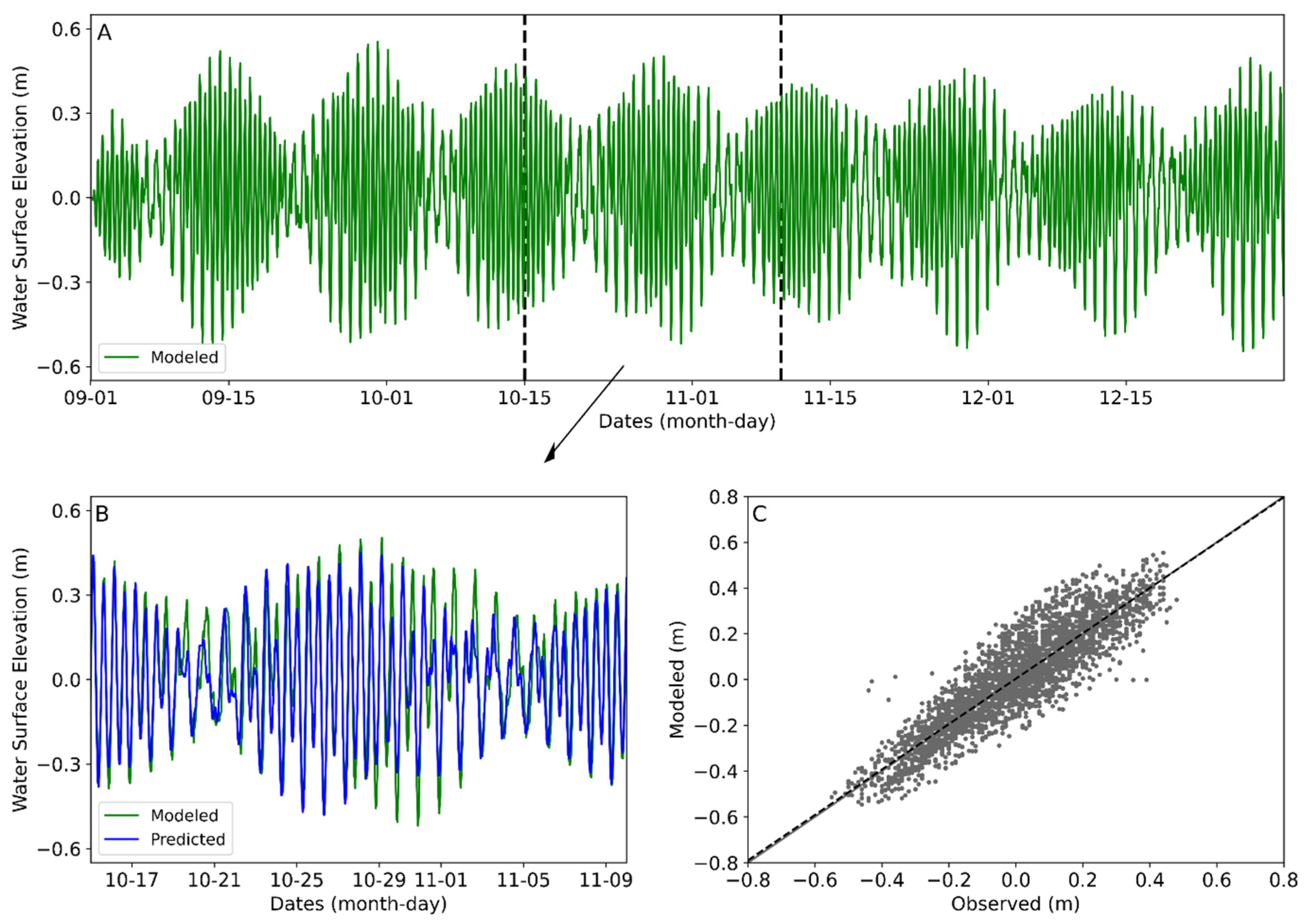
3.1. Astronomical Tides

The harmonic analysis was carried out for a period of four months, and the results were compared against astronomical tidal predictions in three stations in the Santa Catarina State. The sector analyzed presents a mixed, semidiurnal microtidal type, i.e., two unequal high tides and two unequal low tides, presenting form numbers between 0.25 and 1.5. The results of the harmonic analysis regarding constituents’ amplitudes are presented in Figure 4, while phases are shown in the supplementary material (Figure S1). The ADCIRC model was able to accurately represent all major harmonic constituents aside from M4 and MS4 at the northernmost station (Figure 4A). Moreover, the S2 constituent was responsible for generating the largest residual errors at all analyzed stations. For instance, at the Florianopolis station (SC2951), S2 was overestimated by 0.047 m, while M2 was underestimated by 0.009 m.
The time series presented in Figure 5A refers to the entire simulation period at the Florianopolis station (SC2951), where the calculated RMSE is 0.10 m. On the other hand, the Balneario Camboriu Station (SC2927) and Imbituba station (SC2963) present an RMSE of 0.24 and 0.11 m, respectively. Figure 5B highlights, in detail, the low amplitudes of a mixed, semidiurnal microtidal type as well as a misrepresentation of the transitions between spring and neap tides. However, as depicted in Figure 5C, a strong dependence is evident between the observed and modeled values, showing a suitable representation of astronomical tides.
According to [77], the third-diurnal principal lunar constituent (M3) has a significative amplitude in our study area and its resonance directly affects the astronomical tides signal. For instance, although the predictions present amplitudes up to 0.038 m for the M3 constituent in Balneario Camboriu station, the tidal database TPXO 9.1 [72] has no tidal data for the aforementioned constituent. Additionally, the lack of a precise and up to date bathymetry and its relative importance for an appropriate hydrodynamic simulation must be emphasized [78].

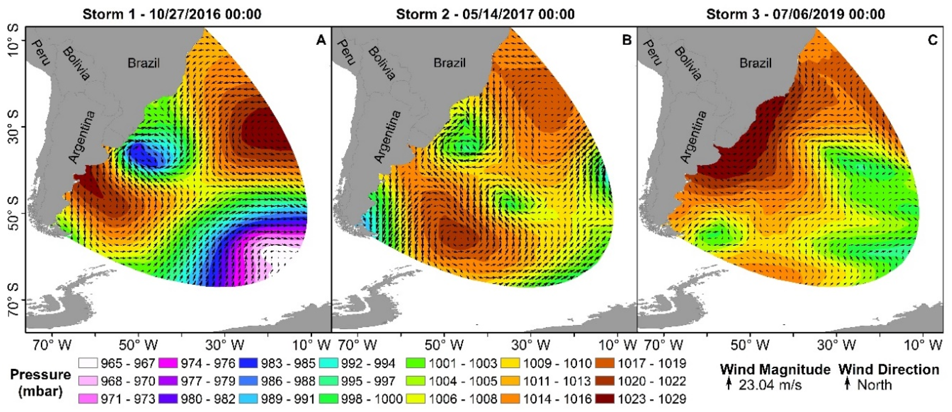
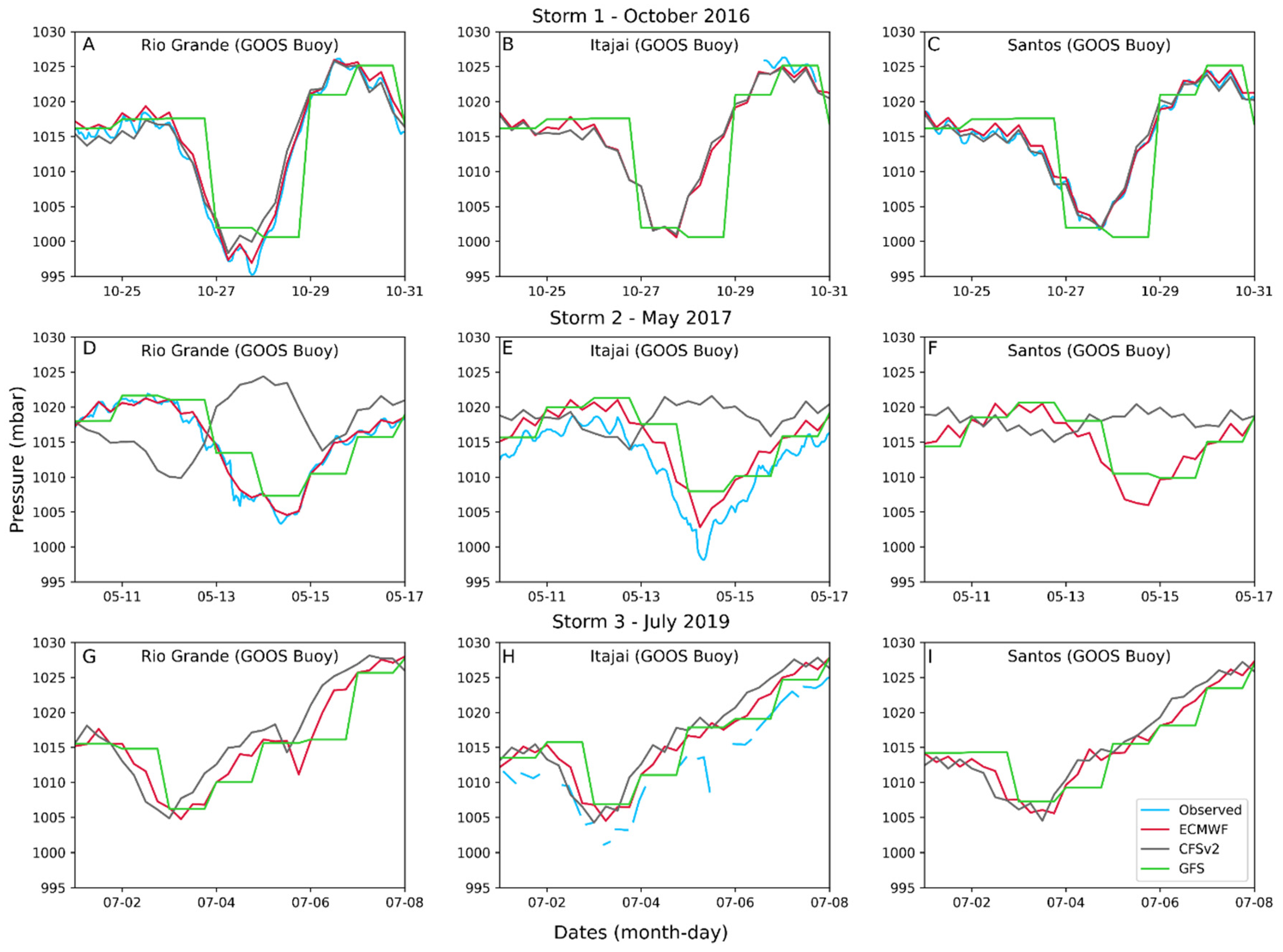
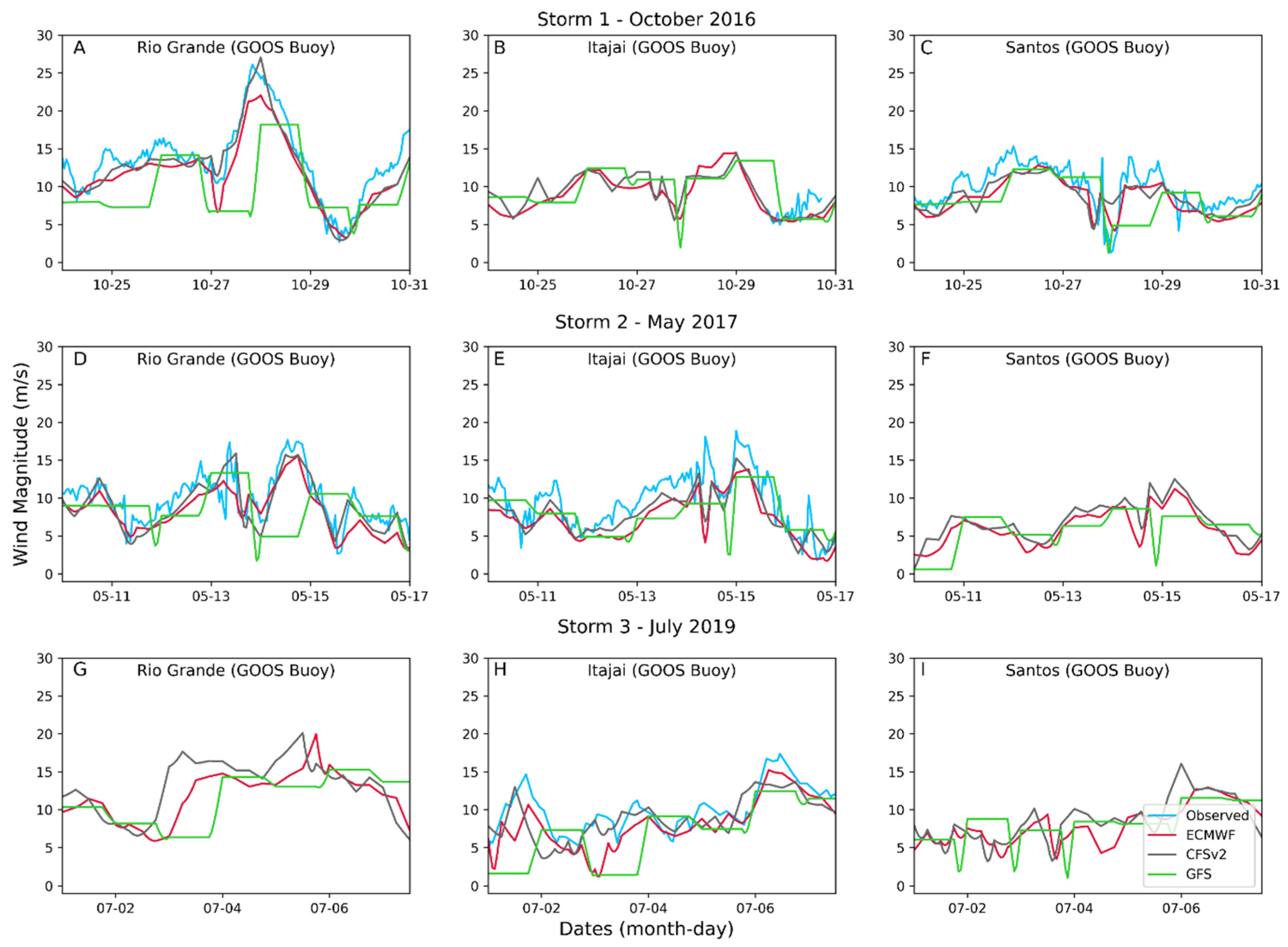
3.2. Wind and Pressure Fields

Figure 6 depicts both wind and pressure fields in the model domain for three specific dates representing the atmospheric conditions when the TWL peaks were recorded at the tide gauges in Santa Catarina. Both Storm 1, which occurred during spring (Figure 6A), and Storm 2, which occurred in the fall (Figure 6B), were generated by extra-tropical cyclones with similar spatial and atmospheric conditions. On the contrary, Storm 3, which also occurred in the fall, was generated by a high-pressure field adjacent to the coast (Figure 6C). Due to different climate model resolutions and a lack of observation data, both wind and pressure fields were qualitatively analyzed in three different buoys (Figure 1).
During Storm 1, all three climate models were able to characterize the time-series variation regarding the air pressure at mean sea level (Figure 7A–C). However, as a probable consequence of its coarser resolution, the GFS model was not able to represent the low-pressure peak (Figure 7A) as well as small variations throughout the time series. In contrast, although having a better resolution, the CFSv2 model completely misrepresented the pressure variations during Storm 2 (Figure 7D–F). None of the climate models were able to accurately represent the low-pressure peak at the closest buoy to the Santa Catarina state coastal zone (Figure 7E). Finally, in Storm 3, all climate models presented a suitable representation of pressure amplitudes with a slight shift in the phase if compared with the observations (Figure 7H).
The tangential wind stress is a dominant variable of a meteorological event and its action over the sea surface can represent up to 90% of a storm surge magnitude [79]. Regarding the climate models’ performance, both ECMWF and CFSv2 were able to represent wind magnitude amplitudes throughout the time series. The GFS model, on the contrary, consistently underestimated wind magnitudes and did not accurately characterize the high peaks observed in the Rio Grande buoy (Figure 8A,D) and Itajai buoy (Figure 8E). As in the pressure data, a slight shift in the phase can be observed under a high-pressure event (Figure 8G).
Although seemingly distant, the observed and modeled wind data in the southernmost buoy (Figure 8A,D,G) are still related to the meteorological monitoring conducted in the Rio Grande do Sul coast. [50] obtained maximum wind magnitudes of 24 m/s, and [51] found an average wind magnitude of 6.2 m/s and maximum values of 26 m/s over 66 years of storm surge analysis. Through a distribution analysis, all wind magnitudes higher than 17 m/s were classified as extreme winds, which occurred only in 0.16% of the observed data time series [51].

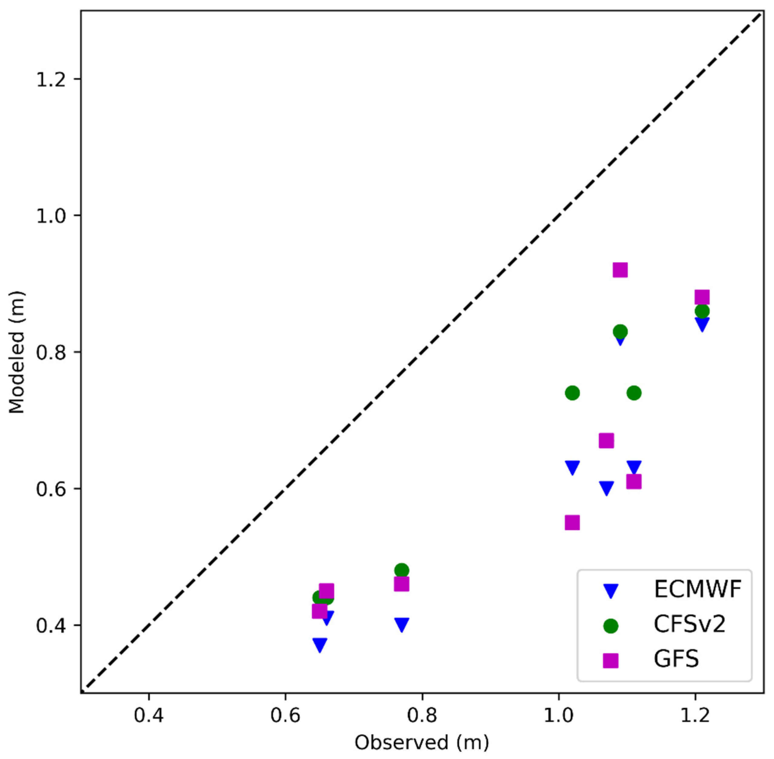
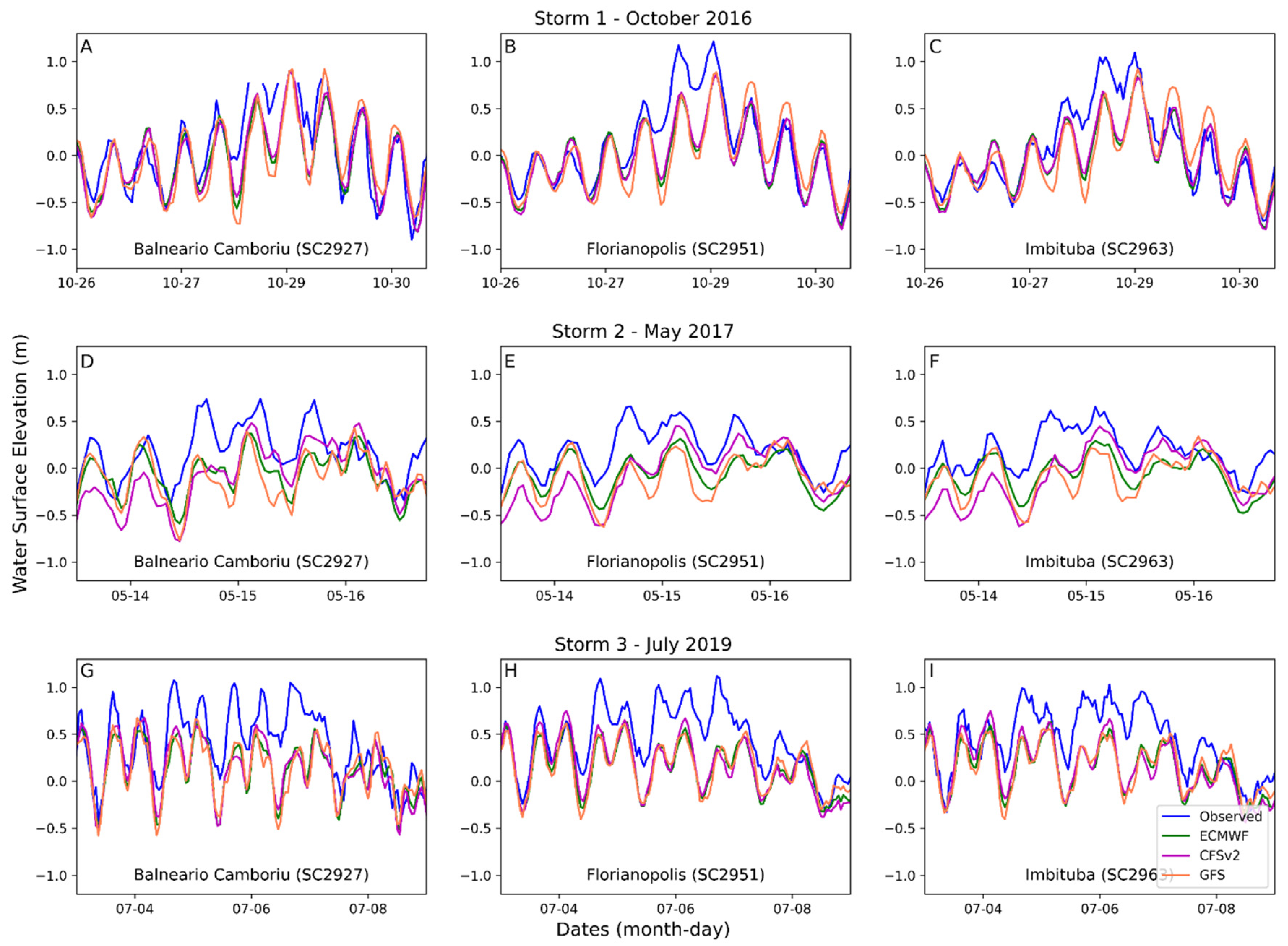
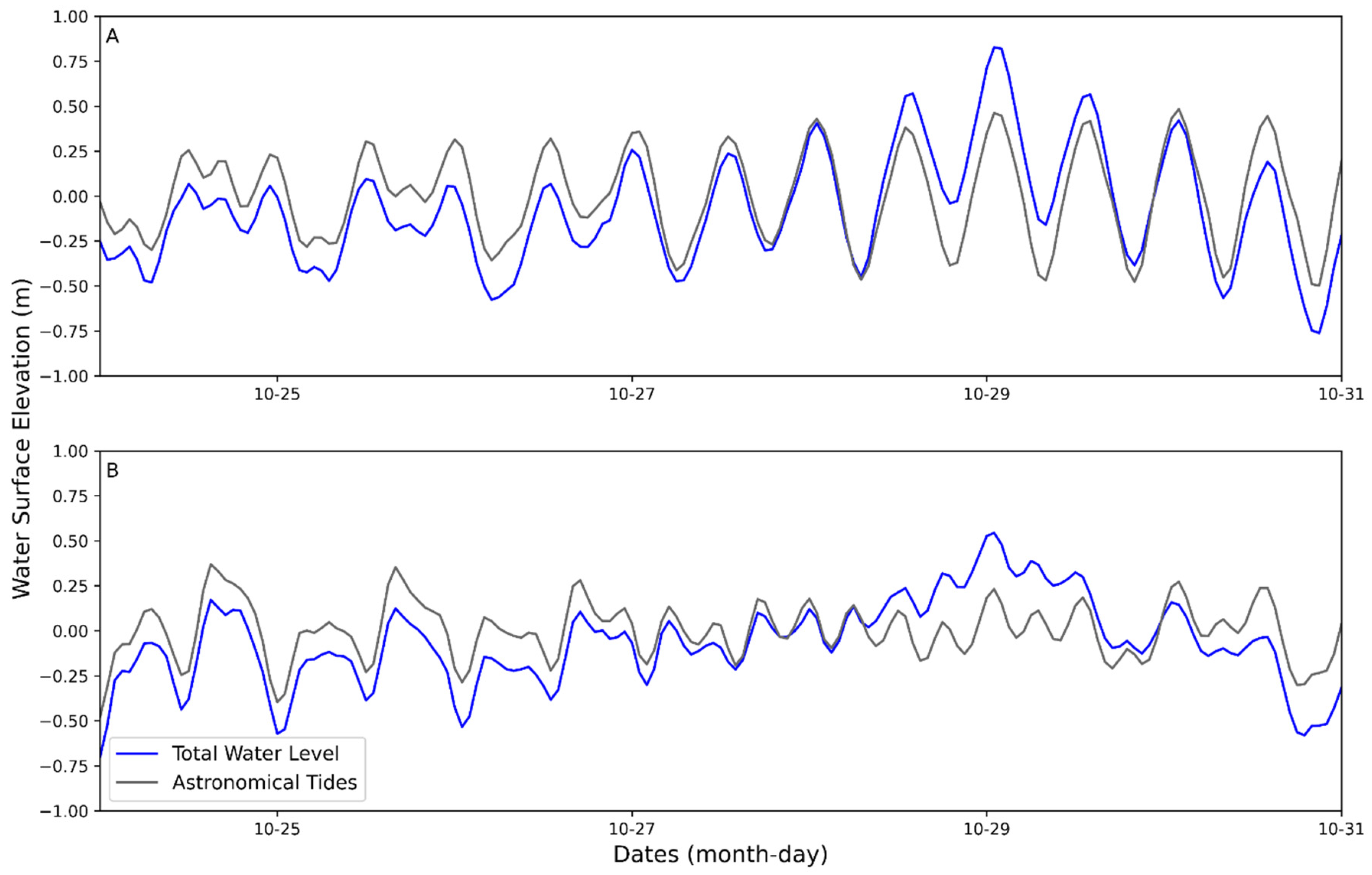
3.3. Total Water Levels
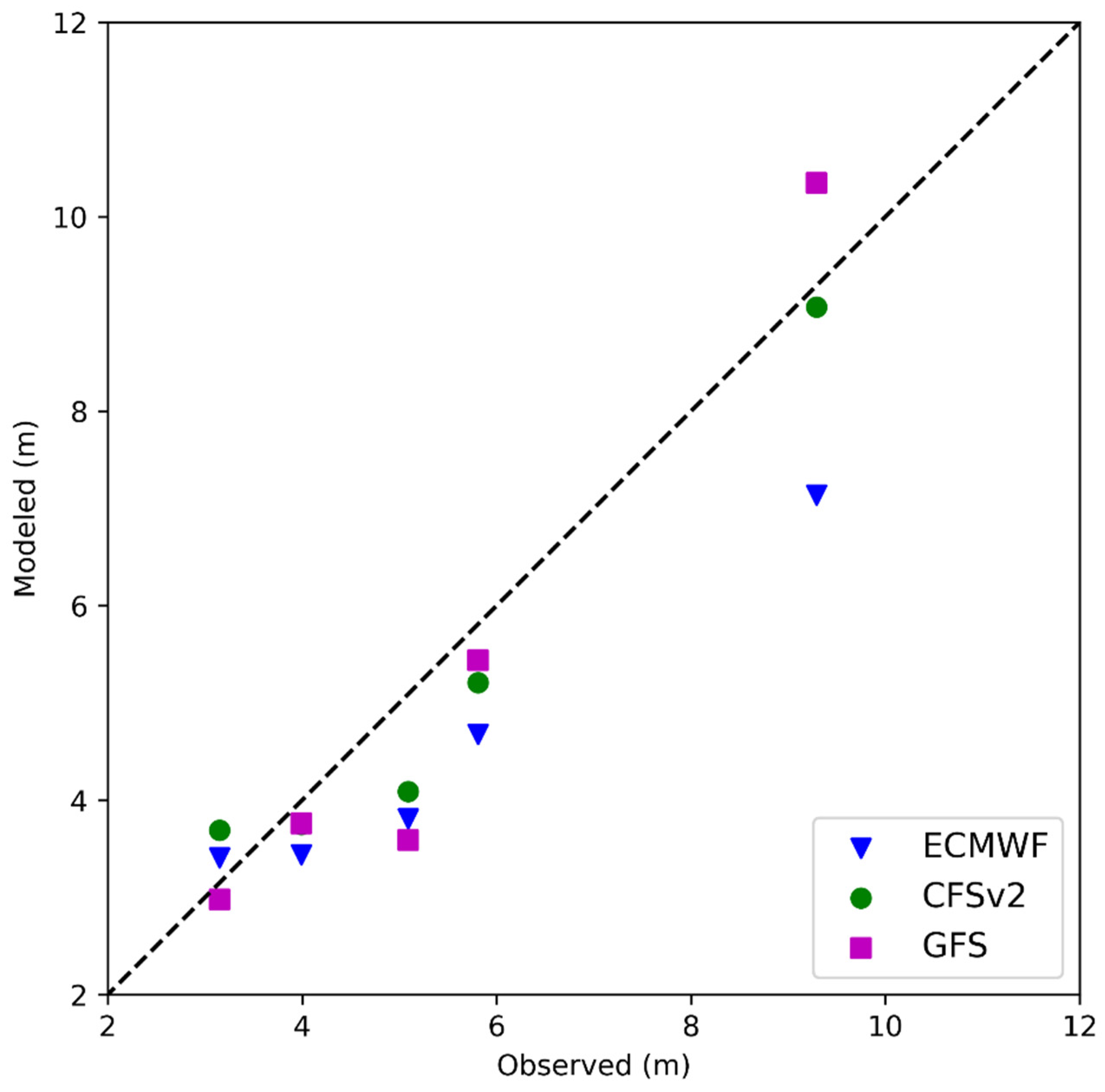
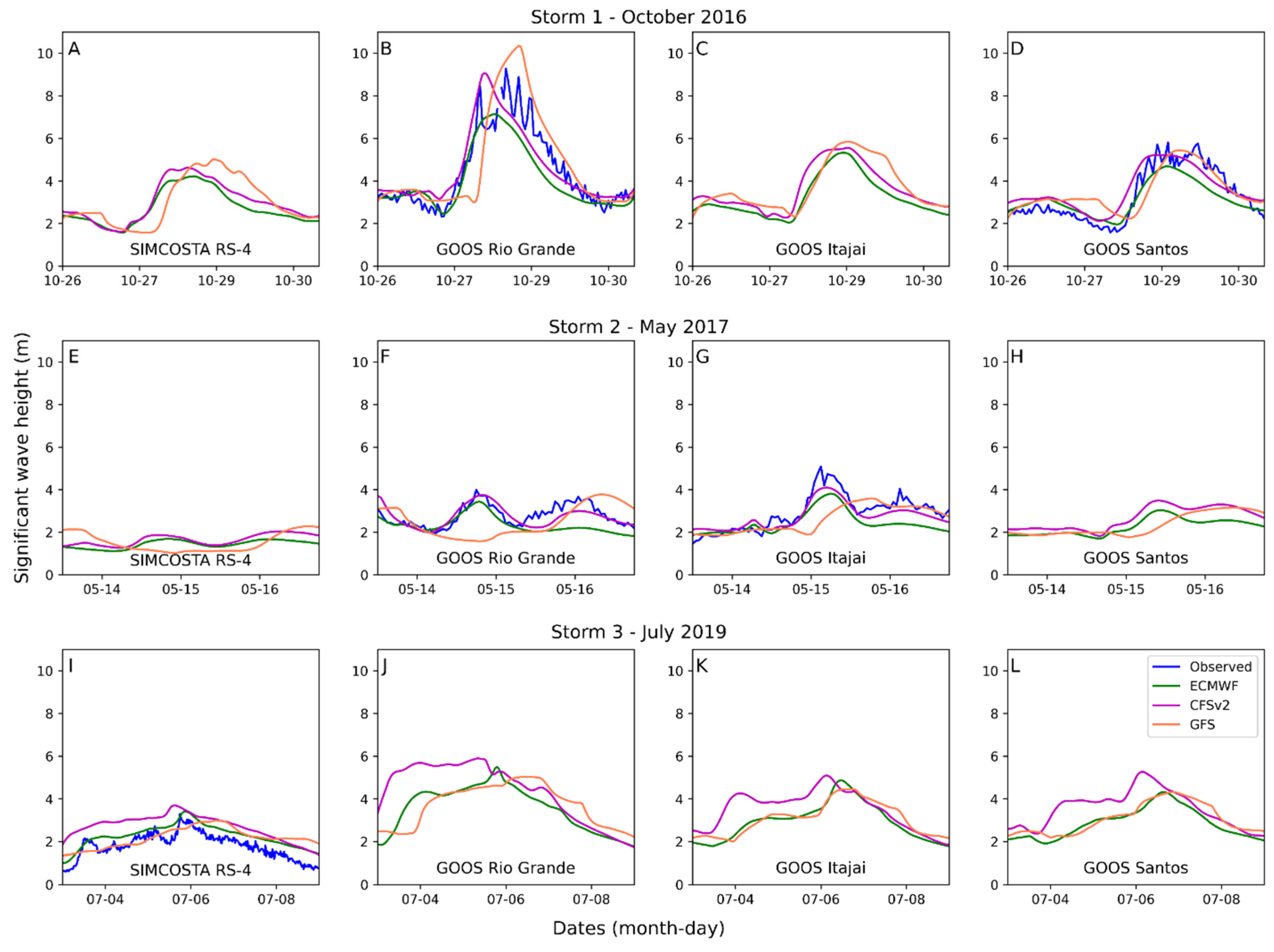
Storm surges can combine the effects of multiple non-linear interactions of oceanic processes (e.g., astronomical tides and wind-generated waves). On the other hand, extreme TWL can also be derived from single intense processes and still cause serious damage to coastal areas [4,5,35]. In this section, the results of our numerical approach and its comparison with observations obtained in three tide gauges located at the Santa Catarina State coastal zone are presented (Figure 1).
Regarding the storm surge peaks, the model was not able to accurately predict the maximum values in all simulations. The modeled TWL peaks were consistently underestimated, as depicted in Figure 9. In Storm 1, the simulation forced by the GFS model presented the best results being capable to reproduce 84% of the maximum observed values. During Storm 2, even the lower water level peaks recorded during a neap tide were substantially underestimated by all sets of simulations. For example, the simulations forced by CFSv2 and GFS presented the best results in Balneario Camboriu station (SC2927); however, with an absolute error of 0.29 and 0.31 m, respectively, there is an almost 40% underestimation. Finally, in Storm 3, the simulation forced by the CFSv2 forced model presented the best results in all three stations. In the Imbituba station (SC2963), the simulation was able to represent 74% of the maximum water levels with an absolute error of 0.28 m. In contrast, a similar research [75] indicated a good agreement between modeled and observed maximum water level values with a relative error up to 2.3%, utilizing the very same modeling approach forced by the CFSv2 model in the South China Sea.
The time series presented in Figure 10 demonstrates that the substantial underestimation observed in the maximum values, in fact, occurs during all selected storm surge events. In Storm 1, despite that the GFS model has provided the best results for maximum values, an overestimation is evident in the subsequential days (Figure 10B,C). Furthermore, the model has presented similar behaviors in Storms 2 and 3, i.e., under normal meteorological conditions the model was able to accurately represent the TWL in all stations, and during the storms, a negligible increase in the water surface elevation is observed. Overall, the model presented a low sensitivity to different meteorological forcing. For instance, in Storm 2, although the CFSv2 completely misrepresented the local pressure fields and the GFS model exhibited a lack of accuracy on the wind magnitudes, the resulting TWL outputs were relatively similar.
Table 1 presents the RMSE for all simulations in terms of TWL and the boldfaced values represent the best results obtained in the set of simulations. Despite that the GFS model has presented a good performance in terms of maximum values, it has been surpassed in all simulations by either ECMWF or CFSv2 models when the entire time series is considered. Additionally, it is important to highlight that the ECMWF model has presented the most consistent RMSE results in all simulations. For instance, while a difference of 1 cm is observed between the ECMWF and the CFSv2 results in Storms 1 and 3 simulation errors, a much larger error in magnitude is observed in Storm 2, where ECMWF is the best meteorological forcing. In addition, Table 2 presents the error metrics for surge only, i.e., disregarding the astronomical tides, which indicates that the error is mostly related to the water piling up caused by the action of meteorological forcing.
Despite that the TWL results pointed out by this research suggest a lack of accuracy in the meteorological forcing, [40] stated that simulations forced by the same climate models led to similarly accurate results for storm surge forecasting in the Northwest Atlantic Ocean, highlighting the ECMWF model efficiency. Moreover, [42], also affirmed that ECMWF stood as a highly accurate climate model, however, with significant spatial dependency in the United States coast. On the other hand, in the Persian Gulf, the GFS model produced the best wind field data and, thus, was more accurate for storm surge numerical modeling applications [41]. Regarding the Southwest Atlantic, our findings are in agreement with [78], which demonstrated that even the most widely used climate models can lead to a fail in up to 50% on TWL hindcasting in our study area.
Lastly, it should be mentioned that the present study does not yet consider the effects of river discharge, rainfall, infragravity waves, wave run-up, as well as depth-dependent processes, such as velocity gradients due to density, that might vary according to different ocean temperature and salinity. According to [80], the South Brazilian Bight (extending from 23° S to 28° S) is highly influenced by the Brazil Current. Moreover, the spatial variability of currents confluence (i.e., Brazil-Malvinas) might as well influence the circulation in the Southern Brazilian Shelf [81]. In a three-dimensional numerical modeling approach, [82] pointed out for the first time that the Brazilian Current has a strong baroclinic impact in the northern portion of the Brazilian Bight.

3.4. Waves

Wind-generated waves may be a significant component of the TWL during a storm event. Moreover, the wave setup might increase coastal flood hazard in wave-tide dominant regions such as the Southern Brazil Bight [83]. According to [4], the dependence of those two elements is dominant in midlatitudes, owing to the fact that the compound effect is generated by the same atmospheric conditions. As stated by [10,47], higher and long-period waves are found in the southern region of the Brazilian coastal zone, along with extreme waves during the winter months. The wave setup that also composes the TWL has a nonnegligible impact in numerical modeling simulations of storm surges, even though in lower magnitude meteorological events its effect might be lower than 10% [75].
The scatterplot presented in Figure 11 depicts a much stronger dependence between observed and modeled wave height maximum values if compared with TWL model results. During the most significant event (Storm 1), the simulation forced by the CFSv2 model was able to represent 98% of the observed peak at the Rio Grande Buoy (Figure 12B). However, at the same validation point, a timing delay between all climate models is observed. As shown in Table 3, despite the models’ accuracy, the maximum value was predicted 10 h ahead of the observed peak, while GFS, which also presented a good performance, was able to force the wave peak with a positive timing shift of 6 h. On the other hand, despite being outperformed by the other climate models, the simulation forced by the ECMWF Era-5 resulted in a wave peak exactly at the same time as the observed at the Santos buoy during the same event. The same situation is even more evident during Storm 3 (Figure 12J) when the same lagging was not observed for the wind forcing products (Figure 8A,H).
Due to a lack of observation data, the evolution of the wave propagation in the study area cannot be completely understood during the selected meteorological events. However, as depicted in Figure 12B,D, a magnitude loss of almost 40% in the wave maximum values is evident after 15 h in a fetch of 816 km. In contrast, in Storm 2, the wave energy evolves in the opposite way, though at a different order of magnitude. In a fetch of 521 km between the Rio Grande and Santos buoys (Figure 12F,G), the wave maximum values show an increase of approximately 20% after 9 h. The authors of [80] stated that the large meteorological variability on the Southwest Atlantic Ocean prevents short-term simulations to fully comprehend the ocean waves’ behavior patterns, suggesting the need for long-term simulations (over 10 years), which cannot be completely validated as a consequence of insufficient wave data. However, a reanalysis based dataset is available as an alternative to describe wave climate along the Brazilian coast [27,84] as well as a long-term-wave database at local scales, e.g., [85].
Overall, the model approach showed good performance for the Hs modeling and a suitable representation with observations is evident. Table 4 shows the Hs error metrics and the boldfaced values represent the best results obtained in the set of simulations. In Storm 1, the simulation forced by CFSv2 presented a better RMSE in both buoys with available observations for the same period, despite that the GFS was a better option in the second buoy for maximum values. The same occurs in Storm 2. The simulation carried out with the CFSv2 forcing resulted in a better RMSE in all available buoys. Even though the GFS model led to a better representation of maximum values, the biggest time-shifting of up to 15 h was observed in both buoys. Finally, in Storm 3, the model results were validated in only one buoy due to the lack of recent observational wave data in Brazil. The RS-4 is the southernmost buoy, as well as the closest to the coast (around 8 km at 32° S). In this case, both the best maximum values and RMSE are related to the ECMWF Era-5 meteorological forcing. Yet, the CFSv2 overpredicted the entire time-series. In a similar investigation, [80] validated the wave heights at the very same set of oceanic buoys in a longer period of simulations, where the RMSE was no lower than 0.46 m in the Rio Grande Buoy and 0.57 m in the Itajai buoy, even though a hybrid oceanic model was employed, using the CFSR climate model. Likewise, [85] presented a similar RMSE order of magnitude (maximum values of 0.58 m for wave heights higher than 1 m) in a local long-term set of simulations validated at 24° S and forced by an ECMWF climate model. On the other hand, in the North Atlantic Ocean, a similar modeling approach applied for wave forecasting showed RMSE values ranging between 0.26 and 0.84 m [86].

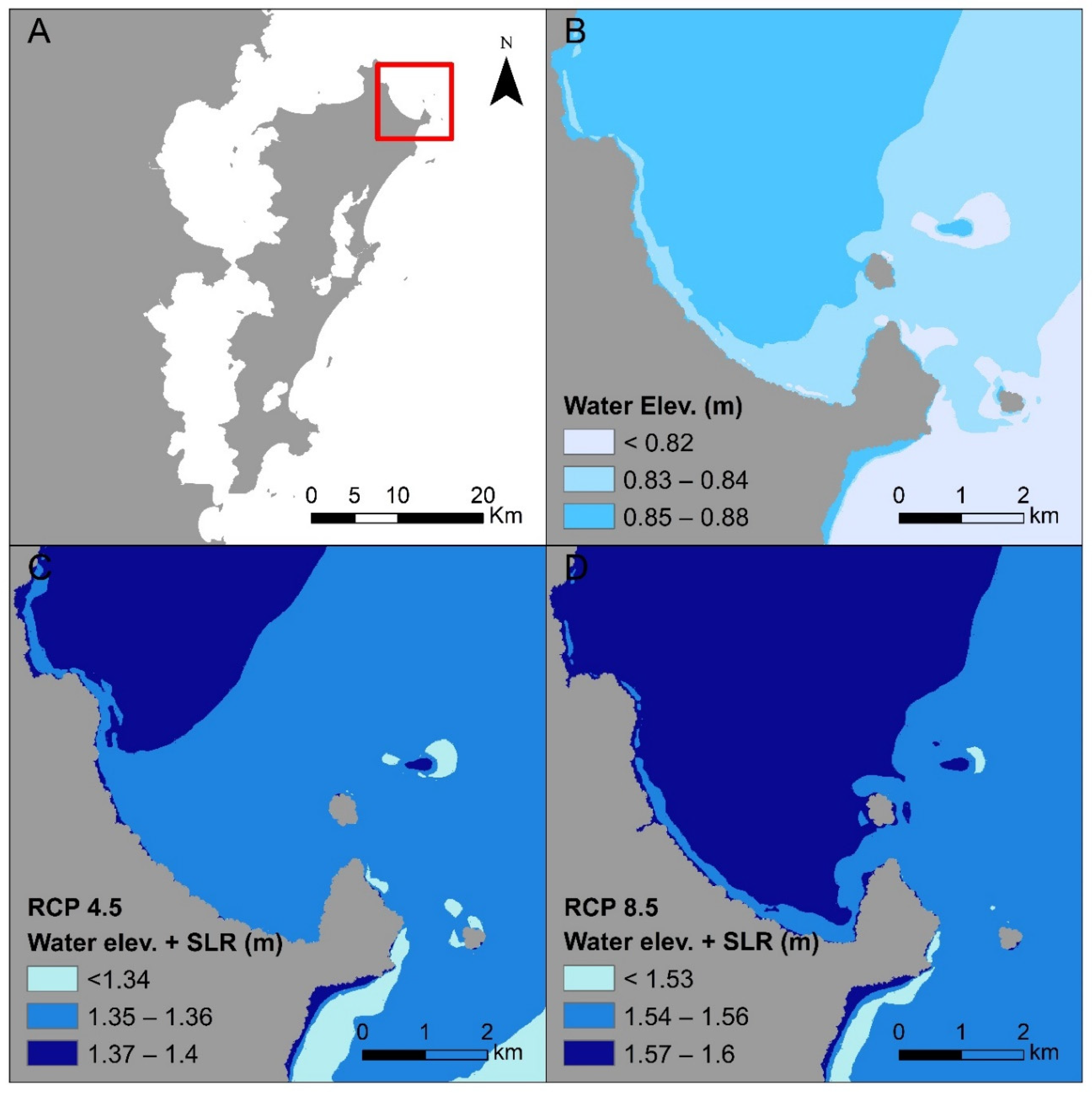
3.5. Local Scale Assessment

The Santa Catarina Island (27.6° S and 48.4° W) is located in the South Region of Brazil and partially composes the territory of Florianopolis, which is the state capital and the second-largest city of the Santa Catarina State (Figure 3C). The island encompasses two different marine domains owing to the fact that it is located at a small distance from the mainland. The Atlantic Ocean domain incorporates both north and east sectors that present reflective and intermediate beaches of different sizes, generally east-southeast-facing, delimited by rocky headlands [87]. In contrast, the west domain, facing a bay system, is sheltered from the direct incidence of waves and is composed of rocky headlands, low energy pocket beaches, and estuarine systems with mangrove occurrence [88]. Florianopolis is the most affected city by storm surges in the state, with an extensive record of both inundation and erosion events, with important repercussions over densely occupied coastal segments and their communities [88,89,90]. The Ingleses beach is a representative case of an area highly susceptible to the effects of storm surges [91,92]. The aforementioned beach is located at the north shore of the island (Figure 13A) and features distinctive characteristics in a retreating coastline [93], where the sheltered areas (southern sector) are densely urbanized and highly susceptible to storm surge impacts, while the semi-exposed areas (northern sector) presents vegetated foredunes that provide, among a large number of local ecosystem services, the coastline protection that locally reduces its susceptibility [92,94].
Figure 13 illustrates three different components of the Storm 1 event describe in this research in a specific and detailed cutoff of our global maximum file outputs, located at the Ingleses beach. The maximum surface elevation over the entire simulation indicates a range between 0.83 and 0.88 m along the beach shore (Figure 13B). Due to its gentle beach face slope [95], the maximum water level values under this storm surge event led to a collision regime even in the northernmost sector, where a wider backshore induces a lower susceptibility to erosion [92]. Moreover, the urbanized shore on the southern sector also registered a collision regime; however, with a direct impact on the urbanized area, where damages had been recorded during this event.
The maximum Hs, as well as the wave direction, are presented in Figure 13C and depict the south-eastern waves being diffracted towards the Ingleses shore. Maximum Hs values of 3.7 m reached the Santa Catarina Island a day after a 5.3 m of Hs was registered at the Itajai buoy on 28 October 2016 (Figure 12C). Nevertheless, on a distinct extreme event, waves with a maximum height of 6.5 m have been recorded adjacent to the Santa Catarina island by [96]. Although the regional wave climate is dominated by south, southeast, and east swells, due to its orientation, the Ingleses beach is protected from south swells, partially sheltered from southeast swells, and mainly exposed to eastern waves [8,95,97]. As a matter of fact, during a southwest event, waves of 1.3 m were hindcasted in the northernmost sector at a 2 m depth, while in the central part of the beach waves of 0.9 m height were obtained and, finally, 0.6 m in the sheltered area in the southernmost beach sector. In a similar analysis, based on a 60-year global reanalysis database, [98] presented the Hs mode values of 0.75 m in both sectors North and Central, while Hs of 0.5 m in the Southern area. The peak wave period (Tp) has shown a significant dependency on the wave direction. Longer peak period waves (14–17 s) were modeled along with all the exposed areas to the incidence of southeastern waves, while in areas where the waves were refracted, such as the Ingleses beach, Tp varies between 6 and 8 s (Figure 13D). This suggests that although the long-period waves from south-southeast are the most frequent in the area, the water level increment observed in this event (also possibly true for the others) appears to be related to waves with shorter periods from northeast-east, generated closer to the shore.
In order to investigate the dependency of the two main storm surge components, i.e., meteorological forcing and astronomical tides, on the TWL, a scenario analysis was conducted in our domain considering two different tidal cycles. The results were also analyzed in the central sector of the Ingleses beach (Figure 14). The astronomical tides along the state of Santa Catarina have a microtidal range, with spring tides varying from 0.46 m in the southernmost area to 1.05 m in the north [87], and according to [88], the Ingleses beach presents a moderate tidal range of 0.6 m. The first scenario (Figure 14A) represents the real event, i.e., the storm surge occurred during a spring tide cycle, when usually coastal flooding and erosion are most likely to happen due to a higher TWL induced by those factors simultaneously. The predicted astronomical tides at the opposite portion of the island indicated a 0.43 m peak, corresponding to 36% of the observed TWL at the tide gauge. On the other hand, at Ingleses beach, a 0.43 m peak was predicted in our simulation. In contrast, while a TWL of 1.21 m was observed at the Florianopolis tide gauge, a 0.82 TWL peak was simulated independently of different meteorological forcing. Finally, Figure 14B shows the second scenario, which demonstrates both TWL and tides for the same meteorological forcing under a neap tide cycle. In this scenario, a 0.23 m tide peak was predicted and a 0.54 m TWL peak was simulated, indicating that under different astronomical conditions, Storm 1 could have reached a peak of at least 0.2 m lower.
As a second analysis, two different 2100 SLR scenarios were implemented as fixed mean sea level offsets of 0.53 and 0.74 m, according to the IPCC RCPs 4.5 and 8.5, respectively [14]. Several physical impacts are expected globally due to SLR in the 21st century, such as an increase in flooding events and the submergence of low-elevation coastal zones. Moreover, longer-term effects related to the coastal adjustment to new morphodynamic conditions can lead to severe erosion and the compromise of coastal aquifers due to saline intrusion [99]. These impacts, therefore, will exacerbate socio-economic damage in more vulnerable coastal communities. For instance, in the Brazilian southeast region, the SLR is expected to produce a significant impact on the Santos Estuarine system in 2100, when almost 50% of its mangroves will be flooded as well as part of the adjacent beaches [100]. Although the SLR effects have been globally studied, on a local scale those impacts are under-reported in Brazil, thus making it difficult to be considered in coastal management, such as in the case of Florianopolis. However, a coastal sensitivity and population exposure to SLR assessment presented by [88] pointed out that Ingleses beach presents a high population exposure to SLR in its southern sector, even though it has a sheltered characteristic. On the other hand, in areas with a low population density such as the northern sector, the exposure is, naturally, lower even with a high susceptibility to erosion.
Figure 15 shows the SLR scenario analysis conducted at the Ingleses beach considering the most significant among the analyzed storm events (Storm 1), of which the magnitude has not undergone any changes as well as the original tidal cycle. Therefore, Figure 15B represents the original storm surge amplitude at the TWL peak while Figure 15C,D show the predicted offsets added in order to simulate the IPCC RCPs 4.5 and 8.5, respectively. In the first scenario, the maximum accumulated value referring to the original TWL and the SLR offset represents an increase of approximately 60% in the water surface elevation. Furthermore, the second scenario suggests an even more significant change in the storm surge effects, indicating an increase of approximately 82% over the original TWL. Although the model does not present an approach that quantifies coastal erosion, it is worthwhile to mention that such a significant change in the TWL might potentially impact the entire surf zone, leading to a local morphodynamic readjustment and, therefore, altering the entire beach profile.
The SLR effects will also impact regular oceanographic conditions. In southern Brazil, storm surges occur every 6.5 to 11 days [9], and regardless of their magnitude, a collision regime at Ingleses beach may occur during spring tides. In this context, the frontal dunes in the northern sector of the beach have the potential to be even more essential in providing coastal protection and stabilization. This ecosystem has only a remnant of frontal dunes, extending for only 20% of the beach.

4. Conclusions

The coupled ADCIRC+SWAN hydrodynamic and phase-average wave numerical modeling framework was presented as an alternative for storm surge hindcasting and SLR scenario analysis on the Southern Brazilian coast given the significant data scarcity constraints of the region. Moreover, the models’ dependency on different sources of meteorological forcing was investigated considering three different wind and pressure field sources i.e., the Fifth Generation of ECMWF Atmospheric Reanalysis (ERA 5), Climate Forecast System Version 2 (CFSv2), and the Global Forecast System (GFS). The results demonstrate that with regards to astronomical tides, the modeling approach presented a good agreement with the tide gauge predictions in terms of amplitudes. Concerning the meteorological events simulations, although constantly underestimating TWL values, the Hs results presented good accordance with observational data, despite the evident inaccuracy of the wind magnitude data. The results showed significantly low sensitivity to different meteorological forcing; however, the CFSv2 model stood out as the most consistent meteorological forcing for storm surge and waves numerical hindcast, and ERA5 was highlighted as the second most accurate meteorological forcing while adequately simulating the peak timings. The lower predictability of the GFS meteorological forcing could be attributed to its coarser resolution.
Furthermore, three scenario analyzes were conducted in order to demonstrate different model applications on a local scale. First, the astronomical tide amplitudes influence on the TWL was investigated during a storm surge event. It was demonstrated that in a specific event, the co-occurrence of the storm that arises during a spring tide had an impact of 20% on the TWL. Although governed by a microtidal regime, the astronomical tides stood out as a significant storm surge component in the study area. Furthermore, a correct prediction of astronomical tides represents paramount importance when implementing the modeling approach as a framework for forecasting hydrodynamic and wave conditions. Second, two different 2100 SLR scenarios were implemented in accordance with the IPCC RCPs 4.5 and 8.5. In the first scenario, a possible increase of up to 60% was determined in the TWL during Storm 1, inducing higher water levels along the beach, while in the second scenario an 82% increase was predicted. The proposed framework is an invaluable asset to support the Brazilian Plan to Climate Change Adaptation at Coastal Zones, as it is considered that SLR will cause coastal erosion and flooding, saline intrusion, and impacts on natural resources and biodiversity.
Despite the limitations imposed by the lack of continuous and densely distributed observational data, as well as up to date topobathymetric datasets, the proposed framework is capable of expanding TWL and Hs information, previously only available to a handful of gauge stations, to a spatially distributed and temporally unlimited scale. This more comprehensive understanding of such extreme events represents valuable knowledge for the potential implementation of more adequate coastal management and engineering practices for the Brazilian coastal zone, especially under changing climate conditions. Furthermore, the proposed methodology can highly contribute to the Brazilian Program for Shoreline Conservation (ProCosta), a shoreline management initiative that aggregates projects dealing with updating topobathymetric datasets; projection of future coastlines and hazard identification; and coastal risk and adaptation strategies. In addition, as a recommendation for future research, the influence of both the Malvinas and Brazil currents can be incorporated into the model domain in order to understand the regional oceanic circulation effects in the storm surge propagation.

Supplementary Materials

The following are available online at https://www.mdpi.com/2073-4441/12/12/3538/s1, Figure S1: Harmonic Constituent Phases for three different stations in the Santa Catarina State coastal areas.

Author Contributions

Conceptualization, A.d.S.d.L., C.F., M.E.G.S., and J.B.; Formal analysis, A.d.S.d.L. and A.K.; Funding acquisition, A.d.S.d.L.; Investigation, A.d.S.d.L., A.K., T.W.M., F.C., C.F., M.E.G.S., and J.B.; Methodology, A.d.S.d.L., A.K., T.W.M., and F.C.; Project administration, A.d.S.d.L.; Supervision, C.F., M.E.G.S., and J.B.; Validation, A.d.S.d.L.; Visualization, T.W.M., F.C., and M.E.G.S.; Writing—original draft, A.d.S.d.L.; Writing—review and editing, A.K., T.W.M., F.C., C.F., and J.B. All authors have read and agreed to the published version of the manuscript.

Funding

This study was financed in part by the Coordenação de Aperfeiçoamento de Pessoal de Nível Superior—Brasil (CAPES)—Finance Code 001, CNPq (Grant 306633/2019-1) and the Programa de Pós-Graduação em Geografia, Federal University of Santa Catarina.

Acknowledgments

The authors acknowledge the Santa Catarina Environmental Resources and Hydrometeorology Information Center—Epagri/CIRAM by providing oceanographic observational data for model validation. This work utilized the Extreme Science and Engineering Discovery Environment (XSEDE) STAMPEDE2 resources through allocation id TG-BCS130009, which is supported by the National Science Foundation [grant number ACI- 1548562].

Conflicts of Interest

The authors declare no conflict of interest.

References

  1. Yin, K.; Xu, S.; Zhao, Q.; Huang, W.; Yang, K.; Guo, M. Effects of land cover change on atmospheric and storm surge modeling during typhoon event. Ocean Eng. 2020, 199, 106971. [Google Scholar] [CrossRef]
  2. Alexander, K.S.; Ryan, A.; Measham, T.G. Managed retreat of coastal communities: Understanding responses to projected sea level rise. J. Environ. Plan. Manag. 2012, 55, 409–433. [Google Scholar] [CrossRef]
  3. Staneva, J.; Wahle, K.; Koch, W.; Behrens, A.; Fenoglio-Marc, L.; Stanev, E.V. Coastal flooding: Impact of waves on storm surge during extremes—A case study for the German Bight. Nat. Hazards Earth Syst. Sci. 2016, 16, 2373–2389. [Google Scholar] [CrossRef] [Green Version]
  4. Marcos, M.; Rohmer, J.; Vousdoukas, M.I.; Mentaschi, L.; Le Cozannet, G.; Amores, A. Increased Extreme Coastal Water Levels Due to the Combined Action of Storm Surges and Wind Waves. Geophys. Res. Lett. 2019, 46, 4356–4364. [Google Scholar] [CrossRef] [Green Version]
  5. Lopes, C.L.; Dias, J.M. Assessment of flood hazard during extreme sea levels in a tidally dominated lagoon. Nat. Hazards 2015, 77, 1345–1364. [Google Scholar] [CrossRef]
  6. Lyddon, C.; Brown, J.M.; Leonardi, N.; Plater, A.J. Flood Hazard Assessment for a Hyper-Tidal Estuary as a Function of Tide-Surge-Morphology Interaction. Estuaries Coasts 2018, 41, 1565–1586. [Google Scholar] [CrossRef] [Green Version]
  7. Batstone, C.; Lawless, M.; Tawn, J.; Horsburgh, K.; Blackman, D.; McMillan, A.; Worth, D.; Laeger, S.; Hunt, T. A UK best-practice approach for extreme sea-level analysis along complex topographic coastlines. Ocean Eng. 2013, 71, 28–39. [Google Scholar] [CrossRef]
  8. Muler, M.; Bonetti, J. An Integrated Approach to Assess Wave Exposure in Coastal Areas for Vulnerability Analysis. Mar. Geod. 2014, 37, 220–237. [Google Scholar] [CrossRef]
  9. Ohz, A.; Klein, A.H.F.; Franco, D. A Multiple Linear Regression-Based Approach for Storm Surge Prediction Along South Brazil. In Climate Change, Hazards and Adaptation Options; Springer International Publishing: Cham, Switzerland, 2020; pp. 369–388. ISBN 978-3-030-37424-2. [Google Scholar]
  10. Rodríguez, M.G.; Nicolodi, J.L.; Gutiérrez, O.Q.; Losada, V.C.; Hermosa, A.E. Brazilian Coastal Processes: Wind, Wave Climate and Sea Level. In Brazilian Beach Systems; Short, A.D., Klein, A.H.d.F., Eds.; Springer International Publishing: Cham, Switzerland, 2016; pp. 37–66. ISBN 978-3-319-30392-5. [Google Scholar]
  11. CEPED. Relatório dos Danos materiais e Prejuízos Decorrentes de Desastres Naturais em Santa Catarina: 1995–2014; Schadeck, R., Ed.; Centro Universitário de Estudos e Pesquisas sobre Desastres: Florianópolis, Brazil, 2016.
  12. McTaggart-Cowan, R.; Bosart, L.F.; Davis, C.A.; Atallah, E.H.; Gyakum, J.R.; Emanuel, K.A. Analysis of Hurricane Catarina (2004). Am. Meteorol. Soc. 2006, 134, 3029–3053. [Google Scholar] [CrossRef]
  13. Marcelino, E.V. Impact of the Catarina cyclone on the southern region of Santa Catarina: Field observations. Rev. Def. Civ. 2005, 1, 4–8. [Google Scholar]
  14. Church, J.A.; Clark, P.U.; Cazenave, A.; Gregory, J.M.; Jevrejeva, S.; Levermann, A.; Merrifield, M.A.G.A.; Milne, R.S.; Nerem, P.D.N.; Payne, A.J.; et al. Sea Level Change. In Climate Change 2013: The Physical Science Basis. Contribution of Working Group I to the Fifth Assessment Report of the Intergovernmental Panel on Climate Change; Stocker, T.F.D., Qin, G.-K.P.M., Tignor, S.K.A., Boschung, J., Nauels, A.Y., Xia, V.B., Midgley, P.M., Eds.; Cambridge University Press: Cambridge, UK, 2013. [Google Scholar]
  15. Liu, S.K. Using coastal models to estimate effects of sea level rise. Ocean Coast. Manag. 1997, 37, 85–94. [Google Scholar] [CrossRef]
  16. Mcleod, E.; Poulter, B.; Hinkel, J.; Reyes, E.; Salm, R. Sea-level rise impact models and environmental conservation: A review of models and their applications. Ocean Coast. Manag. 2010, 53, 507–517. [Google Scholar] [CrossRef]
  17. Esteban, M.; Takagi, H.; Jamero, L.; Chadwick, C.; Erick, J.; Mikami, T.; Fatma, D.; Yamamoto, L.; Danh, N.; Onuki, M.; et al. Adaptation to sea level rise: Learning from present examples of land subsidence. Ocean Coast. Manag. 2020, 189, 104852. [Google Scholar] [CrossRef]
  18. Abadie, L.M.; Jackson, L.P.; Sainz, E.; Murieta, D.; Jevrejeva, S. Comparing urban coastal flood risk in 136 cities under two alternative sea-level projections: RCP 8.5 and an expert opinion-based high-end scenario. Ocean Coast. Manag. 2020, 193, 105249. [Google Scholar] [CrossRef]
  19. Irish, J.L.; Frey, A.E.; Rosati, J.D.; Olivera, F.; Dunkin, L.M.; Kaihatu, J.M.; Ferreira, C.M.; Edge, B.L. Potential implications of global warming and barrier island degradation on future hurricane inundation, property damages, and population impacted. Ocean Coast. Manag. 2010, 53, 645–657. [Google Scholar] [CrossRef]
  20. Konisky, D.M.; Hughes, L.; Kaylor, C.H. Extreme weather events and climate change concern. Clim. Chang. 2016, 134, 533–547. [Google Scholar] [CrossRef]
  21. Woth, K.; Weisse, R.; Von Storch, H. Climate change and North Sea storm surge extremes: An ensemble study of storm surge extremes expected in a changed climate projected by four different regional climate models. Ocean Dyn. 2006, 56, 3–15. [Google Scholar] [CrossRef]
  22. Li, R.; Xie, L.; Liu, B.; Guan, C. On the sensitivity of hurricane storm surge simulation to domain size. Ocean Model. 2013, 67, 1–12. [Google Scholar] [CrossRef]
  23. Liu, H.; Zhang, K.; Li, Y.; Xie, L. Numerical study of the sensitivity of mangroves in reducing storm surge and flooding to hurricane characteristics in southern Florida. Cont. Shelf Res. 2013, 64, 51–65. [Google Scholar] [CrossRef]
  24. Harari, J. Desenvolvimento de um modelo numérico hidrodinâmico tri-dimensaional linear, para a simulação e a previsão da circulação na plataforma brasileira entre 23 e 26S. Bol. Inst. Ocean. 1985, 33, 159–191. [Google Scholar] [CrossRef] [Green Version]
  25. Cirano, M.; Campos, E.J.D. Numerical diagnostic of the circulation in the Santos Bight with COROAS hydrographic data. Rev. Bras. Oceanogr. 1996, 44, 105–121. [Google Scholar] [CrossRef] [Green Version]
  26. Harari, J.; De Camargo, R. Numerical simulation of the tidal propagation in the coastal region of Santos (Brazil, 24° S 46° W). Cont. Shelf Res. 2003, 23, 1597–1613. [Google Scholar] [CrossRef]
  27. Quetzalcóatl, O.; González, M.; Cánovas, V.; Medina, R.; Espejo, A.; Klein, A.; Tessler, M.G.; Almeida, L.R.; Jaramillo, C.; Garnier, R.; et al. SMCε, a coastal modeling system for assessing beach processes and coastal interventions: Application to the Brazilian coast. Environ. Model. Softw. 2019, 116, 131–152. [Google Scholar] [CrossRef]
  28. Candella, R.N.; Souza, S.M.L. Ondas oceânicas extremas na costa sul-sudeste Brasileira geradas por ciclone com trajetória anormal em maio de 2011. Rev. Bras. Meteorol. 2013, 28, 441–456. [Google Scholar] [CrossRef] [Green Version]
  29. Pezzi, L.P.; Souza, R.B. De A Review on the Ocean-Atmosphere Interaction Processes in Regions of Strong Sea Surface Temperature Gradients of The South Atlantic Ocean Based on Observational Data. Rev. Bras. Meteorol. 2016, 31, 428–453. [Google Scholar] [CrossRef] [Green Version]
  30. Parodi, M.U.; Giardino, A.; Dongeren, A.; Van Pearson, S.G.; Bricker, J.D.; Reniers, J.H.M. Uncertainties in Coastal Flood Risk Assessments in Small Island Developing States. Nat. Hazards Earth Syst. Sci. 2020, 20, 2397–2414. [Google Scholar] [CrossRef]
  31. van Berchum, E.; van Ledden, M.; Timmermans, J.; Kwakkel, J.; Jonkman, S. Rapid flood risk screening model for compound flood events in Beira, Mozambique. Nat. Hazards Earth Syst. Sci. 2020, 10, 2633–2646. [Google Scholar] [CrossRef]
  32. Mimura, N. Vulnerability of island countries in the South Pacific to sea level rise and climate change. Clim. Res. 1999, 12, 137–143. [Google Scholar] [CrossRef]
  33. Dietrich, J.C.; Zijlema, M.; Westerink, J.J.; Holthuijsen, L.H.; Dawson, C.; Luettich, R.A.; Jensen, R.E.; Smith, J.M.; Stelling, G.S.; Stone, G.W. Modeling hurricane waves and storm surge using integrally-coupled, scalable computations. Coast. Eng. 2011, 58, 45–65. [Google Scholar] [CrossRef]
  34. Deb, M.; Ferreira, C.M. Simulation of cyclone-induced storm surges in the low-lying delta of Bangladesh using coupled hydrodynamic and wave model (SWAN + ADCIRC). J. Flood Risk Manag. 2018, 11, S750–S765. [Google Scholar] [CrossRef]
  35. Murty, P.L.N.; Bhaskaran, P.K.; Gayathri, R.; Sahoo, B.; Kumar, T.S.; SubbaReddy, B. Numerical study of coastal hydrodynamics using a coupled model for Hudhud cyclone in the Bay of Bengal. Estuar. Coast. Shelf Sci. 2016, 183, 13–27. [Google Scholar] [CrossRef]
  36. Moradi, M.; Kazeminezhad, M.H.; Kabiri, K. Integration of Geographic Information System and system dynamics for assessment of the impacts of storm damage on coastal communities-Case study: Chabahar, Iran. Int. J. Disaster Risk Reduct. 2020, 49, 101665. [Google Scholar] [CrossRef]
  37. Cyriac, R.; Dietrich, J.C.; Fleming, J.G.; Blanton, B.O.; Kaiser, C.; Dawson, C.N.; Luettich, R.A. Variability in Coastal Flooding predictions due to forecast errors during Hurricane Arthur. Coast. Eng. 2018, 137, 59–78. [Google Scholar] [CrossRef]
  38. Dube, S.K.; Murty, T.S.; Feyen, J.C.; Cabrera, R.; Harper, B.A.; Bales, J.D.; Amer, S. Storm Surge Modeling and Applications in Coastal Areas. In Global Perspectives on Tropical Cyclones; Chan, J.C.L., Kepert, J.D., Eds.; World Scientific: River Edge, NJ, USA, 2010; pp. 363–406. ISBN 978-981-4293-48-8. [Google Scholar]
  39. Mauritzen, C.; Zivkovic, T.; Veldore, V. On the relationship between climate sensitivity and modelling uncertainty. Tellus Ser. Dyn. Meteorol. Oceanogr. 2017, 69, 1–12. [Google Scholar] [CrossRef] [Green Version]
  40. Garzon, J.L.; Ferreira, C.M.; Padilla-Hernandez, R. Evaluation of weather forecast systems for storm surge modeling in the Chesapeake Bay. Ocean Dyn. 2018, 68, 91–107. [Google Scholar] [CrossRef]
  41. Afshar-Kaveh, N.; Ghaheri, A.; Chegini, V.; Etemad-Shahidi, A.; Nazarali, M. Evaluation of Different Wind Fields for Storm Surge Modeling in the Persian Gulf. J. Coast. Res. 2016, 33, 596–606. [Google Scholar] [CrossRef] [Green Version]
  42. Wedam, G.B.; McMurdie, L.A.; Mass, C.F. Comparison of model forecast skill of sea level pressure along the east and west coasts of the United States. Weather Forecast. 2009, 24, 843–854. [Google Scholar] [CrossRef] [Green Version]
  43. Vieira, G.B.B.; Neto, F.J.K.; Ribeiro, J.L.D. The Rationalization of Port Logistics Activities: A Study at Port of Santos (Brazil). Int. J. e-Navig. Marit. Econ. 2015, 2, 73–86. [Google Scholar] [CrossRef] [Green Version]
  44. Diegues, A.C. Human populations and coastal wetlands: Conservation and management in Brazil. Ocean Coast. Manag. 1999, 42, 187–210. [Google Scholar] [CrossRef]
  45. Matano, R.P.; Palma, E.D.; Piola, A.R. The influence of the Brazil and Malvinas Currents on the Southwestern Atlantic Shelf circulation. Ocean Sci. 2010, 6, 983–995. [Google Scholar] [CrossRef] [Green Version]
  46. Cuchiara, D.C.; Fernandes, E.H.; Strauch, J.C.; Winterwerp, J.C.; Calliari, L.J. Determination of the wave climate for the southern Brazilian shelf. Cont. Shelf Res. 2009, 29, 545–555. [Google Scholar] [CrossRef]
  47. Araujo, C.E.S.; Franco, D.; Melo, E.; Pimenta, F. Wave regime characteristics of the southern Brazilian coast. In Proceedings of the Sixth International Conference on Coastal and Port Engineering in Developing Countries, Colombo, Sri Lanka, 15–19 September 2003. [Google Scholar]
  48. Gan, M.A.; Rao, V.B. Surface Cyclogenesis over South America. Am. Meteorol. Soc. 1991, 119, 1293–1302. [Google Scholar] [CrossRef]
  49. Gramcianinov, C.B.; Hodges, K.I.; Camargo, R. The properties and genesis environments of South Atlantic cyclones. Clim. Dyn. 2019, 53, 4115–4140. [Google Scholar] [CrossRef]
  50. Saraiva, J.M.B.; Bedran, C.; Carneiro, C.; Saraivaf, J.M.B.; Bedranf, C.; Carneiro, C. Monitoring of Storm Surges on Cassino Beach, RS, Brazil. J. Coast. Res. 2003, 323–331. [Google Scholar]
  51. Machado, A.A.; Calliari, L.J. Synoptic Systems Generators of Extreme Wind in Southern Brazil: Atmospheric Conditions and Consequences in the Coastal Zone. J. Coast. Res. 2016, 75, 1182–1186. [Google Scholar] [CrossRef]
  52. Serafim, M.B.; Siegle, E.; Corsi, A.C.; Bonetti, J. Coastal vulnerability to wave impacts using a multi-criteria index: Santa Catarina (Brazil). J. Environ. Manag. 2019, 230, 21–32. [Google Scholar] [CrossRef]
  53. Dube, S.K.; Jain, I.; Rao, A.D.; Murty, T.S. Storm surge modelling for the Bay of Bengal and Arabian Sea. Nat. Hazards 2009, 51, 3–27. [Google Scholar] [CrossRef]
  54. Sebastian, A.; Proft, J.; Dietrich, J.C.; Du, W.; Bedient, P.B.; Dawson, C.N. Characterizing hurricane storm surge behavior in Galveston Bay using the SWAN + ADCIRC model. Coast. Eng. 2014, 88, 171–181. [Google Scholar] [CrossRef]
  55. Wang, Y.; Mao, X.; Jiang, W. Long-term hazard analysis of destructive storm surges using the ADCIRC-SWAN model: A case study of Bohai Sea, China. Int. J. Appl. Earth Obs. Geoinf. 2018, 73, 52–62. [Google Scholar] [CrossRef]
  56. Lawler, S.; Haddad, J.; Ferreira, C.M. Sensitivity considerations and the impact of spatial scaling for storm surge modeling in wetlands of the Mid-Atlantic region. Ocean Coast. Manag. 2016, 134, 226–238. [Google Scholar] [CrossRef] [Green Version]
  57. Luettich, R.A.; Westerink, J.J.; Scheffner, N.W. ADCIRC: An Advanced Three-Dimensional Circulation Model for Shelves Coasts and Estuaries, Report 1: Theory and Methodology of ADCIRC-2DDI and ADCIRC-3DL, Dredging Research Program Technical Report DRP-92-6; US Army Corps of Engineers: Washington, DC, USA, 1992. [Google Scholar]
  58. Ferreira, C.M.; Olivera, F.; Irish, J.L. Arc StormSurge: Integrating Hurricane Storm Surge Modeling and GIS. JAWRA J. Am. Water Resour. Assoc. 2014, 50, 219–233. [Google Scholar] [CrossRef]
  59. Garzon, J.L.; Ferreira, C.M. Storm surge modeling in large estuaries: Sensitivity analyses to parameters and physical processes in the Chesapeake Bay. J. Mar. Sci. Eng. 2016, 4, 45. [Google Scholar] [CrossRef] [Green Version]
  60. Xie, D.M.; Zou, Q.P.; Cannon, J.W. Application of SWAN+ADCIRC to tide-surge and wave simulation in Gulf of Maine during Patriot’s Day storm. Water Sci. Eng. 2016, 9, 33–41. [Google Scholar] [CrossRef] [Green Version]
  61. Booij, N.; Ris, R.C.; Holthuijsen, L.H. A third-generation wave model for coastal regions. J. Geophical Res. 1999, 104, 7649–7666. [Google Scholar] [CrossRef] [Green Version]
  62. Kalyanapu, A.J.; Burian, S.J.; McPherson, T.N. Effect of land use-based surface roughness on hydrologic model output. J. Spat. Hydrol. 2009, 9, 51–71. [Google Scholar]
  63. Mussi, C.S. Mapeamento da Geodiversidade e Análise de Bens e Serviços Ecossistêmicos Prestados Pela Plataforma Continental de Santa Catarina, Brasil. Master’s Dissertation, Santa Catarina Federal University, Florianópolis, Brazil, 2017; p. 204, Unpublished work. [Google Scholar]
  64. Madsen, O.S.; Poon, Y.-K.; Graber, H.C. Spectral wave attenuation by bottom friction: Theory. In Proceedings of the 21st International Conference on Coastal Engineering, Malaga, Spain, 20–25 June 1988; American Society of Civil Engineers: Malaga, Spain, 1988; pp. 492–504. [Google Scholar]
  65. Roberts, K.J.; Pringle, W.J.; Westerink, J.J. OceanMesh2D 1.0: MATLAB-based software for two-dimensional unstructured mesh generation in coastal ocean modeling. Geosci. Model Dev. 2019, 12, 1847–1868. [Google Scholar] [CrossRef] [Green Version]
  66. GEBCO. Compilation Group General Bathymetric Chart of the Oceans; British Oceanographic Data Centre: Liverpool, UK, 2019. [Google Scholar]
  67. Secretaria de Estado do Desenvolvimento Economico Sustentavel—SDS. Levantamento Aerofotogramétrico 2010-Modelo Digital de Terreno; Secretaria de Estado do Desenvolvimento Economico Sustentavel: Santa Catarina, Brazil, 2010.
  68. Wessel, P.; Smith, W.H.F. A global, self-consistent, hierarchical, high-resolution shoreline database. J. Geophys. Res. Solid Earth 1996, 101, 8741–8743. [Google Scholar] [CrossRef] [Green Version]
  69. Hersbach, H.; Bell, B.; Berrisford, P.; Hirahara, S.; Horányi, A.; Nicolas, J.; Peubey, C.; Radu, R.; Bonavita, M.; Dee, D.; et al. The ERA5 Global Reanalysis. Q. J. R. Meteorol. Soc. 2020, 1–51. [Google Scholar] [CrossRef]
  70. Yang, F.; Pan, H.L.; Krueger, S.K.; Moorthi, S.; Lord, S.J. Evaluation of the NCEP global forecast system at the ARM SGP site. Mon. Weather Rev. 2006, 134, 3668–3690. [Google Scholar] [CrossRef]
  71. Saha, S.; Moorthi, S.; Wu, X.; Wang, J.; Nadiga, S.; Tripp, P.; Behringer, D.; Hou, Y.T.; Chuang, H.Y.; Iredell, M.; et al. The NCEP climate forecast system version 2. J. Clim. 2014, 27, 2185–2208. [Google Scholar] [CrossRef]
  72. Egbert, G.D.; Erofeeva, S.Y. Efficient Inverse Modeling of Barotropic Ocean Tides. J. Atmos. Ocean. Technol. 2002, 19, 183–204. [Google Scholar] [CrossRef] [Green Version]
  73. Joyce, B.R.; Pringle, W.J.; Wirasaet, D.; Westerink, J.J.; Van der Westhuysen, A.J.; Grumbine, R.; Feyen, J. High resolution modeling of western Alaskan tides and storm surge under varying sea ice conditions. Ocean Model. 2019, 141, 101421. [Google Scholar] [CrossRef]
  74. Defant, A. Physical Oceanography, 2nd ed.; Pergamon: New York, NY, USA, 1961. [Google Scholar]
  75. Li, A.; Guan, S.; Mo, D.; Hou, Y.; Hong, X.; Liu, Z. Modeling wave effects on storm surge from different typhoon intensities and sizes in the South China Sea. Estuar. Coast. Shelf Sci. 2020, 235, 106551. [Google Scholar] [CrossRef]
  76. Chai, T.; Oceanic, N. Root Mean Square Error (RMSE) or Mean Absolute Error (MAE)?–Arguments against Avoiding RMSE in the Literature. Geosci. Model Dev. 2015, 7, 1247–1250. [Google Scholar] [CrossRef] [Green Version]
  77. Franz, G.A.S.; Leitão, P.; dos Santos, A.; Juliano, M.; Neves, R. From regional to local scale modelling on the south-eastern Brazilian shelf: Case study of Paranaguá estuarine system. Braz. J. Oceanogr. 2016, 64, 277–294. [Google Scholar] [CrossRef] [Green Version]
  78. Dinápoli, M.G.; Simionato, C.G.; Moreira, D. Nonlinear tide-surge interactions in the Río de la Plata Estuary. Estuar. Coast. Shelf Sci. 2020, 241, 106834. [Google Scholar] [CrossRef]
  79. WMO. Guide to Storm Surge Forecasting; World Meteorological Organization: Geneva, Switzerland, 2011; ISBN 978-92-63-11076-3. [Google Scholar]
  80. Kirinus, E.d.P.; Oleinik, P.H.; Costi, J.; Marques, W.C. Long-term simulations for ocean energy off the Brazilian coast. Energy 2018, 163, 364–382. [Google Scholar] [CrossRef]
  81. Palma, E.D.; Matano, R.P.; Piola, A.R. A numerical study of the Southwestern Atlantic Shelf circulation: Barotropic response to tidal and wind forcing. J. Geophys. Res. Ocean. 2004, 109, 1–17. [Google Scholar] [CrossRef]
  82. Pereira, A.F.; Castro, B.M.; Calado, L.; da Silveira, I.C.A. Numerical simulation of M2 internal tides in the South Brazil Bight and their interaction with the Brazil Current. J. Geophys. Res. Ocean. 2007, 112. [Google Scholar] [CrossRef] [Green Version]
  83. Rueda, A.; Vitousek, S.; Camus, P.; Tomás, A.; Espejo, A.; Losada, I.J.; Barnard, P.L.; Erikson, L.H.; Ruggiero, P.; Reguero, B.G.; et al. A global classification of coastal flood hazard climates associated with large-scale oceanographic forcing. Sci. Rep. 2017, 7, 5038. [Google Scholar] [CrossRef]
  84. Silva, P.G.; Klein, A.H.F.; González, M.; Gutierrez, O.; Espejo, A. Performance assessment of the database downscaled ocean waves (DOW) on Santa Catarina coast, South Brazil. An. Acad. Bras. Cienc. 2015, 87, 623–634. [Google Scholar] [CrossRef] [Green Version]
  85. Alfredini, P.; Arasaki, E.; Pezzoli, A.; Arcorace, M.; Cristofori, E.; Cabral, W.D.S., Jr. Exposure of Santos Harbor Metropolitan Area ( Brazil ) to Wave and Storm Surge Climate Changes. Water Qual. Expo. Health 2014, 6, 73–88. [Google Scholar] [CrossRef]
  86. Khalid, A.; Ferreira, C. Advancing real-time flood prediction in large estuaries: iFLOOD a fully coupled surge-wave automated web-based guidance system. Environ. Model. Softw. 2020, 131, 104748. [Google Scholar] [CrossRef]
  87. Klein, A.H.F.; Short, A.D.; Bonetti, J. Santa Catarina Beach Systems. In Brazilian Beach Systems; Short, A.D., Klein, A.H.d.F., Eds.; Springer: Sydney, Australia, 2016; ISBN 9783319303949. [Google Scholar]
  88. Mussi, C.S.; Bonetti, J.; Sperb, R.M. Coastal sensitivity and population exposure to sea level rise: A case study on Santa Catarina Island, Brazil. J. Coast. Conserv. 2018, 22, 1117–1128. [Google Scholar] [CrossRef]
  89. Rudorff, F.M.; Bonetti, J.; Moreno, D.A.; Oliveira, C.A.F.; Murara, P.G. Maré de Tempestade. In Atlas de Desastres Naturais do Estado de Santa Catarina: Período de 1980 a 2010; Herrmann, M.L.P., Ed.; IHGSC/Cadernos Geográficos: Florianópolis, Brazil, 2014; pp. 151–154. [Google Scholar]
  90. Leal, K.B.; Bonetti, J.; Pereira, P.d.S. Influência da orientação de praia na retração da linha de costa induzida por marés de tempestade: Armação e Canasvieiras, Ilha de Santa Catarina-SC. Rev. Bras. Geogr. Física 2020, 13, 1730–1753. [Google Scholar] [CrossRef]
  91. Simó, D.H.; Filho, N.O.H. Caracterização e distribuição espacial das “ressacas” e áreas de risco na ilha de Santa Catarina, SC, Brasil. Gravel 2004, 2, 93–103. [Google Scholar]
  92. Bonetti, J.; Rudorff, F.M.; Campos, A.V. Geoindicator-based assessment of Santa Catarina ( Brazil ) sandy beaches susceptibility to erosion. Ocean Coast. Manag. 2017, 156, 198–208. [Google Scholar] [CrossRef]
  93. Silva, G.V.; Muler, M.; Prado, M.F.V.; Short, A.D.; Klein, A.H.F.; Toldo, E.E., Jr. Shoreline Change Analysis and Insight into the Sediment Transport Path along Santa Catarina Island North Shore, Brazil. J. Coast. Res. 2016, 32, 863–874. [Google Scholar] [CrossRef] [Green Version]
  94. Lima, A.S.; Figueiroa, A.C.; Gandra, T.B.R.; Perez, B.H.M.; Santos, B.A.Q. Informação de base ecossistêmica como ferramenta de apoio à gestão costeira integrada da Ilha de Santa Catarina, Brasil. Desenvolv. Meio Ambient. 2018, 44, 20–35. [Google Scholar] [CrossRef] [Green Version]
  95. Faraco, K.R.; Castilhos, J.A.; Filho, N.O.H. Morphodynamic Aspects and El Niño Oscillations in Ingleses Beach, Santa Catarina Island, Southern Brazil. J. Coast. Res. 2004, 656–659. [Google Scholar]
  96. Melo, E.; Straioto, K.M.G.T.; Franco, D.; Romeu, M.A.R. Distribuição estatística de alturas de ondas individuais em Santa Catarina: Resultados preliminares. In Proceedings of the 2° Seminario e Workshop em Engenharia Oceânica; FURG: Rio Grande, Brazil, November 2006. [Google Scholar]
  97. Rudorff, F.M.; Bonetti, J. Avaliação da suscetibilidade à erosão costeira de praias da ilha de santa catarina. Braz. J. Aquat. Sci. Technol. 2010, 14, 9–20. [Google Scholar] [CrossRef] [Green Version]
  98. Ribeiro, R.S.; Bonetti, J.; Klein, A.H.F. Caracterização Morfológica e Hidrodinâmica de Praias do Estado de Santa Catarina com Vistas à Avaliação de Perigo ao Banhista Introdução. Geosul 2015, 30, 49–69. [Google Scholar] [CrossRef] [Green Version]
  99. Nicholls, R.J.; Cazenave, A. Sea-Level Rise and Its Impact on Coastal Zones. Science 2010, 328, 1517–1520. [Google Scholar] [CrossRef]
  100. Alfredini, P.; Arasaki, E.; Fernando, R. Mean sea-level rise impacts on Santos Bay, Southeastern Brazil–physical modelling study. Environ. Monit. Assess. 2008, 144, 377–387. [Google Scholar] [CrossRef]
Figure 1. (A) Numerical modeling domain; (B) Southern Brazilian continental shelf; and (C) selected stations of which data were used for validation.
Water 12 03538 g001
Figure 2. Available meteo-oceanographic observational data in the study area. Selected stations for model validation are presented in boldface and shown in Figure 1. * No wave data ** Real-Time.
Water 12 03538 g002
Figure 3. (A) Numerical modeling domain; (B) Santa Catarina State coastal areas; (CG) Detail of the different resolutions used in the unstructured numerical mesh.
Water 12 03538 g003
Figure 4. (AC) Harmonic Constituents Amplitudes for three different stations in the Santa Catarina State coastal areas (locations shown in Figure 1).
Water 12 03538 g004
Figure 5. (A) Long term water surface elevation modeling for station SC2951, between 1-Sep to 31-Dec; (B) Modeled and predicted water surface elevations during a single tidal cycle; (C) linear dispersion between predicted water surface elevations between 1 September to 31 December.
Water 12 03538 g005
Figure 6. (AC) Atmospheric characteristics of the three selected events during each storm peak.
Water 12 03538 g006
Figure 7. Air pressure at mean sea level time series at three different buoys (AI).
Water 12 03538 g007
Figure 8. (AI) Winds at 10 m above the sea surface time series at three different buoys.
Water 12 03538 g008
Figure 9. Scatter plot of maximum TWL.
Water 12 03538 g009
Figure 10. Total water level time series at three different recording stations (AI).
Water 12 03538 g010
Figure 11. Scatter plot of maximum Hs.
Water 12 03538 g011
Figure 12. (AL) Wind-generated waves time series at four different buoys.
Water 12 03538 g012
Figure 13. (AD) Local-scale assessment of models’ maximum outputs during Storm 1 (gray portions represent land).
Water 12 03538 g013
Figure 14. (A) Original TWL and Astronomical tides during Storm 1. (B) Scenario analysis considering the same event under different astronomical tides conditions.
Water 12 03538 g014
Figure 15. (AD) Sea-level rise scenarios at Ingleses beach, Florianopolis (gray portions represent land).
Water 12 03538 g015
Table 1. Total water level error metrics (RMSE in m).
StormStationCFSv2ERA 5GFS
Storm 1Balneario Camboriu0.240.250.29
Florianopolis0.200.210.25
Imbituba0.190.210.25
Storm 2Balneario Camboriu0.340.260.30
Florianopolis0.320.220.26
Imbituba0.320.230.27
Storm 3Balneario Camboriu0.320.320.36
Florianopolis0.310.320.35
Imbituba0.370.380.41
Table 2. Surge-only error metrics (RMSE in m).
StormStationCFSv2ERA 5GFS
Storm 1Balneario Camboriu0.170.180.22
Florianopolis0.180.200.23
Imbituba0.170.200.23
Storm 2Balneario Camboriu0.270.200.23
Florianopolis0.310.210.25
Imbituba0.320.220.26
Storm 3Balneario Camboriu0.280.280.31
Florianopolis0.310.310.33
Imbituba0.330.330.35
Table 3. Maximum Significant Wave Height and timing (values in m).
StormStationCFSv2DelayERA 5DelayGFSDelayObservedDate Time
Storm 1Rio Grande9.07−10 h7.14−7 h10.35+6 h9.292016-10-28 12:00
Santos5.21−2 h4.680 h5.44+5 h5.812016-10-29 03:00
Storm 2Rio Grande3.75+2 h3.44+1 h3.76+14 h3.992017-05-14 18:00
Itajai4.09+2 h3.81+3 h3.59+15 h5.092017-05-15 03:00
Storm 3RS-43.69−3 h3.41+3 h2.98−4 h3.152019-07-05 18:00
Table 4. Waves error metrics (RMSE in m).
StormStationCFSv2ERA 5GFS
Storm 1Rio Grande0.710.7320.951
Santos0.5620.6170.636
Storm 2Rio Grande0.4240.4880.706
Itajai0.380.530.7
Storm 3RS-40.7660.4330.615
Publisher’s Note: MDPI stays neutral with regard to jurisdictional claims in published maps and institutional affiliations.

