Determination of Deep Learning Model and Optimum Length of Training Data in the River with Large Fluctuations in Flow Rates

Abstract

Recently, developing countries have steadily been pushing for the construction of stream-oriented smart cities, breaking away from the existing old-town-centered development in the past. Due to the accelerating effects of climate change along with such urbanization, it is imperative for urban rivers to establish a flood warning system that can predict the amount of high flow rates of accuracy in engineering, compared to using the existing Computational Fluid Dynamics (CFD) models for disaster prevention. In this study, in the case of streams where missing data existed or only small observations were obtained, the variation in flow rates could be predicted with only the appropriate deep learning models, using only limited time series flow data. In addition, the selected deep learning model allowed the minimum number of input learning data to be determined. In this study, the time series flow rates were predicted by applying the deep learning models to the Han River, which is a highly urbanized stream that flows through the capital of Korea, Seoul and has a large seasonal variation in the flow rate. The deep learning models used are Convolution Neural Network (CNN), Simple Recurrent Neural Network (RNN), Long Short-Term Memory (LSTM), Bidirectional LSTM (Bi-LSTM) and Gated Recurrent Unit (GRU). Sequence lengths for time series runoff data were determined first to assess the accuracy and applicability of the deep learning models. By analyzing the forecast results of the outflow data of the Han River, sequence length for 14 days was appropriate in terms of the predicted accuracy of the model. In addition, the GRU model is effective for deep learning models that use time series data of the region with large fluctuations in flow rates, such as the Han River. Furthermore, through this study, it was possible to propose the minimum number of training data that could provide flood warning system with an effective flood forecasting system although the number of input data such as flow rates secured in new towns developed around rivers was insufficient.

1. Introduction

South Korea, which belongs to the monsoon season, will have 60%~70% of its annual precipitation for four months from June to September. Therefore, both flood and drought season have difficulties in managing water resources [1]. In particular, in the case of urban streams during the flood season, predicting flood damage due to impervious covers and heavy rain has become an essential part of urban disaster prevention [2]. Recently, flooding damage has occurred frequently and continues to increase around urban rivers due to localized heavy rains caused by climate change. For this reason, accurate flow rate forecasting techniques are needed to predict high flow rates in urban streams [3].

In the past, physical numerical models were used to predict the flow rate of streams such as stage-storage method of flood routing and discharge-storage method of flood routing [4] but it was difficult to expect accurate results depending on the constraints or numerical techniques of the model. The numerical analysis results of the one-dimensional Saint-Venant equations [5], two-dimensional shallow water equations [6] and the three-dimensional Navier-Stokes equations [7], which are numerical models based on hydrodynamics, must be considered and calculated essential for establishing flood prevention measures in rivers. Therefore, in the event of a flood damage, the finely developed mathematical model can be used to predict the flow rates and water surface elevations in the stream and to establish flood reduction measures. In addition, the main drawback of the traditional method such as dynamic model was many constraints for use as flood warning means. This was because user expertise was essential when developing and using the model and long calculation time for numerical models was required. Thus, the numerical analysis using the Computational Fluid Dynamics (CFD) method is very mathematically complex [8]. Depending on the numerical analysis technique used, the accuracy of the numerical solutions varies greatly. In addition, determining the appropriate size grid size and time interval within the computational domain is essential in order to obtain accurate numerical results using the hydraulic numerical models. Quick flood forecasts were possible but methods were needed to effectively improve the accuracy of flood forecasts. Therefore, studies have emerged on effective numerical analysis model, such as data driven model, which can overcome the limitations of existing physical models and replace them [9].

Artificial Neural Network (ANN) models, which have recently been increasingly interested in the field of data science, can obtain accurate prediction results by repeatedly learning the correlation between input and output data regardless of physical characteristics and meaning. ANN is an algorithm that mathematically models neurons in the biological brain of a person or animal so that machines can learn on their own. One of the detailed methodologies of Machine Learning (ML), a nerve cell such as the neuron, is the form of multiple connected networks.

Recently, due to the remarkable development of DNN (Deep Neural Network) models, there has been a worldwide active study on the prediction of time series data such as flow rate, water elevation and velocity in the field of water resources engineering [10,11,12,13,14,15,16,17,18,19,20,21,22]. First, studies were conducted to steadily increase the accuracy of forecasts by using DNN models for water level prediction. The water level in the stream was predicted using ANN model by using only the time series data on the water level as input data without using rainfall data [10]. The water level of the stream was predicted using Recurrent Neural Network (RNN), Recurrent Neural Network-Back Propagation Trough Time (RNN-BPTT) and Long Short-Term Memory (LSTM) models to predict the flood damage in urban areas [11]. Using ANN, RNN and Nonlinear AutoRegressive eXogenous neural network (NARX) models, the water level of the Han River was predicted and the NARX model was able to produce better results than the ANN and RNN models [12]. Second, studies were conducted to predict the inflow into the dam. The streamflow was accurately predicted using the RNN model with one or two hidden layers using various hydrological parameters [9]. An attempt was made to use the RNN model to predict streamflow, a series of time series data [13]. To predict the monthly flow rate of rivers, accurate prediction was carried out using the RNN model considering the delay of the time series of input data [14]. Daily streamflow was predicted using seven lags of flow and rainfall data by ANN, adaptive neuro-fuzzy and Generalized Regression NN (GRNN) models [15]. The daily flow rate into the dam was predicted using time-lagged RNNs, which perform backpropagation. This method was well predicted for both low and peak flow rates [16]. The forecasts were made using Reinforced RNNs to predict the amount of flood water flowing into the reservoir when a typhoon occurs [17]. The inflows of multi-purpose dams were predicted using ANN and Elman RNN and the results of the inflow prediction during the flood period showed that ANN was superior to ELman RNN and ELman RNN was more advantageous in the inflow prediction during the drought period [18]. ANN and LSTM for the hourly, daily and monthly flows of dam reservoirs during the peak period were applied to increase the efficiency of the model according to maximum iteration [19]. Time series data were analyzed using LSTM to calculate the inflows of multi-purpose dams but it was difficult to accurately predict the inflows during the flood period but the prediction results of flood inflows were improved by utilizing the rainfall data [20]. Three deep learning techniques such as RNN, LSTM, Gated Recurrent Unit (GRU) were used to predict the outflows from the reservoir. The study found that the number of iterations and hidden nodes play a role in improving the accuracy of the models [21]. The performance of various RNN models was compared and analyzed to predict dam reservoir inflow flow and LSTM among them was very accurate in forecasting [22].

In other words, studies on the prediction of flow rate using DNN technologies have been actively conducted in the water resources sector over the past five years. The researches in water resources engineering using DNN technology over the last five years were dominated by hydraulic variables with small changes over time. Predicting seasonal water levels in rivers and inflow into dam reservoirs, which did not fluctuate much, have become major research areas in the field of water resources engineering: most of the flow forecasting studies using DNN technologies predicted inflow to dam reservoirs where flow rate fluctuations are not significant. However, predicting the outflow of urban streams, where seasonal changes in flow rates are large, was not easy to achieve due to the wide difference between low and high flow rates. Thus, when the DNN models allow the prediction of flood flows by using time series flow data with very large fluctuations in the urban stream where actual flood damage occurs, it can replace the existing hydro-dynamic model and has a very important meaning in the flood prevention.

In this study, DNN models are used to predict flow rates. Over the past two years water resources research has compared one or four models, including Convolution Neural Network (CNN), Simple RNN, LSTM, Bidirectional LSTM (Bi-LSTM) and GRU models. However, few studies have predicted extreme flow rates for seasonal fluctuations such as target streams and most have focused on predicting water levels or flow rates with little difference in flow into streams or dams. Therefore, in this study, we studied the method of accurately predicting extreme high flow rates by selecting five DNN models (i.e., CNN, Simple RNN, LSTM, Bi-LSTM and GRU) suitable for time series calculations. Unlike the previous deep learning studies in the field of water resources engineering, however, the purpose of the study is to improve the accuracy of prediction of the high flow rates of the flood season due to changes in the length of time series data by applying it to urban streams with very large seasonal flow fluctuations. Furthermore, we propose a plan to establish the critical conditions of deep learning to ensure reliable for sequence length and learning size entered into the DNN models. Therefore, we would like to propose ways to effectively utilize the appropriate amount of learning, even if the entered data length is relatively short and therefore not sufficiently learned, to establish a flood warning system in the regions where there is not enough actual data available in the future.

2. Methods

2.1. Applied DNN Models

Various models have been developed for ANN models and DNN models that can be used effectively in the analysis of time series data have been investigated. DNNs applicable to time series data through this study are CNN, Simple RNN, LSTM, Bi-LSTM and GRU.

2.1.1. Convolution Neural Network (CNN)

CNN model is a deep learning model that performs very well in image recognition and analysis. CNN process starts with convolutions and max-pooling, breaking down the images into shapes and analyzes them independently. The results of this process are fed to a fully connected neural network structure that leads to the final classification decision (Figure 1). Using the same algorithm as image analysis techniques, CNN has effectively applied it to time series data analysis as well as image analysis [23,24]. Intuitively, time series data can be expressed as images and the algorithms applied to image recognition can be applied using CNN models. Therefore, CNN can be applied to time series data to predict the future.

2.1.2. Simple Recurrent Neural Network (Simple RNN)

Simple RNN is an artificial neural network for learning data that changes over time, such as time series data. Therefore, historical output data is recursively referenced. Traditional neural networks operate only on the entered data, so it is difficult to process continuous data. Because time series data are correlated with previous result ($h_{t-1}$), current result ($h_t$) are expected through the correlation with yesterday’s data as shown in Figure 2. Thus, daily fluctuation data correlates with previous result.

Among the various DNN algorithms, Simple RNN emerged to process data with sequences. However, the RNN algorithm has limitations in applying it to long time series data because the storage memory is very short [22,25]. In addition, when multiple hidden layers of the RNN are used to perform complex time series problems, gradient vanishing and exploding problems are often encountered. Simple RNN is computed as follows (Equation (1)):

$$h_t=\mathsf{\sigma }\left(W·\left[h_{t-1}, x_t\right]+b\right),$$

(1)

where $\sigma (\cdot )$ is an activation function; $W$ is weight matrices of the $h$ layer; $x$ is an input vector and $b$ is a bias.

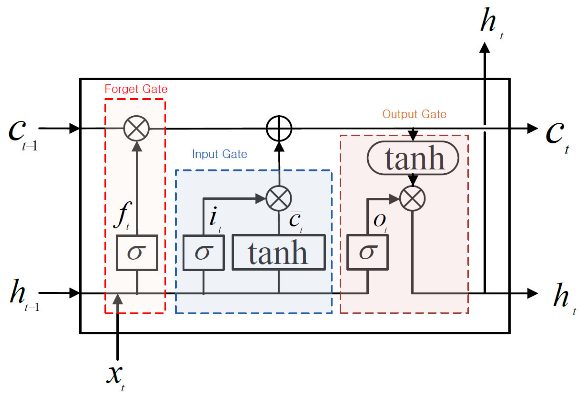
2.1.3. Long Short-Term Memory (LSTM)

LSTM is a model of sequential data that improves the long-term memory loss problem of Simple RNN [26]. As shown in Figure 3, LSTM consists of forget gate, input gate and output gate. The key to LSTM is having a cell state. The horizontal line from $c_{t-1}$ to $c_t$ located at the top of Figure 3 is called the cell state that penetrates the entire time series data through a simple linear operation. Because of this structure, time series information is continuously transferred to the next time step without memory loss.

$$f_t=\mathsf{\sigma }\left(W_f·\left[h_{t-1}, x_t\right]+b_f\right)$$

(2)

$$i_t=\mathsf{\sigma }\left(W_i·\left[h_{t-1}, x_t\right]+b_i\right)$$

(3)

$${\overline{c}}_t=\tan \mathrm{h}\left(W_c·\left[h_{t-1}, x_t\right]+b_c\right)$$

(4)

$$c_t=f_t c_{t-1} + i_t {\overline{c}}_t$$

(5)

$$o_t=\mathsf{\sigma }\left(W_o·\left[h_{t-1}, x_t\right]+b_o\right)$$

(6)

$$h_t={\mathrm{o}}_t\tanh \left(c_t\right),$$

(7)

where $f_t$, $i_t$ and $o_t$ are the forget, input and output gates at time $t$, respectively; $W_f$, $W_i$ and $W_o$ are weights mapped to hidden layers for forget, input and output gates; $b_f$, $b_i$ and $b_o$ are bias vectors; $\tanh (\cdot )$ is hyperbolic tangent function; $c_{t-1}$ and $c_i$ are the cell states of the previous time step and the next time step.

2.1.4. Bidirectional LSTM (Bi-LSTM)

The hidden layer neural network with Bi-LSTM [27], as shown in Figure 4, can expect high perceived performance because it learns both forward and backward directions of input sequence weights compared to uni-direction, which only learns forward direction [28].

2.1.5. Gated Recurrent Unit (GRU)

GRU plays a similar role as LSTM but it is computationally efficient because it consists of a simpler structure. This reduced the calculation of cell state used by conventional LSTM. GRU is a simplified form of three gates of LSTM. As shown in Figure 5, the input gate and forget gate are combined and simplified into an update gate [29]. GRU only has two types such as update gate and reset gate and removed cell state. GRU uses the activation function twice and the tanh function once. Thus, GRU has fewer parameters than LSTM and is faster to train but it is capable of long-term memory such as LSTM.

$$r_t=\mathsf{\sigma }\left(W_r·\left[h_{t-1}, x_t\right]+b_r\right)$$

(8)

$$z_t=\mathsf{\sigma }\left(W_z·\left[h_{t-1}, x_t\right]+b_z\right)$$

(9)

$${\overline{h}}_t=\tan \mathrm{h}\left(W·\left[h_{t-1}, x_t\right]+b\right)$$

(10)

$$h_t=\left(1-z_t\right)h_{t-1} + z_t {\overline{h}}_t$$

(11)

where $r$ and $z$ are the reset and update gates, respectively. Reset gate aims to reset past data and outputs a value between 0 and 1, which is the value of how much past data will be reset through the activation function. The update gate determines the rate of past and present information updates and the output value $z_t$ determines the amount of data to be exported at this point in time. $1-z_t$ is the amount of data to be forgotten.

2.2. Application of Models

In this study, we want to compare the accuracy and performance of the prediction of flow rates by selecting five models suitable for high flow rate prediction using time series data among various deep learning techniques. The time series flow rates are used as input and output data, which is the runoff data of the stream. These time series data are very important for flood warning and its defense in the field of water resources. The purpose of this study is to accurately predict future stream flow rates by utilizing one time series flow rate, which is one-variate data, as input data.

We propose deep learning techniques suitable for extreme flood forecasting to prepare for extreme flooding in water resources and to establish an accurate flood warning system and propose the length of input learning data through this study to ensure adequate accuracy. First of all, due to the nature of the time series data, it is necessary to calculate the appropriate sequence length that the relevant data has. Therefore, we would like to select the best deep learning technique for predicting time series data most recently to determine sequence length for the appropriate flow rates in stream with large flow fluctuations. In addition, an applicable deep learning model can be proposed by calculating the predicted accuracy of flow rate data with large flow fluctuations by combining suitable deep learning models based on previously developed models according to sequence length determined. Finally, in order to ensure the future prediction accuracy of the time series data with limited length, the accuracy and performance of the flow rate prediction according to the length of the time series data learned are calculated and compared. If the length of observational data to be entered into the DNN model is relatively short and it is feared that there will be significant errors in learning and forecasting, a measure should be devised to derive the best high flow rate forecast results using only the observed data.

3. Study Area and Data

3.1. Study Area

The Han River, in a highly urbanized Han River basin, was selected (Figure 6). The Han River basin is located in the central part of the Korean Peninsula over a latitude of 36°30′ N to 38°55′ N and longitude 126°24′ E to 129°02′ E. As shown in

Table 1. Summary of site characteristics.

Length of River (km)	Basin Area $\left({\mathbf{km}}^2\right)$	Mean Rainfall (mm/Year)	Mean Streamflow $\left({\mathbf{m}}^3/\mathbf{s}\right)$
494.44	25,953.60	1313.42	355.97

, the Han River has a basin area of 25,953.60 ${\mathrm{km}}^2$ (excluding the 9816.81 ${\mathrm{km}}^2$ area of North Korea) and is the largest river in South Korea with the total length of 494.44 km, an average width of 72.35 km and the shape coefficient of 0.146. The Han River basin is a multi-type basin that is a mixture of dendritic form and facsimile form. Historically, the Han River was channelized with its sinuosity demolished as a result of flow modifications, because of the urbanization of the Han River basin [30].

The primary land cover types in year 2003 were 5.4% agricultural land, 25.6% forest, 8.8% river, 39.4% vacant land, 2.5% park and 18.3% urban area [30]. Table 1 gives a summary of the channel characteristics. The channelized reach of average river width 1300 m has an average slope of 0.0016% on the downstream reach of the Han River basin [31,32].

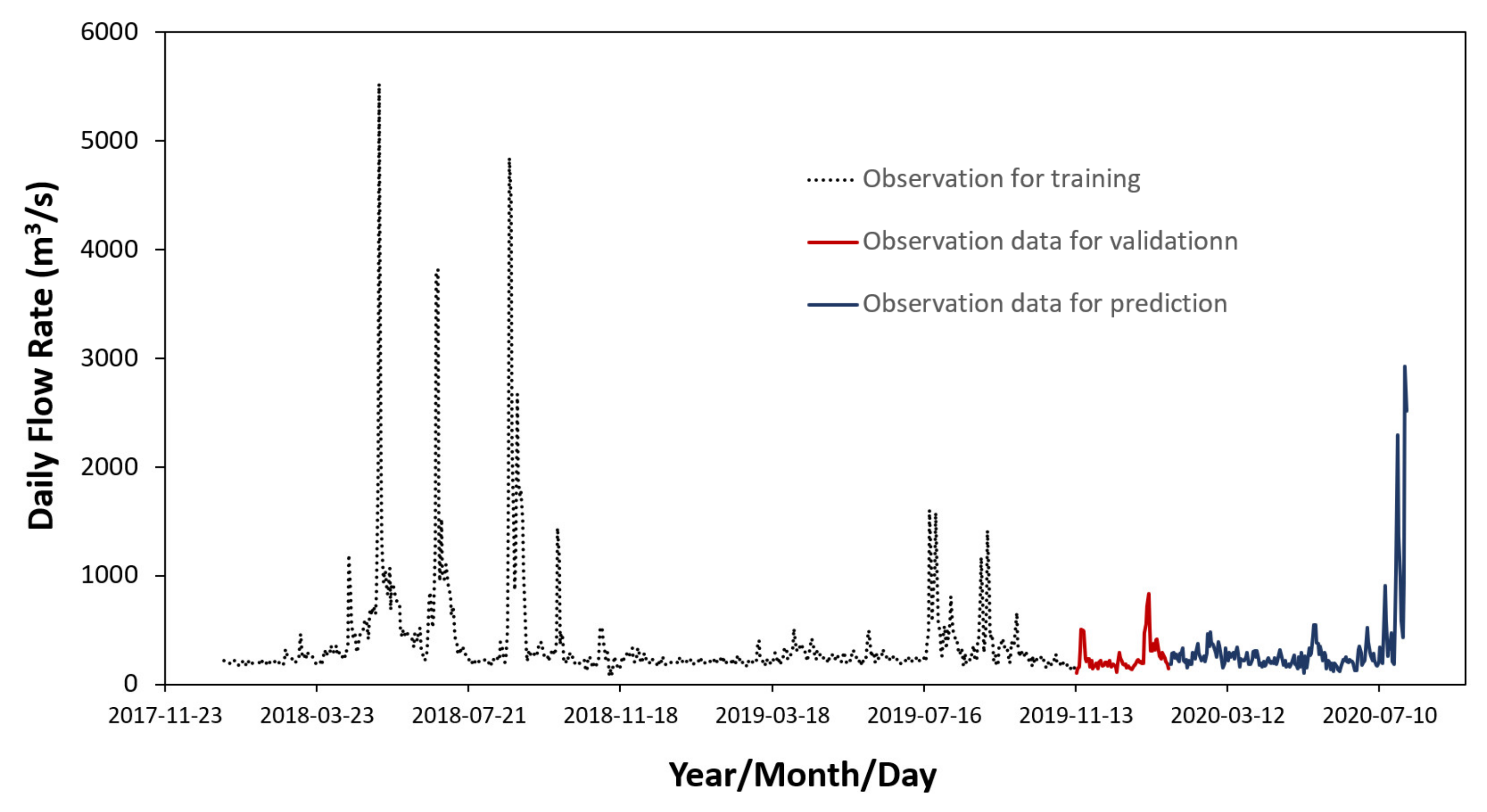
3.2. Hydrologic Data

In this study, the runoff data of Hangang Bridge Station (Figure 6), which is observed by the Ministry of Environment, Korea, were used. Flow data from the flow monitoring station were obtained using the data from the WAMIS website of the Ministry of Environment [33].

The average annual precipitation from 2010 to 2019 was 1313.42 mm, with 60% of the precipitation falling during the monsoon season of July to September based on the rainfall data provided by the website of Korea Meteorological Administration [35]. Thus, since seasonal rainfall is concentrated during the summer, the amount of runoff also increases rapidly at that time. The longer the data, the better the results. However, in this study, the deep learning models were validated using relatively short data of 2 years and 7 months to determine the critical size of learning data by reducing the length of data to be applied to model predictions. As shown in

Table 2. Statistical characteristics of daily flow rates at the Hangang Bridge (period: 2018–2020).

Minimum Flow Rate $\left({\mathbf{m}}^3/\mathbf{s}\right)$	Maximum Flow Rate $\left({\mathbf{m}}^3/\mathbf{s}\right)$	Average Flow Rate $\left({\mathbf{m}}^3/\mathbf{s}\right)$	Coefficient of Flow Fluctuation (CFF)	Standard Deviation of Flow Rate $\left({\mathbf{m}}^3/\mathbf{s}\right)$
78.60	5527.19	355.97	70.32	425.84

and Figure 7, the observed daily flow rates from the Hangang Bridge station were based on real-time observed data from 1 January 2018 to 31 July 2020. In order to analyze the characteristics of flow rates, the average, the minimum and the maximum flow rate were statistically analyzed as shown in Table 2. The flow rate variation is 425.84 ${\mathrm{m}}^3/\mathrm{s}$, which is larger than the average flow rate of 355.97 ${\mathrm{m}}^3/\mathrm{s}$ and the seasonal runoff changes at this site are very large. Before the multi-purpose dams were built in the Han River, the Coefficient of Flow Fluctuation (CFF) was 390: the CFF is defined as the ratio of annual maximum flow rate and annual minimum flow rate [36]. Large-scale multi-purpose dams were built upstream to control the flow rate: after constructing multi-purpose dams for flood control and securing water supply, the CFF has been dramatically lowered to 70.32. However, the seasonal changes are still very large compared to the CFF in foreign rivers (e.g., 3 for the Mississippi River, 8 for the Thames River, 18 for the Rhine River and 30 for the Nile River), which have a constant flow rate throughout the year [36].

As shown in Figure 7, the selected time series data were used for three stages of calculation and prediction. The distribution of the length of the entire time series data was 80% used as learning data. The remaining 20% of the data length was used to evaluate the accuracy of the model. The blue solid line in Figure 7 was allocated as forecast data. However, the last 10% of the time series (i.e., validation data) out of 80% of the learning data distributed was used as verification data to evaluate the adequacy of training in the learning process and shown in Figure 7 as a red solid line. Therefore, the training data used in the actual deep learning model corresponds to the portion of the 80% data length allocated to the learning, excluding 10% of the verification data. The validation data is indicated by a red solid line as shown in Figure 7.

3.3. Composition of Models

In this study, Python version 3.7.7 [37], an open-source program language and TensorFlow version 2.1.0 [38], a representative machine learning library, were used. As shown in

Table 3. Composition and hyperparameters of models.

Model	Activation Function	Input Layer	Hidden Layer 1	Dropout	Hidden Layer 2	Dense Layer 1	Dense Layer 2
CNN	ReLU	Conv1D	Conv1D 5 units/ Max Pooling 5 units	0.25	Flatten 10 units	25 units	1 unit
Simple RNN	ReLU	Simple RNN	Simple RNN 50 units	0.25	Simple RNN 50 units	25 units	1 unit
LSTM	ReLU	LSTM	LSTM 50 units	0.25	LSTM 50 units	25 units	1 unit
Bi-LSTM	ReLU	Bi-LSTM	Bi-LSTM 50 units	0.25	Bi-LSTM 50 units	25 units	1 unit
GRU	ReLU	GRU	GRU 50 units	0.25	GRU 50 units	25 units	1 unit

, the deep learning models used in the study were CNN, simple RNN, LSTM, Bi-LSTM and GRU. For each model, the form of the neuron and the number of units comprising each layer of it are shown in Table 3. The composition of the remaining models except CNN consists of 1 input layer, 2 hidden layers, 1 dropout and 2 dense layers and the detailed composition and hyperparameters of each model is given in Table 3.

One-time learning of the entire training data entered into the models was defined as epoch and the results of the model calculation were sufficiently convergent after 600 epochs of learning. The Adam optimizer was used to achieve convergent results while the model performed the learning and the cost function was using Mean Squared Error (MSE).

3.4. Model Performace Indicators

To evaluate the performance and accuracy of the deep learning models, model evaluation criteria from Equations (12)–(16) were used. The closer the mean absolute error (MAE), mean square error (MSE) and mean square error (RMSE) are to 0, the better the performance of the model. The closer Nash-Sutcliffe model efficiency coefficient (NS) and Coefficient of determination ($R^2$) are to 1, the better the performance of the model.

(1)

Mean Absolute Error (MAE)

MAE measures the average magnitude of the errors in a set of predictions, without considering their direction. It is the average over the test sample of the absolute differences between prediction and actual observation where all individual differences have equal weight [39].

$$\mathrm{MAE}=\frac{1}{N}{{\displaystyle \sum }}_{i=1}^N\left|x_i-y_i\right| ,$$

(12)

where $x_i$ are the observed values of the variables, $y_i$ are the predicted values and $N$ is the number of data.

(2)

Mean Squared Error (MSE)

MSE measures the average of the squares of the errors, that is, the average squared difference between the predicted value and the actual observation value [39].

$$\mathrm{MSE}=\frac{1}{N}{{\displaystyle \sum }}_{i=1}^N{\left(x_i-y_i\right)}^2.$$

(13)

(3)

Root Mean Squared Error (RMSE)

RMSE is a quadratic scoring rule that also measures the average magnitude of the error. It is the square root of the average of squared differences between prediction and actual observation [39,40,41].

$$\mathrm{RMSE}=\sqrt{\frac{{{\displaystyle \sum }}_{i=1}^N{\left(x_i-y_i\right)}^2}{N}}.$$

(14)

(4)

Coefficient of determination

The coefficient of determination $R^2$ is a measure of the goodness of fit of a statistical model [39,42,43].

$$R^2=1-\frac{{{\displaystyle \sum }}_{i=1}^N{\left(x_i-{\widehat{y}}_i\right)}^2}{{{\displaystyle \sum }}_{i=1}^N{\left(x_i-\overline{x}\right)}^2},$$

(15)

where ${\widehat{y}}_i$ are the predicted values from a statistical model and $\overline{x}$ is the mean of observed values of the variables.

(5)

Nash-Sutcliffe model Efficiency coefficient (NSE)

NS is used to quantify how well a model simulation can predict the outcome variable [39,40,42,43].

$$\mathrm{NSE}=1-\frac{{{\displaystyle \sum }}_{i=1}^N{\left(x_i-y_i\right)}^2}{{{\displaystyle \sum }}_{i=1}^N{\left(x_i-\overline{x}\right)}^2}.$$

(16)

As shown in

Table 4. Performance ratings for adopted statistics.

Performance Rating	${\mathit{R}}^2$	$\mathbf{NSE}$
Very good	$0.75<R^2\le 1.00$	$0.75<\mathrm{NSE} \le 1.00$
Good	$0.65<R^2\le 0.75$	$0.65<\mathrm{NSE}\le 0.75$
Satisfactory	$0.50<R^2\le 0.65$	$0.50<\mathrm{NSE} \le 0.65$
Unsatisfactory	$R^2\le 0.50$	$\mathrm{NSE} \le 0.50$

, it is not appropriate to adopt model result if $R^2$ and $\mathrm{NSE}$ are less than 0.5; if $R^2$ and $\mathrm{NSE}$ are greater than 0.5 and less than 0.65, it is possible to adopt model; If the $R^2$ and $\mathrm{NSE}$ are greater than 0.65 and less than 0.75, it is good for adoption; Also if $\mathrm{NSE}$ and $R^2$ is above 0.75, it is very good to adopt the model [22,39,42,44].

4. Results

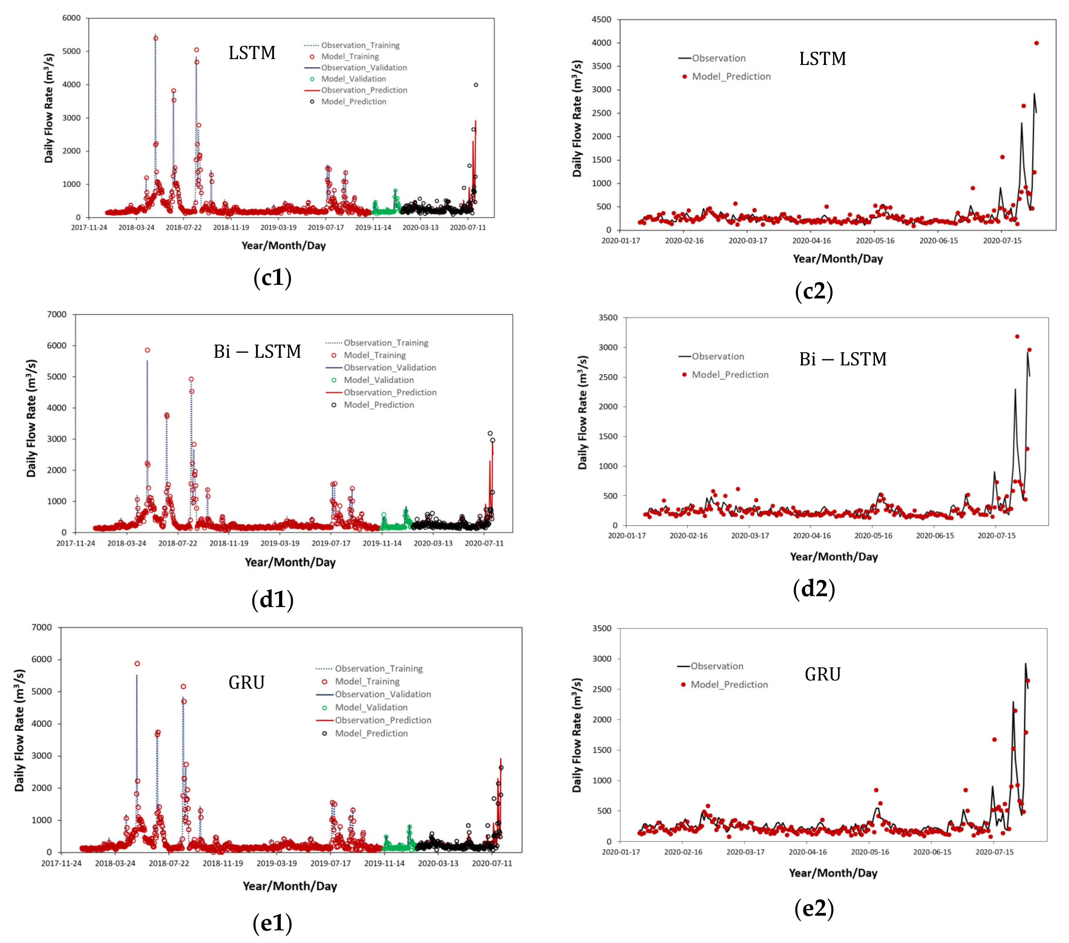
4.1. Results on Traning, Validation and Prediction Using Various Time Series Deep Learning Models

The learning and predicted results for 5 deep learning models (CNN, Simple RNN, LSTM, Bi-LSTM and GRU) for time series data are shown in Figure 8 and

Table 5. Performance comparison of models.

Model	Computational State	MAE	MSE	RMSE	${\mathit{R}}^{\mathbf{2}}$	NSE
CNN	Training	113.53	133.55	11.56	0.557	0.557
	Validation	69.37	492.59	22.19	0.512	0.525
	Prediction	92.83	101.53	10.08	0.526	0.527
Simple RNN	Training	107.32	6633.79	81.45	0.864	0.868
	Validation	93.10	5951.47	77.15	0.133	0.348
	Prediction	123.89	3315.69	57.58	0.418	0.435
LSTM	Training	25.06	74.89	8.69	0.994	0.994
	Validation	57.69	154.21	12.42	0.473	0.477
	Prediction	114.93	4.72	2.17	0.394	0.394
Bi-LSTM	Training	27.61	285.04	16.88	0.994	0.994
	Validation	44.69	293.10	17.12	0.748	0.752
	Prediction	102.68	672.41	25.93	0.466	0.469
GRU	Training	50.90	2201.17	46.92	0.984	0.984
	Validation	66.63	2643.39	51.41	0.513	0.576
	Prediction	102.19	753.54	27.45	0.691	0.693

. The results of the CNN model were not well achieved, as shown in Figure 8(a1,a2), respectively and the predictions for high flow rate were not well predicted. However, the forecasts of low flow rates were adequately predicted. The training and prediction results of simple RNN were improved than those of CNN but still under-calculated in high flow rates (Figure 8(b1)) and the prediction results were rather overestimated in high flow rates (Figure 8(b2)). As shown in Figure 8(c1,c2) and Table 5, the results of the LSTM model showed a sharp improvement in accuracy ($\mathrm{NSE}=0.994$) in the learning outcomes of the high flow rates but the results of forecast of the high flow rates were still overestimated. The learning results of Bi-LSTM and GRU were very accurate with $\mathrm{NSE}=0.984-0.994$ and, the predicted results for GRU, with high accuracy ($\mathrm{NSE}=0.693$) in all flow rate ranges (Table 5). The results of the prediction of Bi-LSTM were well predicted for most flow rate ranges, as shown in Figure 8(d2) but the predictions of high flow rates were somewhat overestimated and the accuracy was reduced. Therefore, based on the results of this study, the GRU model was able to predict both learning ($\mathrm{NSE}=0.984$) and forecasting ($\mathrm{NSE}=0.693$) with high accuracy in the case of the Han River with large flow fluctuations (Figure 8(e1,e2)).

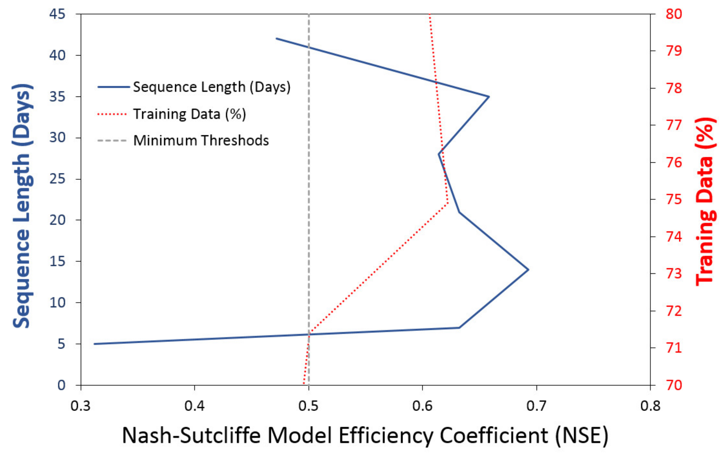
4.2. Training and Prediction Results of Sequence Length Variation Using GRU

Deep learning calculations were performed for sequence length using all deep learning models but reflecting the results of Section 4.1, only the results for sequence length for GRU, the model with the best prediction results, were specified in Figure 9 and

Table 6. Performance comparison of GRU with variation of sequence length.

Sequence Length (Days)	Computational State	MAE	MSE	RMSE	${\mathit{R}}^{\mathbf{2}}$	NSE
4	Training	75.33	2534.94	50.35	0.961	0.961
	Validation	85.25	3889.03	62.36	0.257	0.389
	Prediction	123.63	3309.35	57.53	0.291	0.312
7	Training	42.84	534.27	23.11	0.986	0.986
	Validation	62.42	1158.18	34.03	0.612	0.636
	Prediction	101.69	979.24	31.29	0.628	0.632
14	Training	50.90	2201.17	46.92	0.984	0.984
	Validation	66.63	2643.39	51.41	0.513	0.576
	Prediction	102.19	753.54	27.45	0.690	0.693
21	Training	31.38	3.66	1.91	0.975	0.975
	Validation	62.74	17.74	4.21	0.549	0.549
	Prediction	101.69	979.24	31.29	0.628	0.632
28	Training	31.84	180.78	13.45	0.992	0.992
	Validation	66.18	707.03	26.59	0.515	0.534
	Prediction	104.28	833.30	28.87	0.611	0.614
35	Training	25.78	10.05	3.17	0.994	0.994
	Validation	56.21	593.75	24.37	0.507	0.522
	Prediction	95.73	0.10	0.32	0.658	0.658
42	Training	41.26	368.71	19.20	0.988	0.988
	Validation	52.11	319.11	52.11	0.700	0.705
	Prediction	104.13	147.80	12.16	0.471	0.472

. Thus, the model used for the predictions mentioned in this section was GRU and all results were calculated after learning 600 epochs, as shown in Figure 9 and Table 6.

As shown in Figure 9, training data used 72% of the total number of data and 8% of the data was used as validation data. And the other 20% of the data was used as prediction data. Comparing NSEs to the model suitability in Table 3, NSEs were calculated in the range of 0.994 to 0.961 as a result of learning. When the sequence length was 7 days and 14 days, learning results tended to overfit and NSE values were in the range of 0.507 to 0.549 in the validation data: due to the small number of data entered in the validation data, the NSE values were somewhat small but it was determined that there was no significant problem in verifying the performance of the overall model.

If the sequence lengths were within 7 to 35 days, the predicted NSE results were 0.632 to 0.693 and the predicted results were calculated to be sufficiently reliable (Table 6). However, when the sequence lengths were 4 days and 42 days, the NSE values dropped sharply, respectively, to 0.312 and 0.472 and the model results deteriorated. Therefore, it was considered appropriate to select the appropriate sequence length from the GRU model for a range of 7 to 35 days in the Han River with large seasonal fluctuations like this study site. $R^2\mathrm{s}$ also had the same or slightly smaller value as NSEs, as shown in Table 6. Due to the large change in flow rate of the stream, the remaining performance criteria (such as MAE, MSE and RMSE) of the model had large values even after the completion of the learning but if analyzed by the results of the model’s training accuracy and prediction accuracy, it can be seen that the results were sufficiently converged.

As shown in (a4)–(c4) of Figure 9, the $R^2$ values were shown to be capable of predicting a reasonable level of high flow rates, although some under- or overestimated, as the sequence length increased from 7 days to 21 days. For intermediate or low flow rates, all results were predicted to be at a high level of accuracy (Figure 9(a2–c2)). Therefore, we excluded the case where the sequence length is 7 days to avoid overfitting problems by aggregating the results of this study. Using the sequence length 14 days data, a high accuracy prediction results were obtained for all flow rate ranges.

4.3. GRU Performance with Changes in Length of Training Data and Prediction Data

In this section, we observed the accuracy of the predicted flow rate by fixing the length of the prediction data at 188 and reducing the size of the training data: the size of the prediction data presented in

Table 7. Comparison of GRU performance with changes in length of training data and prediction data.

Training Data (%)	Prediction Data (%)	Computational State	MAE	MSE	RMSE	${\mathit{R}}^{\mathbf{2}}$	NSE
80.0	20.0	Training	30.22	300.28	17.33	0.991	0.991
		Prediction	103.13	527.31	22.96	0.604	0.606
74.9	25.1	Training	17.01	8.06	2.84	0.995	0.995
		Prediction	98.29	117.27	10.83	0.622	0.622
71.4	28.6	Training	10.91	9.04	3.01	0.993	0.993
		Prediction	101.42	876.86	29.61	0.501	0.501
66.8	33.2	Training	8.23	2.33	1.53	0.997	0.997
		Prediction	102.15	1093.35	33.07	0.479	0.484

was from 26 January 2020 to 31 July 2020, with the total number of data lengths fixed at 188. The maximum size of the training data was from 1 January 2018 to 25 January 2020. By reducing the number of training data from January 2018, a total of four time series learning data were prepared. Using GRU model, the accuracy of prediction according to the size of the training data was observed. As shown in Table 7, the number of training data and the number of prediction data were added to calculate the ratio of each training data and prediction data. Therefore, the ratio of training data entered into GRU was reduced to 80.0%, 74.9%, 71.4% and 66.8%, respectively but the absolute size of prediction data was the same for all cases, at 188: the proportion of prediction data in the four groups of data increased to 20.0%, 25.1%, 28.6% and 33.2%, respectively.

The results calculated from 600 epochs using the GRU model at the sequence length of 14 days with the same model input conditions were shown in Table 7. The calculation for validation was not performed because the main purpose of this calculation was to find the critical input size of the training data. Only training and prediction calculations were performed to ensure sufficient number of training data.

As shown in Table 7, even if the proportion of training data decreased from 80% to 74.9%, NSE increased from 0.606 to 0.622 to gain confidence in the forecast results. However, further reducing the size of training data to below 71.41% caused NSE to deteriorate rapidly in the range of 0.501 to 0.484, making the forecast results unreliable.

In the case of training data in Figure 10(a1,b1), high flow rate data were included in the learning data, which also allowed the prediction of high flow rate results as shown in Figure 10(a2,b2). However, if the training data continued to be shortened and the high flow rate data were removed from the learning input, the prediction flow rates were gradually underestimated as shown in Figure 10(c4,d4). Nevertheless, for learning materials entered into the model as shown in Figure 10(c3,d3), the learning results were still very high (NSE = 0.993–0.997). Thus, the input ratio of the data being trained based on the results of this section must be entered in sizes of 74.9% to 80.0%.

Therefore, these results may suggest the minimum input size of data in the establishment of flood warning system for urban rivers, on the contrary, the size of predictable flood warning results can be appropriately determined to establish an effective flood warning system for urban development streams where there is not enough observation data.

5. Discussion

5.1. Comparison with Previous Studies

• Most of the DNN studies used in previous water resources engineering [10,11,12,13,14,15,16,17,18,19,20,21,22] were mainly used by RNN, Bi-LSTM and LSTM models to predict time series data. The GRU model had similar accuracy as the LSTM model but as shown in Figure 5, the GRU model is simplified by omitting the cell state calculation rather than using 3 gates in the LSTM model and can effectively calculate the large flow rates.
• As seen in previous studies [10,11,12], most applications of deep learning technology in the field of water resources engineering were focused on predicting the water levels in streams and the inflows into dams with small variation in hydraulic variables. When DNN models were learning time series data with very high seasonal fluctuations, relatively accurate predictions were possible for low flow rates but the accuracy at high flow rates were significantly reduced. Thus, unlike previous studies for flood runoff prediction, if the variation between the minimum and maximum values of the time series data is very large, the predicted accuracy of the time series data becomes very inaccurate and vulnerable. In this study, LSTM and GRU models were able to achieve better results than other RNN models when the seasonal fluctuations in the flow rate of urban streams were very large. Among them, GRU model results were the best.
• In most areas of water resources engineering [9,13,14,15,16,17,18,19,20,21,22], the time series data of any length were utilized as input data without proper consideration of the sequence length of the data in the calculation of the DNN models, which can predict water levels and flow rates. However, it is essential to verify the change in accuracy according to the sequence length of time series data that directly affects the forecast results. In this study, NSE was selected as 0.5 as the minimum threshold for sequence length. The range of sequence length applicable to the Han River ($CFF=70.32)$, which had a very large flow fluctuation, was 7 to 35 days and in the case of 14 days, the most optimal prediction of the flow rates could be obtained.
• When the length of the observation data of flow rates is not sufficiently secured, the length of the minimum input time series flow data to be learned must be determined in order to predict the flood flow rates for a specified period of time with minimum accuracy ($NSE\ge 0.5)$. In previous studies [10,11,12,13,14,15,16,17,18,19,20,21,22], the lengths of training data and forecast data were arbitrarily determined. But in this study, if the length of the training data was determined within the range of 74.9% to 80% of the total data length, the forecast results were also accurately predicted in high flow rates.

As discussed above, in most cases, where deep learning is applied to the water resources engineering to predict flow rates or water elevations, the sequence length and the length of learning data were selected by entering random lengths of data without clear evidence. Therefore, this study could present very meaningful results that could quantitatively determine the input length of data in the Han River, an urban stream with large seasonal flow rate fluctuations.

5.2. Critical Conditions of Deep Learning to Ensure Reliability

Through this study, the critical conditions for prediction that have secured reliability in urban streams where seasonal changes in flow rates such as the Han River are very large could be proposed as shown in Figure 11. The criteria for the performance evaluation of learning and forecasting models were NSE. By varying the sequence length and training data size (%) and by plotting the entered learning results and predicted results, the performance evaluation results of the deep learning model can be defined as the criteria that can be used in flood forecasting systems in the future as shown in Figure 11. Based on Table 4, the minimum threshold of available NSE was set to 0.5. If the two variable relationships are illustrated as shown in Figure 11, NSE is greater than 0.5 and, if the maximum is reached, is estimated to be the input condition of the most effective deep learning model for accurate flow rate prediction: it is possible to accurately predict the flow rate by selecting the sequence lengths between 7 and 21 days and using input data of 74.9% to 80% for training data size. In addition, as shown in Section 4.3, high flow rate data should be included without being removed from the learning data entered into deep learning.

The process of sensitivity analysis calculated the accuracy by changing the data length to determine the appropriate sequence length. This result was derived for rivers with large flow rates and large flow fluctuations, such as the Han River and provided a basis for engineering judgment to predict flow rates due to seasonal changes. However, sensitivity analysis on input length and sequence length of data applicable to various streams needs further research in the future.

6. Conclusions

Recently, due to climate change and urban development projects around rivers, the development of flood prediction technology for urban streams has been studied in various ways. Flood prevention measures are being prepared in terms of creating a safe and sustainable waterfront space because of concerns over flooding in cities caused by rapid increase in floods due to urbanization. In order to achieve this goal, accurate prediction of high flow rates must be possible, especially for rivers with severe seasonal changes in flow rates, it is imperative to prepare a flood warning system. Therefore, in this study, 5 models of deep learning (i.e., CNN, simple RNN, LSTM, Bi-LSTM and GRU) were applied to evaluate the accuracy of high flow rate forecasts to suggest the best deep learning technique suitable for predicting continuous time series data for accurate high flow rate forecasting.

In the case of the Han River flowing through Seoul, Korea, GRU was chosen as a deep learning model suitable for cases where seasonal fluctuations in flow rate are up to 70.32 times. It is also important to set a sequence length that accurately reflects the trend of the previous time series in order to predict the exact time series flow. Therefore, the sequence length was appropriate between 7 and 35 days by calculating the predicted accuracy according to the various sequence lengths. However, if the sequence length of 7 days was selected, overfitting occurred in the learning process, so if the sequence length of 14 days is used in this study, the overfitting that can occur during the training process could be minimized. Finally, for the prediction of the time series flow rate for a given period, the minimum length (%) of the training data could be proposed at 74.9–80%. In this case, the reliability of the forecast results could be obtained.

The results of this study examined the accuracy of the predicted flow rates according to the length of the input flow data in urban streams, where the flow rate increases and fluctuates greatly due to urbanization. If the minimum length of the input data is obtained, the use of deep learning technology compared to the results calculated by the traditional CFD models is evaluated as an important achievement as it can effectively predict the flow rates quickly and accurately.

References

1. Lee, K.S. Rehabilitation of the Hydrologic Cycle in the Anyangcheon Watershed, Sustainable Water Resources Research Center; Ministry of Education, Science and Technology: Seoul, Korea, 2007. [Google Scholar]
2. Lee, K.S.; Chung, E.S. Development of integrated watershed management schemes for an intensively urbanized region in Korea. J. Hydro Environ. Res. 2007, 1, 95–109. [Google Scholar] [CrossRef]
3. Henonin, J.; Russo, B.; Mark, O.; Gourbesville, P. Real-time urban flood forecasting and modelling—A state of the art. J. Hydroinform. 2013, 15, 717–736. [Google Scholar] [CrossRef]
4. Carter, R.W.; Godfrey, R.G. Storage and Flood Routing; Manual of Hydrology: Part 3. Flood-Flow Techniques, Geological Survey Water-Supply Paper 1543-B, Methods and Practices of the Geological Survey; US Department of the Interior: Washington, DC, USA, 1960. [Google Scholar]
5. Moussa, R.; Bocquillon, C. Approximation zones of the Saint-Venant equations for flood routing with overbank flow. Hydrol. Earth Syst. Sci. 2000, 4, 251–260. [Google Scholar] [CrossRef] [Green Version]
6. Kim, B.; Sanders, B.; Famiglietti, J.S.; Guinot, V. Urban flood modeling with porous shallow-water equations: A case study of model errors in the presence of anisotropic porosity. J. Hydrol. 2015, 523, 680–692. [Google Scholar] [CrossRef] [Green Version]
7. Biscarini, C.; Francesco, S.D.; Ridolfi, E.; Manciola, P. On the simulation of floods in a narrow bending valley: The Malpasset Dam break case study. Water 2016, 8, 545. [Google Scholar] [CrossRef] [Green Version]
8. Nkwunonwo, U.C.; Whitworth, M.; Baily, B. A review of the current status of flood modelling for urban flood risk management in the developing countries. Sci. Afr. 2020, 7, 1–15. [Google Scholar] [CrossRef]
9. Ghumman, A.R.; Ghazaw, Y.M.; Sohail, A.R.; Watanabe, K. Runoff forecasting by artificial neural network and conventional model. Alex. Eng. J. 2011, 50, 345–350. [Google Scholar] [CrossRef] [Green Version]
10. Kim, S.; Tachikawa, Y. Real-time river-stage prediction with artificial neural network based on only upstream observation data. J. Jpn. Soc. Civ. Eng. Ser. B1 Hydraul. Eng. 2018, 74, I_1375–I_1380. [Google Scholar] [CrossRef]
11. Tran, Q.-K.; Song, S.-K. Water level forecasting based on deep learning: A use case of Trinity River-Texas-the United States. J. KIISE 2017, 44, 607–612. [Google Scholar] [CrossRef]
12. Yoo, H.; Lee, S.O.; Choi, S.; Park, M. A study on the data driven neural network model for the prediction of time series data: Application of water surface elevation forecasting in Hangang River Bridge. J. Korean Soc. Disaster Secur. 2019, 12, 73–82. [Google Scholar]
13. Elumalai, V.; Brindha, K.; Sithole, B.; Lakshmanan, E. Spatial interpolation methods and geostatistics for mapping groundwater contamination in a coastal area. Environ. Sci. Pollut. Res. 2017, 21, 11601–11617. [Google Scholar] [CrossRef] [PubMed]
14. Kumar, D.N.; Raju, K.S.; Sathish, T. River flow forecasting using recurrent neural networks. Water Resour. Manag. 2004, 18, 143–161. [Google Scholar] [CrossRef]
15. Firat, M. Comparison of artificial intelligence techniques for river flow forecasting. Hydrol. Earth Syst. Sci. 2008, 12, 123–139. [Google Scholar] [CrossRef] [Green Version]
16. Sattari, M.T.; Yurekli, K.; Pal, M. Performance evaluation of artificial neural network approaches in forecasting reservoir inflow. Appl. Math. Model. 2012, 36, 2649–2657. [Google Scholar] [CrossRef]
17. Chen, P.-A.; Chang, L.-C.; Chang, L.-C. Reinforced recurrent neural networks for multi-step-ahead flood forecasts. J. Hydrol. 2013, 497, 71–79. [Google Scholar] [CrossRef]
18. Park, M.K.; Yoon, Y.S.; Lee, H.H.; Kom, J.H. Application of recurrent neural network for inflow prediction into multi-purpose dam basin. J. Korea Water Resour. Assoc. 2018, 51, 1217–1227. [Google Scholar]
19. Zhang, D.; Peng, Q.; Lin, J.; Wang, D.; Liu, X.; Zhuang, J. Simulating reservoir operation using a recurrent neural network algorithm. Water 2019, 11, 865. [Google Scholar] [CrossRef] [Green Version]
20. Mok, J.-Y.; Choi, J.-H.; Moon, Y.-I. Prediction of multipurpose dam inflow using deep learning. J. Korea Water Resour. Assoc. 2020, 53, 97–105. [Google Scholar]
21. Zhang, D.; Lin, J.; Peng, Q.; Wang, D.; Yang, T.; Sorooshian, S.; Liu, X.; Zhuang, J. Modeling and simulating of reservoir operation using the artificial neural network, support vector regression, deep learning algorithm. J. Hydrol. 2018, 565, 720–736. [Google Scholar] [CrossRef] [Green Version]
22. Apaydin, H.; Feizi, H.; Sattari, M.T.; Colak, M.S.; Shamshirband, S.; Chau, K.-W. Comparative analysis of recurrent neural network architectures for reservoir inflow forecasting. Water 2020, 12, 1500. [Google Scholar] [CrossRef]
23. Hatami, N.; Gavet, Y.; Debayle, J. Classification of time-series images using deep convolutional neural networks. In Proceedings of the Tenth International Conference on Machine Vision (ICMV 2017), Vienna, Austria, 13 April 2018; Volume 10696. [Google Scholar]
24. Wang, Z.; Oates, T. Encoding time series as images for visual inspection and classification using tiled convolutional neural networks. In Proceedings of the Twenty-Ninth AAAI Conference on Artificial Intelligence, Austin, TX, USA, 25–26 January 2015. [Google Scholar]
25. Bengio, Y.; Simard, P.; Frasconi, P. Learning long-term dependencies with gradient descent is difficult. IEEE Trans. Neural Netw. 1994, 5, 157–166. [Google Scholar] [CrossRef] [PubMed]
26. Hochreiter, S.; Schmidhuber, J. Long Short-Term Memory. Neural Comput. 1997, 9, 1735–1780. [Google Scholar] [CrossRef] [PubMed]
27. Graves, A.; Schmidhuber, J. Framewise phoneme classification with bidirectional LSTM and other neural network architectures. Neural Netw. 2005, 18, 602–610. [Google Scholar] [CrossRef] [PubMed]
28. Zhao, R.; Yan, R.; Wang, J.; Mao, K. Learning to monitor machine health with convolutional bi-directional LSTM networks. Sensors 2017, 17, 273. [Google Scholar] [CrossRef]
29. Cho, K.; Van Merrienboer, B.; Bahdanau, D.; Bengio, Y. On the Properties of Neural Machine Translation: Encoder–Decoder Approaches. In Proceedings of the SSST-8, Eighth Workshop on Syntax, Semantics and Structure in Statistical Translation, Doha, Qatar, 7 October 2014; pp. 103–111. [Google Scholar]
30. Seoul Metropolitan Government. Study on River Management by Universities; Seoul Metropolitan Government: Seoul, Korea, 2013.
31. Seoul Metropolitan Government. Statistical Yearbook of Seoul; Seoul Metropolitan Government: Seoul, Korea, 2004.
32. Ministry of Construction and Transportation. Master Plan for River Modification of the Han River Basin; Ministry of Construction and Transportation: Sejong City, Korea, 2002.
33. Water Resources Management Information System. Available online: http://www.wamis.go.kr (accessed on 1 August 2020).
34. Google Earth. Available online: http://www.google.com/maps (accessed on 15 October 2020).
35. Weather Data Portal. Available online: https://data.kma.go.kr/cmmn/main.do (accessed on 1 August 2020).
36. Lee, J.S. Water Resources Engineering; Goomibook: Seoul, Korea, 2008. [Google Scholar]
37. Anaconda. Available online: https://www.anaconda.com (accessed on 1 August 2020).
38. TensorFlow. Available online: https://www.tensorflow.org (accessed on 1 August 2020).
39. Moriasi, D.N.; Arnold, J.G.; Van Liew, M.W.; Bingner, R.L.; Harmel, R.D.; Veith, T.L. Model evaluation guidelines for systematic quantification of accuracy in watershed simulations. Soil Water Div. ASABE 2007, 50, 885–900. [Google Scholar]
40. Segura-Beltrán, F.; Sanchis-Ibor, C.; Morales-Hernández, M.; González-Sanchis, M.; Bussi, G.; Ortiz, E. Using post-flood surveys and geomorphologic mapping to evaluate hydrological and hydraulic models: The flash flood of the Girona River (Spain) in 2007. J. Hydrol. 2016, 541, 310–329. [Google Scholar] [CrossRef] [Green Version]
41. Kastridis, A.; Kirkenidis, C.; Sapountzis, M. An integrated approach of flash flood analysis in ungauged Mediterranean watersheds using post-flood surveys and unmanned aerial vehicles. Hydrol. Process. 2020, 34, 4920–4939. [Google Scholar] [CrossRef]
42. Narbondo, S.; Gorgoglione, A.; Crisci, M.; Chreties, C. Enhancing physical similarity approach to predict runoff in ungauged watersheds in sub-tropical regions. Water 2020, 12, 528. [Google Scholar] [CrossRef] [Green Version]
43. Chen, H.; Luo, Y.; Potter, C.; Moran, P.J.; Grieneisen, M.L.; Zhang, M. Modeling pesticide diuron loading from the San Joaquin watershed into the Sacramento-San Joaquin Delta using SWAT. Water Res. 2017, 121, 374–385. [Google Scholar] [CrossRef]
44. Chiew, F.; Stewardson, M.J.; McMahon, T. Comparison of six rainfall-runoff modelling approaches. J. Hydrol. 1993, 147, 1–36. [Google Scholar] [CrossRef]
Figure 1. Convolution Neural Network (CNN).
Water 12 03537 g001
Figure 2. Simple Recurrent Neural Network (Simple RNN).
Water 12 03537 g002
Figure 3. Long Short-Term Memory (LSTM).
Water 12 03537 g003
Figure 4. Bidirectional LSTM (Bi-LSTM).
Water 12 03537 g004
Figure 5. Gated Recurrent Unit (GRU).
Water 12 03537 g005
Figure 6. Map of the Han River basin in Korea (Google Earth [34]).
Water 12 03537 g006
Figure 7. Time series daily flow rates at the Hangang Bridge (period: 2018–2020).
Water 12 03537 g007
Figure 8. Observed and computed total time series flow rates (a1)–(e1) and prediction (a2)–(e2): (a1) and (a2) convolutional neural network (CNN); (b1) and (b2) simple recurrent neural network (RNN); (c1) and (c2) LSTM; (d1) and (d2) Bi-LSTM; and (e1) and (e2) gated recurrent unit (GRU).
Water 12 03537 g008aWater 12 03537 g008b
Figure 9. Observed and computed total time series flow rates (a1)–(c1), observed and computed predicted time series flow rates (a2)–(c2), R 2 for training (a3)–(c3) and R 2 for prediction (a3)–(c3) using GRU: (a1)–(a3) 7 days of sequence length; (b1)–(b3) 14 days of sequence length; (c1)–(c3) 21 days of sequence length.
Water 12 03537 g009aWater 12 03537 g009b
Figure 10. GRU performance with changes in length of training data and prediction data: (a1)–(d1) flow rates for training; (a2)–(d2) flow rates for prediction; (a3)–(d3) R 2 for training; (a4)–(d4) R 2   for prediction; (a1)–(a4) ratio of 80 to 20; (b1)–(b4) ratio of 74.9 to 25.1; (c1)–(c4) ratio of 71.4 to 28.6; (d1)–(d4) ratio of 66.8 to 33.2.
Water 12 03537 g010aWater 12 03537 g010b
Figure 11. Minimum threshold according to conditions sequence length and training data.
Water 12 03537 g011