Comparisons of Two Types of Particle Tracking Models Including the Effects of Vertical Velocity Shear

Abstract

In this study, two types of particle tracking models were presented to investigate the applicability in the two-dimensional solute mixing simulations. The conventional particle tracking model, denoted as PTM, was developed based on Fick’s law, which adopted the dispersion coefficient to calculate the random displacements. The other model is the particle dispersion model (PDM), which computes the shear dispersion process by dividing into two computation procedures as the shear translation and the vertical mixing. The PTM and the PDM included the effects of vertical profiles of velocity in the computation of dispersion coefficients and the shear translation step, respectively. The main difference between the two models is whether the shear dispersion process is reproduced using Fick’s law or the direct computation method. These differences were clearly revealed by comparing with the analytic solution of the advection-dispersion equation. The concentration curve resulting from the PTM shows the Gaussian curves, which were well-fitted with the analytic solution in both initial and Taylor periods. Meanwhile, the PDM presented skewed curves in the initial period and gradually turned to the symmetric shape in the Taylor period. The inherent differences of the two particle tracking models were scrutinized against the two-dimensional tracer test results, which show the non-Fickian mixing properties. The comparisons of concentration–time curves reveal that the PDM reproduced a more accurate shape of the curves than the results by the PTM by demonstrating skewed concentration curves.

1. Introduction

The increase of urban and industrial areas become a threat to aquatic environments by increasing possibilities of water pollution. Accurate predictions of pollutant mixing in rivers can reduce damage from water pollution accidents and secure public health by drawing essential information for disaster mitigation activities. The analysis of soluble pollutant mixing introduced in rivers is mainly conducted using two-dimensional (2D) models, as the vertical mixing is completed during a relatively short period [1,2]. The 2D mixing can be described based on the shear dispersion theory, as described in Figure 1, in which a pollutant cloud is stretched by shear flows in the longitudinal and transverse directions, and simultaneously diffused through flow depth by the turbulent diffusion [3]. In the 2D mixing model, the shear dispersion theory is modeled using Taylor’s study [4], in which the mass flux term derived from the depth-averaging process is assumed to be proportional to the concentration gradient based on Taylor’s assumption as follows [5].

$$-\frac{1}{h}{\displaystyle {\int }_0^h{u^{\prime }}_i{c}^{\prime }}dz=D_{ij}\frac{\partial C}{\partial x_j}$$

(1)

where $h$ is the flow depth; $z$ is the vertical direction; ${u^{\prime }}_i=u_i-{\overline{u}}_i$ and $c^{\prime }=c-C$ are the vertical fluctuations, which are subtractions of the depth-averaged values (${\overline{u}}_i$, $C$) from the vertical distributions ($u_i$, $c$), of velocity and concentration, respectively; and $D_{ij}$ are the dispersion coefficients in tensor notation. The relation shown in Equation (1) is only valid after the initial period, defined as below.

$$t_I=0.4\frac{h^2}{{\epsilon }_z}$$

(2)

where $t_I$ is the initial period, $h$ is flow depth, and ${\epsilon }_z$ is the vertical turbulent diffusion coefficient. Thus, in the 2D mixing simulations, determination of dispersion coefficients is one of the crucial concerns to conduct pollutant mixing simulations.

Several studies adopted empirical formulas obtained from tracer test results or theoretical approaches to determine the dispersion coefficient for solute transport simulations [6,7,8]. The empirical formulas of dispersion coefficient are presented as follows.

$$D_L=a_{L}h{u}^{*}$$

(3)

$$D_T=a_{T}h{u}^{*}$$

(4)

where $D_L$ and $D_T$ are the longitudinal and transverse dispersion coefficient, respectively; $a_L$ and $a_T$ are the empirical coefficients; and $u^{*}=\sqrt{gh{S}_f}$ is the shear velocity, in which $S_f$ is the energy slope, which can be obtained from Manning’s formula. In case of $D_T$, several studies have been reported that $a_T$ has a wide range of 0.15–3.0 according to hydraulic and geographical properties of rivers [9,10,11,12,13,14]. On the other hand, the theoretical formula of $D_L$ suggested by Elder [15] has been widely used for simulations instead of using the empirical formulas [2,16]. The theoretical value of $a_L$ is derived as 5.93 under the assumption of an infinitely wide width of straight channel and the log distribution in the longitudinal velocity shear. However, the theoretical value shows large discrepancies from the results of field studies, which suggested the value of $a_L$ to be in the range of 13–150 [17,18,19]. Instead of the aforementioned dispersion coefficient formulas, theoretical approaches reported by Fischer et al. [5] have been adopted to obtain dispersion coefficients by conducting triple integrations of vertical profiles of velocity [20]. The velocity-based method to calculate the dispersion coefficient is reported to adequately reproduce solute mixing in meandering channels [21]. Despite several studies to define the dispersion coefficients, it is still difficult to employ adequate values for two-dimensional solute mixing simulations following the Fick’s law.

The particle tracking method is an alternative to the grid-based solute transport models. The method is known as avoidable from the numerical oscillation and diffusion of the grid-based models [22]. Furthermore, the particle tracking approach is more suitable to simulate the transport of discontinuous properties of solute [23]. For these advantages, particle tracking simulations have been presented for solute transport in rivers [24] and estuaries [25,26]. The two-dimensional particle tracking model is derived from the mathematical analogy between the Fokker–Plank equation and the advection-dispersion equation [27]. Thus, the conventional particle tracking models adopted the dispersion coefficients into the random transport term following Fick’s law. However, several field studies have presented skewed concentration curves, which violate the Fickian mixing properties because of complexities of channel geometries [28,29,30]. To demonstrate these non-Fickian mixing behaviors, the particle tracking method has been adopted for two-dimensional mixing simulations [24,31].

In this study, the performance of two types of particle tracking models was evaluated by comparing the simulation results. The first model is derived from the conventional particle tracking model following Fick’s law. The second model is the particle dispersion model suggested by Park and Seo [31], in which the shear flow dispersion was reproduced using the sequential computations of shear translation and vertical diffusion instead of using the Fickian model. From the simulation results, the shapes of depth-averaged concentration curves were compared, and applicability of the two models was evaluated using Chatwin’s parameter [32] and statistical properties.

2. Model Descriptions

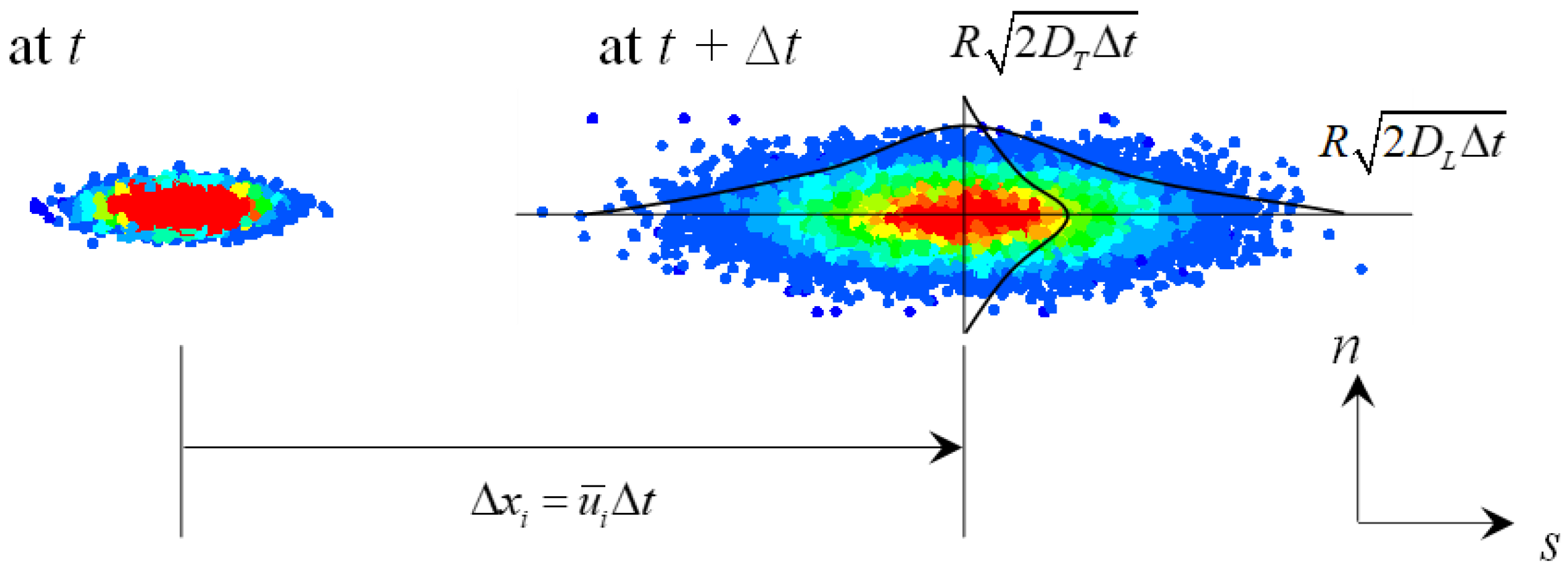
2.1. Particle Tracking Model (PTM)

The general particle tracking model is derived from the Itō stochastic differential equation as follow [33].

$$d{x}_i=A_{i}dt+B_{ij}d{W}_j$$

(5)

where $d{x}_i=x_i\left(t+\Delta t\right)-x_i\left(t\right)$ is displacement of a particle for $\Delta t$; $A_i$ is an arbitrary vector; $B_{ij}$ is an arbitrary tensor; and $d{W}_j=R\sqrt{\Delta t}$ is the Wiener process, which determines the random motion of particles using a random number, $R$. For a number of particles and infinitesimally small $\Delta t$, Equation (5) can be described using the Fokker–Plank equation, as shown in Equation (6) [27].

$$\frac{\partial p}{\partial t}+\frac{\partial }{\partial x_i}\left(A_{i}p\right)=\frac{{\partial }^2}{\partial x_i\partial x_j}\left(B_{ik}{B}_{jk}p\right)$$

(6)

where $p$ is the conditional probability density function. The Fokker–Plank equation mathematically coincides with the advection-dispersion equation as follows.

$$\frac{\partial \left(hC\right)}{\partial t}+\frac{\partial }{\partial x_i}\left({\overline{u}}_{i}hC\right)=\frac{\partial }{\partial x_i}\left[D_{ij}\frac{\partial \left(hC\right)}{\partial x_j}\right]$$

(7)

Therefore, $A_i$ and $B_{ij}$ in Equation (5) are defined using Equation (7), and Equation (5) can be rewritten as follows under the assumption, which has the coordinate system aligned with the flow direction.

$$x_i\left(t+\Delta t\right)=x_i\left(t\right)+{\overline{u}}_{i}dt+R\sqrt{2D_i\Delta t}$$

(8)

From Equation (8), displacement of a pollutant particle after $\Delta t$ is determined by both the deterministic and the random transports. The fourth-order Runge–Kutta scheme was adopted to solve the ordinary differential equation shown in Equation (8). In this study, the particle tracking model using Equation (8) is denoted as PTM. The aforementioned computation procedure was depicted in Figure 2. Pollutant cloud is transported by the depth-averaged velocity fields, and the scale of longitudinal (s) and transverse (n) direction mixing is determined by the computation of the random transport term.

In the 2D analysis, the deterministic displacement in Equation (8) is governed by the depth-averaged velocity fields calculated from the flow analysis model, Hydro Dynamic Model-2D (HDM-2D), which has been validated for several open channel flows [34]. The random transport term is controlled by the dispersion coefficient and the random number following the Gaussian distribution [35]. Generally, the dispersion coefficients are determined using empirical formulas. However, the empirical formulas have large bound of errors according to hydraulic conditions, which cause difficulties in determining the dispersion coefficients [36]. Thus, the dispersion coefficients were computed using the theoretical formula reported by Fischer et al. [5], as shown in Equations (9) and (10).

$$D_L=-\frac{1}{h}{\displaystyle {\int }_0^h{u^{\prime }}_s{\displaystyle {\int }_0^z\frac{1}{{\epsilon }_z}{\displaystyle {\int }_0^z{u^{\prime }}_s}}}dzdzdz$$

(9)

$$D_T=-\frac{1}{h}{\displaystyle {\int }_0^h{u^{\prime }}_n{\displaystyle {\int }_0^z\frac{1}{{\epsilon }_z}{\displaystyle {\int }_0^z{u^{\prime }}_n}}}dzdzdz$$

(10)

where ${u^{\prime }}_s=u_s-{\overline{u}}_s$ and ${u^{\prime }}_n=u_n-{\overline{u}}_n$ are the velocity deviations from the depth-averaged velocity in the longitudinal and transverse direction, respectively. In open channel flows, ${\epsilon }_z$ is known as the parabolic distribution over flow depth, as shown below [5].

$${\epsilon }_z=\kappa h{u}^{*}\left(\frac{z}{h}\right)\left(1-\frac{z}{h}\right)$$

(11)

where $\kappa$ is the von Karman constant. By incorporating Equations (9) and (10) into the advection-dispersion equation, previous research shows that simulation results of solute transport can display improved accuracy compared with the results using empirical formulas for dispersion coefficients [16,21].

The vertical velocity shears (${u^{\prime }}_n$, ${u^{\prime }}_s$) in Equations (9) and (10) were reproduced using the theoretical formulas and the depth-averaged flow fields from the simulation results by the HDM-2D. The theoretical formulas for $u_n$ and $u_s$ were demonstrated using the log profile [37] and the linear profile [38] as follows.

$$u_s\left(z\right)={\overline{u}}_s\left[1+\frac{\sqrt{g}}{\kappa C_h}\left(1+\ln \frac{z}{h}\right)\right]$$

(12)

$$u_n\left(z\right)={\overline{u}}_n+{\overline{u}}_s\left(\frac{2}{{\kappa }^2}+\frac{\sqrt{g}}{{\kappa }^3{C}_h}\right)\left(\frac{h}{r_c}\right)\left(\frac{z}{h}-\frac{1}{2}\right)$$

(13)

where $C_h$ is the Chezy coefficient and $r_c$ is the radius of curvature. Park et al. [21] reported that the velocity formulas shown in Equations (12) and (13) provide adequate computation results of the spatially varying dispersion coefficients in curved bends.

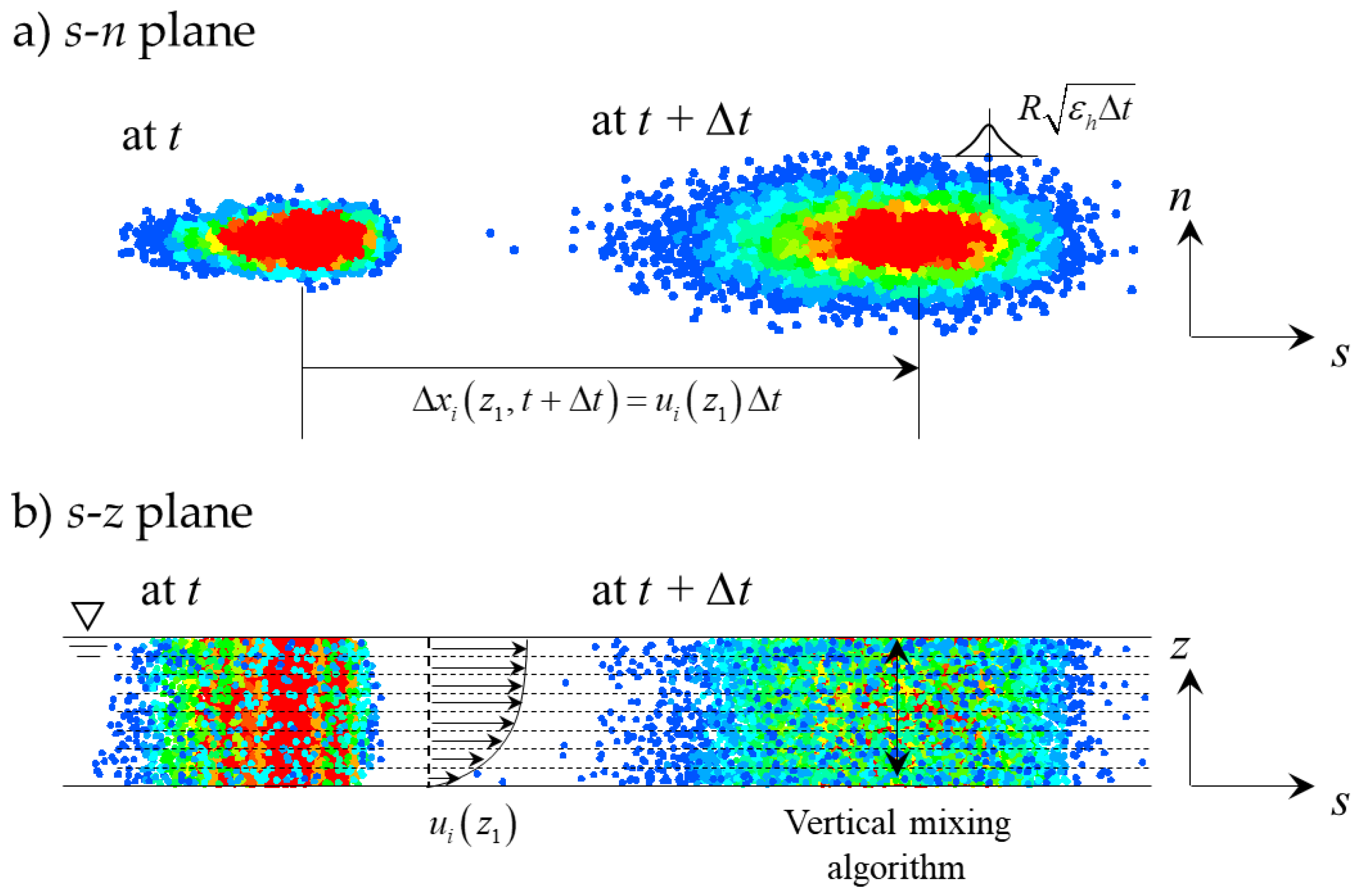
2.2. Particle Dispersion Model (PDM)

Fischer [39] modeled the shear dispersion in rivers into two sequential steps: the shear transport and the turbulent diffusion. Based on the study by Fischer [39], Park and Seo [31] developed the particle dispersion model (PDM), which computes the two-dimensional solute mixing using step-by-step computations of shear transport and vertical mixing. In the shear translation step, a particle position ($x_i$) after $\Delta t$ is determined using Equation (14).

$$x_i\left(z_1,t+\Delta t\right)=x\left(z_1,t\right)+u_i\left(z_1\right)\Delta t+R\sqrt{2{\epsilon }_h\Delta t}$$

(14)

where $z_1$ is the initial vertical position of a pollutant particle, ${\epsilon }_h=\alpha h{u}^{*}$ is the horizontal diffusion coefficient, and $\alpha$ is an empirical constant according to the hydraulic conditions. According to Equation (14), deterministic displacements of particles in longitudinal and transverse directions are determined by the vertical profiles of velocity.

After finishing the shear translation, the vertical position of pollutant particles belonging to the computational mesh are repositioned by the vertical mixing algorithm to finish the shear dispersion for $\Delta t$. The vertical mixing algorithm is given below.

$$x_i\left(z_2,t+\Delta t\right)=x\left(\frac{ah}{L},t+\Delta t\right)\mathrm{for}\beta n_p\left(x_i,t+\Delta t\right)$$

(15)

$$x_i\left(z_2,t+\Delta t\right)=x\left(z_1+R\sqrt{2{\epsilon }_z\Delta t},t+\Delta t\right)\mathrm{for}\left(1-\beta \right)n_p\left(x_i,t+\Delta t\right)$$

(16)

where $n_p$ is the number of particles in a computational mesh; $a$ is an integer from 1 to $L$; $L$ is the number of artificially divided vertical layer; $\beta =\Delta t/t_m$ when $\Delta t$ is shorter than $t_m$, otherwise $\beta =1$; and $t_m$ is the completion time for vertical mixing. The value of $\beta$ represents the degree of progress in complete vertical mixing. Thus, $\beta$% of entire particles within a computation mesh is evenly distributed across the artificially divided vertical layers using Equation (15), and the other particles are randomly rearranged by the turbulent diffusion shown in Equation (16). From the study of Fischer et al. [5] and Rutherford [10], $t_m$ can be defined as follows.

$$t_m=0.1\frac{h^2}{{\epsilon }_z}$$

(17)

From the aforementioned step-by-step computations, the PDM computes the two-dimensional solute transport, as described in Figure 3. According to this figure, solute particles are transported by vertical velocity shear and the random fluctuations in the s-n plane on each vertical layer. The velocity profiles were generated using Equations (12) and (13), which are used for computing the dispersion coefficients of the PTM. The transported particles were rearranged in a vertical layer by the vertical mixing algorithm using Equations (15) and (16). Figure 3b shows the particle distributions in the s-z plane after the vertical mixing is completed.

3. 2D Solute Mixing Simulation Results

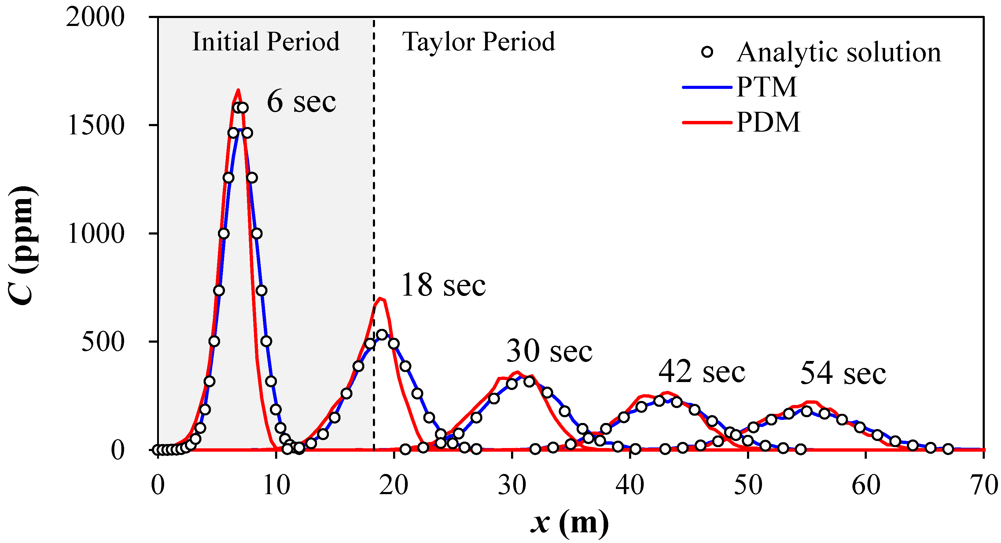
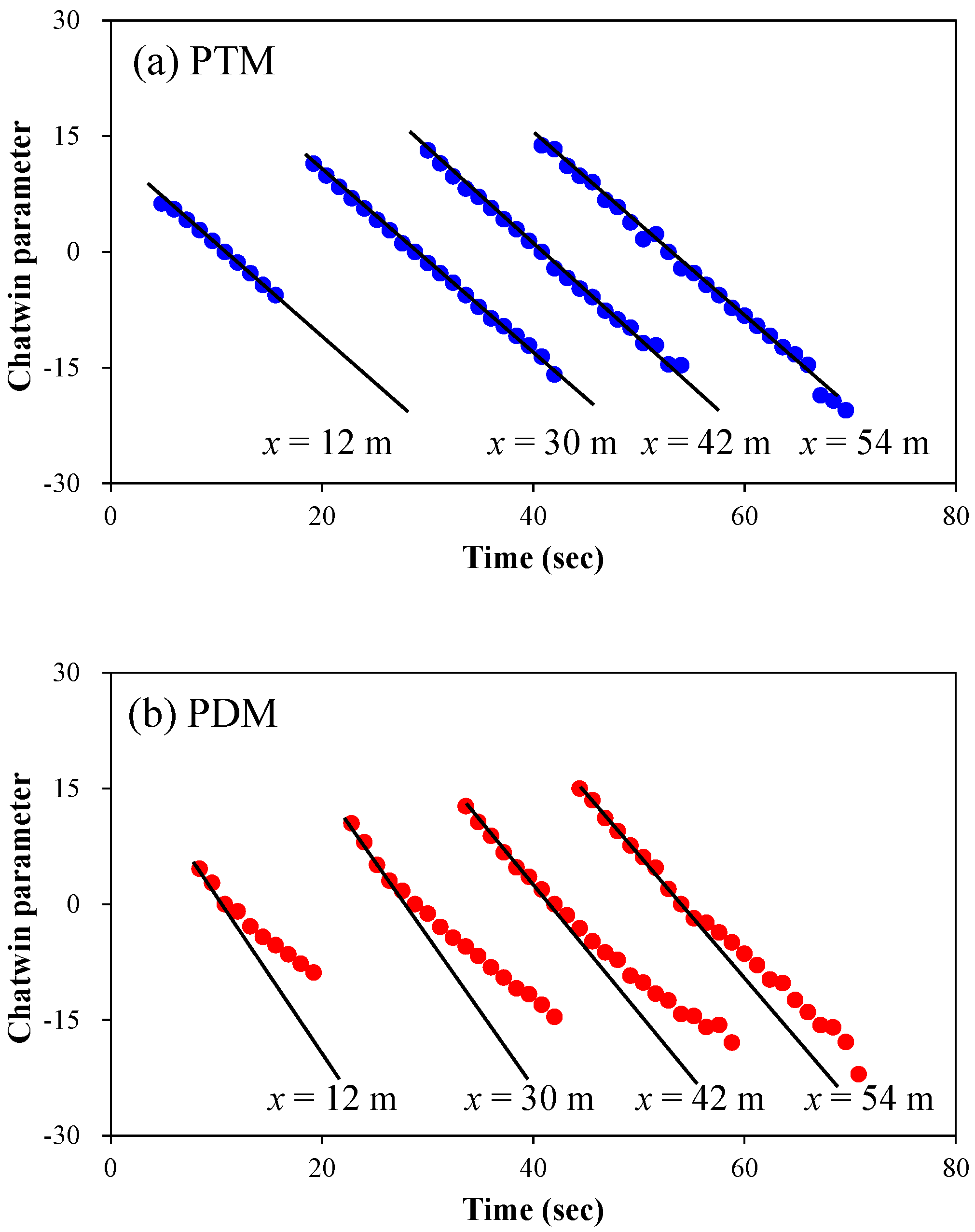
3.1. Model Validations

The simulation results of the two particle tracking models were validated by comparing with the analytic solution of the advection-dispersion equation. By assuming uniform flow in a straight channel with a rectangular cross section, the concentration of instantaneously introduced pollutant can be calculated using Equation (18).

$$C\left(s,n,t\right)=\frac{M/h}{4\pi t\sqrt{D_L{D}_T}}\left[\exp \left\{-\frac{{\left(s-s_0-{\overline{u}}_{s}t\right)}^2}{4D_{L}t}-\frac{{\left(n-n_0\right)}^2}{4D_{L}t}\right\}\right]$$

(18)

where $M$ is the total mass of pollutant (kg) and $\left(s_0,n_0\right)$ is the injection point. The longitudinal dispersion coefficient was inputted as $D_L=5.93h{u}^{*}$, which was derived by Elder [15], who assumed the log-profile for the longitudinal velocity shear. In the case of the transverse dispersion coefficient, $D_T=0.15h{u}^{*}$ was adopted following the study by Fischer et al. [5]. In this straight channel, the flow velocity is 1 m/s and the flow depth is 0.3 m. Particle tracking simulations were conducted under the aforementioned conditions by inputting 1 kg mass of pollutant using both the PTM and the PDM. The number of particles for particle tracking simulations was 30,000, and the concentration fields were calculated by counting the number of particles in a computational mesh as follows.

$$C\left(s,n,t\right)=\frac{m{n}_p\left(s,n,t\right)}{h\Delta A}$$

(19)

where $m=M/n_p$ is the mass of a particle (kg), $n_p$ is the number of particles in a computational grid, and $\Delta A=\Delta s\Delta n$ is a grid size (m²).

The concentration variations according to distance along the center of the channel are compared in Figure 4, where the range of the initial period was computed using Equation (2). The results by the PTM presented that the longitudinal dispersion was successfully reproduced by adopting Equations (9) and (12), instead of using $D_L=5.93h{u}^{*}$. Thus, the concentration curves of the PTM were well-fitted to the analytic solution in both the initial and the Taylor periods. On the other hand, the results by the PDM show skewed concentration curves in the initial period, and the results were gradually fitted to the analytic solution after t = 30 s, as reported by Park and Seo [31]. These results show the distinct differences between the two models, where the PTM derives the results by assuming a complete balance between the shear advection and the vertical diffusion, whereas the PDM directly calculates the process of achieving the balance.

The shape of the temporal variations of concentration curves of the PTM and the PDM were estimated using Chatwin’s parameter as follows [32,40,41].

$$\pm \sqrt{t\ln \left(\frac{C_{\max }\sqrt{t_{\max }}}{C\sqrt{t}}\right)}$$

(20)

where $t_{\max }$ is the time when the maximum concentration ($C_{\max }$) occurs. The parameter shown in Equation (20) makes a linear line when the results follow the Gaussian distribution according to the Fickian type dispersion. The calculation results of Chatwin’s parameter were plotted against time in Figure 5. The results of the PTM show clear linear lines in the entire computation domain. As the PTM is basically developed following Fick’s law, the results of the PTM show the symmetric concentation curves in the ideal straight channel. In case of the PDM, the values of Chatwin’s parameter obtained from the tail of the concentration curves deviated from the linear line made by the values calculated at the rising part of the concentration curve. After that, the deviations were gradually narrowed within the Taylor period. These results indicate that the concentration curves present tail and asymmetric curves in the initial period and they are gradually turned to symmetric curves even though there are no storage zones [31,39].

3.2. 2D Solute Mixing in the Meandering Channel

3.2.1. Temporal Variations of Concentration

The performance of two types of particle tracking model was evaluated by comparing with the tracer tests conducted in the meandering channel, showing the non-Fickian mixing properties [42]. The meandering channel has two bends with $r_c/W=2.5$ and the bends are connected with a straight part. The channel has a rectangular cross section of 1 m width and 15 m long. In this channel, the two-dimensional tracer tests were conducted using a salt solution. Here, 100,000 ppm of salt solution was instantaneously introduced as a vertical line source and the temporal changes of concentration were measured at 5 points on each of the 12 sections using conductivity sensors.

Table 1. Experimental and simulation conditions in the meandering channel.

Case	Q (m3/s)	h (m)	rc (m)	Manning’s nf	L	np
C306	0.06	0.3	85	0.013	300	30,000
C406	0.06	0.4	90	0.015	300	30,000

shows a summary of the experiment and the simulation conditions for flow and solute mixing analysis. The contour plot shown in Figure 6 is the velocity magnitude (U) distributions for Case C306 resulting from the HDM-2D. The velocity distributions show the increase of velocity in the inner bank of the channel bends, and the results were adequately reproduced flow in the channel bends compared with the measurements [42]. The particle tracking simulations were conducted using the results from the HDM-2D, and the vertical profiles of velocities were reproduced using Equations (12) and (13), known to adequately represent the shear flow in the meandering channel [21,31].

Figure 7 shows the particle tracking simulation results of Case C306 using the PTM and the PDM. The particle clouds of the PTM are more widely distributed in the longitudinal direction than those of the PDM. While the particle cloud crosses the first bend, the front of the particle cloud resulting from the PDM is transported to the inner bank of the bend, whereas the particles of the PTM are dispersed to the center of channel. It can also be seen in the second bend that the particle cloud of the PDM has a relatively shorter front compared with those of the PTM.

The temporal variations of concentration within the channel bends were plotted at y/W = 0.45, as shown in Figure 8. The value of concentration is normalized using the injection concentration ($C_0$). The main features of measured concentration curves are that the concentration curves have a steep, rising limb and long tail. These skewed concentration curves can be observed in the initial period [32] or the Taylor period, including a recirculation zone [43]. As the curvature of the meandering channel is not sharply curved enough to cause the recirculating flow [44], it can be said that the skewed concentration curves are not attributable to the storage effects. From Equation (2) and the hydraulic conditions shown in Table 1, the initial period was presumed to maintain for 144.3 s and 263.9 s in Case C306 and C406, respectively. Thus, the skewed concentration curves from the measurements were induced by the disproportion between the shear advection and the vertical diffusion. Even though the PTM adopts spatially varying dispersion coefficients to reproduce the mixing by the shear flow, the model shows the inherent limitations of the Fickian model. The results of the PTM presented nearly symmetric concentration distributions, of which the rising part shows large discrepancies from the measurements. On the other hand, the PDM properly reproduced the skewed concentration curves, which rapidly increase to the peak concentration and gradually decrease. These results seem to suggest that the tracer mixing is more adequately reproduced by the PDM than the PTM through direct computations of the shear dispersion process.

3.2.2. Statistical Properties of Concentration Curves in Channel Bends

The differences in the simulation results by the PTM and the PDM were scrutinized using Chatwin’s parameter and the statistical analysis. In Figure 9, the values of Chatwin’s parameter were plotted using the concentration curves shown in Figure 8. In Case C306, both models show discrepancies from the measurements on S4, but the results of the PDM properly followed the variations in the measurements on S9. Especially, the results of the PDM were adequately fitted to the measurements of Case C406. Overall, the PTM appears to have a moderate change in the values of Chatwin’s parameter compared with the measurements. These tendencies of the results from the PTM were also maintained in Case C406.

The time variation of Chatwin’s parameter indicates the temporal change of the concentration curves, in which the rising and falling parts of the concentration curves represent positive and negative values of Chatwin’s parameter, respectively. Thus, the slope of Chatwin’s parameter shown in Figure 9 is listed in

Table 2. Slope of the temporal variations of Chatwin’s parameters.

Case	Conc. Curve	1st Bend (S4 or S5)			2nd Bend (S9)
		Measurements [42]	PTM	PDM	Measurements [42]	PTM	PDM
C306	Rising part	−1.42	−0.72	−1.53	−1.28	−0.87	−1.30
	Falling part	−1.13	−0.71	−1.06	−0.68	−0.72	−1.13
C406	Rising part	−1.24	−0.92	−1.59	−1.60	−0.87	−1.74
	Falling part	−1.04	−0.90	−1.21	−0.81	−0.82	−0.78

by dividing into rising and falling parts. In general, the slope of the rising part is steeper than the falling part, as can be seen in Figure 8, and the values shown in Table 2 appear to support such variations. The lower values of the slope in the falling part than the rising part present that a concentration curve has a long tail. In the results by the PDM, these results can also be found, and the values of slope were overall similar to the measurements, except on S9 in Case C306. The results by the PTM maintained an almost constant slope in both the rising and falling parts of the concentration curves. Thus, the rising parts show large errors compared with the measurements.

The statistical properties of the concentration curves shown in Figure 8 are compared in

Table 3. Statistical properties of concentration curves in channel bends.

Case	Statistical Values	1st Bend (S4 or S5)			2nd Bend (S9)
		Measurements [42]	PTM	PDM	Measurements [42]	PTM	PDM
C306	$C_p/C_0$	0.045	0.035	0.034	0.013	0.011	0.012
	$t_p$ (s)	21.5	20.0	20.0	50.5	52.0	52.0
	${\mu }_t$ (s)	22.3	20.7	21.1	54.2	51.5	52.2
	${\sigma }_t^2$	6.4	12.0	8.9	35.5	28.8	21.4
	${\xi }_t$	0.74	0.34	0.71	0.52	0.18	0.55
C406	$C_p/C_0$	0.022	0.021	0.021	0.015	0.014	0.013
	$t_p$ (s)	36.5	38.0	38.0	65.3	66.0	65.0
	${\mu }_t$ (s)	37.1	38.6	38.3	68.2	66.9	69.3
	${\sigma }_t^2$	17.2	23.7	13.0	43.1	44.02	40.7
	${\xi }_t$	0.61	0.33	0.59	0.56	0.25	0.62

. The shape of the concentration curves can be defined using the peak concentration ($C_p$), time to the peak ($t_p$), time to centroid (${\mu }_t$), variance (${\sigma }_t^2$), and skewness (${\xi }_t$). The values of $C_p/C_0$, $t_p$, and ${\mu }_t$ show similar errors in both models compared with the measurements. The obvious differences between the two models can be found in the values of ${\sigma }_t^2$ and ${\xi }_t$. The PTM tends to overestimate the variance on the first bend of the channel, whereas it provides similar results in the second bend. In the case of the skewness, the PTM maintains low skewness values in both channel bends. As can be found in Table 2, the PTM calculates the concentration curves close to the Gaussian curve, and the skewed curve in the initial period is difficult to reproduce, even though the model adopts the dispersion coefficients including the effects of vertical velocity shear. Thus, the errors in the statistical characteristics of the PTM were reduced in the second bend, where the non-Fickian mixing properties within the initial period decreased. In case of the PDM, the statistical values indicate that the model properly reproduced the shape of the concentration curves, although the skewness in the second bend was slightly overestimated.

3.3. Model Applications in the Hongcheon River

The performance of the two particle tracking models within the Taylor period was evaluated by comparing them with the 2D tracer test results conducted in the Hongcheon River by Park and Seo [31]. The Hongcheon River is a tributary of the North Han River located in the Kangwon province of South Korea. The study site shows a mildly curved bend, as shown in Figure 10, and the tracer tests were executed under the hydraulic conditions given in

Table 4. Reach averaged hydraulic and simulation conditions in the Hongcheon River.

Q (m3/s)	h (m)	U (m/s)	rc (m)	Manning’s nf	L	np
2.15	0.91	0.05	148	0.036	200	20,000

. For the experimental conditions, the initial period would be maintained for 22.9 min according to Equation (2), and the Taylor period is estimated to occur 64 m from the tracer injection point when the averaged flow velocity (U) is considered. Thus, the results indicate that Section 1 and Section 2 in Figure 10 are included in the Taylor period.

The particle tracking simulations were conducted following the conditions listed in Table 4. The simulation results were plotted in Figure 11 with the temporal changes of concentration in Section 1 and Section 2. As reported by Park and Seo [31], the tracer cloud has an asymmetric shape owing to sidewall friction and irregular channel geometries even in the Taylor period. Thus, the concentration–time curves show a notably stretched tail of the falling part in Section 2, and these results were adequately reproduced using both models. These results revealed that the PTM is able to create the asymmetric concentration distribution that does not appear in the initial period. It can be inferred that the spatially varying dispersion coefficients computed by the vertical velocity profiles by Equations (9) and (10) are applicable to exhibit solute mixing in rivers including dead zones. The main difference between the two simulation results is that the rising part of the concentration curves by the PDM increases sharply compared with the results by the PTM.

The statistical properties of the concentration–time curves were compared in

Table 5. Statistical properties of concentration curves in the Hongcheon River.

Statistical Values	Sec. 1 (y/W = 0.30)			Sec. 2 (y/W = 0.25)
	Measurements [31]	PTM	PDM	Measurements [31]	PTM	PDM
$C_p$ (ppb)	25.4	23.3	28.6	2.50	1.9	3.0
$t_p$ (min)	36.4	40.0	41.0	127.0	131.0	123.0
${\mu }_t$ (min)	39.2	41.6	42.5	138.5	146.5	147.9
${\xi }_t$	0.66	0.56	0.70	1.06	0.82	1.02

. Both models show similar values in $C_p$, $t_p$, and ${\mu }_t$ compared with the measurements. These results explain that both simulation results present appropriate solute mixing in the intermediate mixing region, where the influence of the initial period is negligible. The featured differences can be found in the value of ${\xi }_t$, where the percentage error of the PTM was in the range of 14.9–22.6% and the PDM was in the range of 1.9–6.1%. From the results, the PDM is reaffirmed to be predominant for the non-Fickian mixing simulations compared with the PTM.

4. Discussion

The performance of two particle tracking models was evaluated by comparing the analytic solution and the 2D tracer test results. The results consistently show that the PDM is more adaptable to reproduce non-Fickian mixing in the initial period. On the other hand, the results by the PTM were inappropriate to demonstrate the skewed concentration curves during the initial mixing process. These results revealed the inherent limitations of the Fickian model, which was derived under the assumption of equilibrium between the shear and diffusion processes [4]. Because the initially skewed concentration distributions originated from the velocity shear [11,39], the PDM included the effects of vertical velocity shear into the computation algorithm, as shown in Figure 3. In the case of the PTM, the model is based on the Fickian model and the shear effects were incorporated into the dispersion coefficients. Thus, the PTM shows discrepancies against the measurements in the initial period, even though the dispersion coefficients computed using the vertical velocity profiles were reported to improve the accuracy of the simulation results compared with empirical formulas [6,16,21].

The non-Fickian mixing behavior is also known to occur by breaking the equilibrium state in the Taylor period because of the complex channel geometries [28,30,31,40]. Thus, to exhibit skewed concentration distributions by the channel irregularities, previous studies adopted dead zone models [29,45] or statistical models [46] for one-dimensional mixing problems. However, these approaches have not been expanded to 2D mixing problems. The PTM computes the 2D shear dispersion using the spatially varying dispersion coefficients. From the application of the dispersion coefficients that change according to the velocity structures [21], the PTM reproduced the long tail of concentration curves induced by the channel geometries in the application results of the Hongcheon River. The results, however, were insufficient to reproduce the steep rising part of the concentration curves. An alternative approach has been reported, which employed vertical velocity formulas for the computation of the deterministic transport of each particle, instead of the Fickian approach [24,31]. The aforementioned direct computation method for shear flow dispersion was employed for the PDM, and the model successfully presented the skewed concentration curves due to the irregular channel geometries.

5. Conclusions

In this study, two particle tracking models incorporating the effects of vertical velocity shear were compared using the spatial and temporal variations of concentration curves. The PTM is developed based on Fick’s law, in which the dispersion coefficients are employed to compute the longitudinal and transverse dispersion. The dispersion coefficients in the PTM were calculated using the triple integration of velocity deviations suggested by the study of Fischer et al. [5]. The other model denoted as PDM applied step-by-step computation algorithms to reproduce the shear flow dispersion instead of adopting Fick’s law. The model also adopted the vertical profiles of velocity to compute the shear translation of particles placed on each vertical layer. The main difference of these two models is that the PTM is applicable only within the Taylor period, where Fick’s law is valid, whereas the PDM can be used in both the initial and Taylor periods. Thus, to test the applicability of the two models, the models were applied to the test cases of the ideal straight channel and the meandering channel and the shape of the concentration curves was compared.

In the ideal straight channel case, the simulation results by the two models were validated by comparing with the analytic solution of the advection-dispersion equation. The concentration–distance curves of the PTM successfully reproduced the analytic solutions in the entire test domain. However, the PDM shows large discrepancies in the initial period compared with the analytic solution, and the differences were gradually reduced in the Taylor period. The analytic solution and the PTM produced symmetric concentration curves even in the initial period, whereas the results by the PDM show a skewed shape. These differences were distinctively found from the temporal variations of Chatwin’s parameter, in which the PTM follows the linear line and the PDM shows deviations from the linear line in the falling part of the concentration curve. The deviations in the results of the PDM were gradually reduced to become a linear line, which indicates the symmetric concentration curve. Thus, the PDM properly reproduced the procedures of the balance between the shear advection and the vertical diffusion, which are not observed in the Fickian model.

Solute mixing simulations were conducted in the meandering channel, which shows asymmetric concentration curves due to the non-Fickian mixing features. The performance of the two models were investigated by comparing Chatwin’s parameter and the statistical properties. The results by the PTM show the symmetric distribution, in which the slope of Chatwin’s parameter was nearly constant and the skewness was maintained at a low value. On the other hand, the PDM presented a long tail of the concentration curves in the channel bends, and the skewness decreased in the second bend compared with the first bend, as observed from the measurements. The performance of the PDM was reaffirmed from the application results in the Hongcheon River. Even though the PTM adequately reproduced the skewed concentration curves because of the channel irregularities, the PDM more accurately demonstrated the asymmetric variations of concentration. These results reveal that the direct computation algorithm of the shear dispersion provides more accurate results than the model following Fick’s law.

References

1. Piasecki, M.; Katopodes, N.D. Identification of stream dispersion coefficients by adjoint sensitivity method. J. Hydraul. Eng. 1999, 125, 714–724. [Google Scholar] [CrossRef]
2. Seo, I.W.; Lee, M.E.; Baek, K.O. 2D modeling of heterogeneous dispersion in meandering channels. J. Hydraul. Eng. 2008, 134, 196–204. [Google Scholar] [CrossRef]
3. Albers, C.; Steffler, P. Estimating transverse mixing in open channels due to secondary current-induced shear dispersion. J. Hydraul. Eng. 2007, 133, 186–196. [Google Scholar] [CrossRef]
4. Taylor, G.I. The dispersion of matter in turbulent flow through a pipe. Proc. R. Soc. Lond. A Math. Phys. Eng. Sci. 1954, 223, 446–468. [Google Scholar]
5. Fischer, H.B.; List, J.E.; Koh, R.C.Y.; Imberger, J.; Brooks, N.H. Mixing in Inland and Coastal Waters, 2nd ed.; Academic Press: San Diego, CA, USA, 1979; pp. 100–107. [Google Scholar]
6. Lee, M.E.; Seo, I.W. 2D finite element pollutant transport model for accidental mass release in rivers. KSCE J. Civ. Eng. 2010, 14, 77–86. [Google Scholar] [CrossRef]
7. Pilechi, A.; Mohammadian, A.; Rennie, C.D.; Zhu, D.Z. Efficient method for coupling field data and numerical modeling for the estimation of transverse mixing coefficients in meandering rivers. J. Hydraul. Eng. 2016, 142, 04016009. [Google Scholar] [CrossRef]
8. Park, I.; Song, C.G. Analysis of two-dimensional flow and pollutant transport induced by tidal currents in the Han River. J. Hydroinf. 2018, 20, 551–563. [Google Scholar] [CrossRef]
9. Lau, Y.L.; Krishnappan, B.G. Transverse dispersion in rectangular channels. J. Hydraul. Div. 1977, 103, 1173–1189. [Google Scholar]
10. Rutherford, J.C. River Mixing; John Wiley and Sons: London, UK, 1994; pp. 62–63. [Google Scholar]
11. Boxall, J.B.; Guymer, I. Analysis and prediction of transverse mixing coefficients in natural channels. J. Hydraul. Eng. 2003, 129, 129–139. [Google Scholar] [CrossRef]
12. Zhang, W.; Zhu, D.Z. Transverse mixing in an unregulated Northern River. J. Hydraul. Eng. 2011, 137, 1426–1440. [Google Scholar] [CrossRef]
13. Baek, K.O.; Seo, I.W. Empirical equation for transverse dispersion coefficient based on theoretical background in river bends. Environ. Fluid Mech. 2013, 13, 465–477. [Google Scholar] [CrossRef]
14. Seo, I.W.; Baek, K.O.; Jeon, T.M. Analysis of transverse mixing in natural streams under slug tests. J. Hydraul. Res. 2006, 44, 350–362. [Google Scholar] [CrossRef]
15. Elder, J.W. The dispersion of marked fluid in turbulent shear flow. J. Fluid Mech. 1959, 5, 544–560. [Google Scholar] [CrossRef]
16. Lee, M.E.; Seo, I.W. Analysis of pollutant transport in the Han River with tidal current using a 2D finite element model. J. Hydro Environ. Res. 2007, 1, 30–42. [Google Scholar] [CrossRef]
17. Baek, K.O.; Seo, I.W.; Jung, S.J. Evaluation of dispersion coefficients in meandering channels from transient tracer tests. J. Hydraul. Eng. 2006, 132, 1021–1032. [Google Scholar] [CrossRef]
18. Seo, I.W.; Choi, H.J.; Kim, Y.D.; Han, E.J. Analysis of two-dimensional mixing in natural streams based on transient tracer tests. J. Hydraul. Eng. 2016, 142, 04016020. [Google Scholar] [CrossRef]
19. Shin, J.; Seo, I.W.; Baek, D. Longitudinal and transverse dispersion coefficients of 2D contaminant transport model for mixing analysis in open channels. J. Hydrol. 2020, 583, 124302. [Google Scholar] [CrossRef]
20. Kim, D. Assessment of longitudinal dispersion coefficients using Acoustic Doppler Current Profilers in large river. J. Hydro Environ. Res. 2012, 6, 29–39. [Google Scholar] [CrossRef]
21. Park, I.; Seo, I.W.; Shin, J.; Song, C.G. Experimental and numerical investigations of spatially-varying dispersion tensors based on vertical velocity profile and depth-averaged flow field. Adv. Water Resour. 2020, 142, 103606. [Google Scholar] [CrossRef]
22. Wong, K.T.M.; Lee, J.H.W.; Choi, K.W. A deterministic Lagrangian particle separation-based method for advective-diffusion problems. Commun. Nonlinear. Sci. 2008, 13, 2071–2090. [Google Scholar] [CrossRef]
23. Dimou, K.N.; Adams, E.E. A random-walk, particle tracking model for well-mixed estuaries and coastal waters. Estuar. Coast. Shelf Sci. 1993, 37, 99–110. [Google Scholar] [CrossRef]
24. Weitbrecht, V.; Uijttewaal, W.; Jirka, G.H. 2-D particle tracking to determine transport characteristics on shallow flows. In Proceedings of the International Symposium on Shallow Flows (IAHR), Delft, The Netherlands, 6–8 September 2004. [Google Scholar]
25. Gomez-Gesteira, M.; Montero, P.; Prego, R.; Taboada, J.J.; Leitao, P.; Ruiz-Villarreal, M.; Neves, R.; Perez-Villar, V. A two-dimensional particle tracking model for pollution dispersion in A Coruna and Vigo Rias (NW Spain). Oceanol. Acta 1999, 22, 167–177. [Google Scholar] [CrossRef] [Green Version]
26. Suh, S.W. A hybrid approach to particle tracking and Eulerian-Lagrangian models in the simulation of coastal dispersion. Environ. Model. Softw. 2006, 21, 234–242. [Google Scholar] [CrossRef]
27. Tomson, A.F.B.; Gelhar, L.W. Numerical simulation of solute transport in three-dimensional, randomly heterogeneous porous media. Water Resour. Res. 1990, 26, 2541–2562. [Google Scholar]
28. Day, T.J. Longitudinal dispersion in natural channels. Water Resour. Res. 1975, 11, 909–918. [Google Scholar] [CrossRef]
29. Czernuszenko, W.; Rowiński, P.M.; Sukhodolov, A. Experimental and numerical validation of the dead-zone model for longitudinal dispersion in rivers. J. Hydraul. Res. 1998, 36, 269–280. [Google Scholar] [CrossRef]
30. Mazijk, A.; Veling, E.J.M. Tracer experiments in the Rhine Basin: Evaluation of the skewness of observed concentration distributions. J. Hydrol. 2005, 307, 60–78. [Google Scholar] [CrossRef]
31. Park, I.; Seo, I.W. Modeling non-Fickian pollutant mixing in open channel flows using two-dimensional particle dispersion model. Adv. Water Resour. 2018, 111, 105–120. [Google Scholar] [CrossRef]
32. Chatwin, P.C. On the interpretation of some longitudinal dispersion experiments. J. Fluid Mech. 1971, 48, 689–702. [Google Scholar] [CrossRef]
33. Itō, K.; Nisio, M. On stationary solutions of a stochastic differential equation. J. Math. Kyoto Univ. 1964, 4, 1–75. [Google Scholar] [CrossRef]
34. Song, C.G.; Seo, I.W.; Kim, Y.D. Analysis of secondary current effect in the modeling of shallow flow in open channels. Adv. Water Res. 2012, 41, 29–48. [Google Scholar] [CrossRef]
35. Box, G.E.P.; Muller, M.E. A note on the generation of random normal deviates. Ann. Math. Stat. 1958, 29, 610–611. [Google Scholar] [CrossRef]
36. Wang, Y.; Huai, W. Estimating the longitudinal dispersion coefficient in straight natural rivers. J. Hydraul. Eng. 2016, 142, 04016048. [Google Scholar] [CrossRef]
37. Rozovskii, I.L. Flow of Water in Bends of Open Channels; Academy of Science of Ukrainian SSR: Moscow, Russia, 1957. [Google Scholar]
38. Odgaard, A.J. Meander flow model. I: Development. J. Hydraul. Eng. 1986, 112, 1117–1136. [Google Scholar] [CrossRef]
39. Fischer, H.B. Methods for Predicting Dispersion Coefficients in Natural Streams, with Applications to Lower Reaches of the Green and Duwamish Rivers Washington; US Government Printing Office: Washington, DC, USA, 1968; pp. A22–A25.
40. Guymer, I. Longitudinal dispersion in sinuous channel with changes in shape. J. Hydraul. Eng. 1998, 124, 33–40. [Google Scholar] [CrossRef]
41. Marion, A.; Zaramella, M. Effects of velocity gradients and secondary flow on the dispersion of solutes in a meandering channel. J. Hydraul. Eng. 2006, 132, 1295–1302. [Google Scholar] [CrossRef]
42. Seo, I.W.; Park, S.W. Effect of velocity structures on tracer mixing in a meandering channel. J. Korean Soc. Civil. Eng. 2009, 29, 35–45. [Google Scholar]
43. Kim, J.S.; Baek, D.; Park, I. Evaluating the impact of turbulence closure models on solute transport simulations in meandering open channels. Appl. Sci. 2020, 10, 2769. [Google Scholar] [CrossRef]
44. Hickin, E.J. Mean flow structure in meanders of the Squamish River, British Columbia. Can. J. Earth Sci. 1978, 15, 1833–1849. [Google Scholar] [CrossRef] [Green Version]
45. Schmid, B.H. On the transient storage equations for longitudinal solute transport in open channels: Temporal moments accounting for the effects of first-order decay. J. Hydraul. Res. 1995, 33, 595–610. [Google Scholar] [CrossRef]
46. Chatwin, P.C. Presentation of longitudinal dispersion data. J. Hydraul. Div. 1980, 106, 71–83. [Google Scholar]
Figure 1. Descriptions of solute mixing by shear flow in initial and Taylor periods.
Water 12 03535 g001
Figure 2. Conceptual diagrams of the computation procedures in the particle tracking model (PTM).
Water 12 03535 g002
Figure 3. Descriptions of the two-dimensional particle mixing procedures using the particle dispersion model (PDM).
Water 12 03535 g003
Figure 4. Comparisons of concentration–distance curves of the PTM and the PDM in the straight channel.
Water 12 03535 g004
Figure 5. Time evolution of Chatwin’s parameter for Ct curves at the center of the channel.
Water 12 03535 g005
Figure 6. Descriptions of the meandering channel and the velocity magnitude resulting from the HDM-2D (C306).
Water 12 03535 g006
Figure 7. Particle transport simulation results using the two types of particle tracking models (C306).
Water 12 03535 g007
Figure 8. Temporal variations of concentration curves at y/W = 0.45 within the channel bends.
Water 12 03535 g008
Figure 9. Comparisons of Chatwin’s parameter of Ct curves obtained in the channel bends.
Water 12 03535 g009
Figure 10. Outlines of the study site and the velocity distributions in the Hongcheon River.
Water 12 03535 g010
Figure 11. Comparisons of temporal concentration variations in the Hongcheon River.
Water 12 03535 g011