Impact of Climate Change on Soil Erosion in the Lam Phra Phloeng Watershed

Abstract

Soil erosion plays a vital role in reducing reservoir capacity. The Lam Phra Phloeng (LPP) dams were built for flood protection and irrigation. However, they have experienced reservoir sedimentation, and the capacity of the reservoir has decreased. The surrounding soil surface was easily eroded and transported by heavy rainfall and surface runoff to streams and eventually into the reservoir. Understanding this soil erosion and sedimentation is necessary for preventing further decline of reservoir capacity and water management. This research aims to estimate long-term average annual soil erosion and predict sediment yield in the reservoir due to climate change. The methodology is determined soil loss parameters and sediment yield using the Universal Soil Loss Equation (USLE) with the Sediment Delivery Ratio (SDR). The USLE and SDR methods differed from field data, with an average absolute error of 4.0%. The Global Climatic Model, Institute Pierre Simon Laplace-Climate Model version 5A (IPSL-CM5A-MR), with Representative Concentration Pathways (RCP) 2.6, 4.5, and 8.5, was downscaled and analyzed to forecast future rainfall in the watershed. The high intensity of rainfall contributed to higher soil erosion, in RCP 8.5. Interestingly, the high and very high-risk areas increased, but the moderate risk area declined, indicating that the moderate risk area should be a priority in land management. However, the heavy rainfall and high slope gradient led to a slight increase in the soil erosion in some areas because the land covers were evergreen and deciduous forest. The prediction of sediment yield was positively correlated with the intensity of rainfall in the central part of the watershed, because the rainfall and runoff led the sediment to the river and streams, indicating that the land cover should be managed to prevent capacity decline.

1. Introduction

Nowadays global disasters are being caused by human activity and climate change [1,2]. One problem is soil erosion, affecting the ecosystem, public utility system, and agricultural productivity [3]. Several factors affect soil erosion, such as water, ice (glacier), snow, air (wind), plants, animals, and human action [4].

Generally, a soil erodes slowly over most areas, but it erodes significantly in areas with heavy rainfall, high slope, intensive agriculture, deforestation, and urban sprawl. Soil erosion causes sediments to advect to rivers or streams, which leads to dead storage. Sedimentation increases the load on dams and decreases the useful storage capacity of reservoirs. Soil loss in the watershed of the Shihmen Reservoir, Taiwan, was over 9700 t/km²/year [5,6]. Nguyen and Chen [7] showed that the Shihmen River was subject to a sediment delivery ratio of approximately 0.48. Similarly, the total soil loss in Europe was estimated at 970 million t/year [8]. Ricci et al. evaluated the soil loss in Southeast Italy and found that the channel flow had the highest deposition, due to the alluvium in the central plain [9]. Yang et al., considered the relation between the erosion and deposition upstream of the Yellow River, using least-squares regression and partial least squares regression and fitted an accurate model [10]. In the 1990s, a rapid increase in human development caused significant environmental problems, for example deforestation and slope mass movement, in many areas of Thailand. The Thai Land Development Department (LDD) studied regional soil erosion in Thailand and acquired data for every region of Thailand [11]. Additionally, the LDD published a soil loss map of Thailand in 2002 showing that the soil loss of the Lam Phra Phloeng (LPP) (14.50561° N, 101.78058° E) watershed depended on the slope gradient and land cover. With a high gradient (≥35%) and forestation, the soil erosion was 0–1250 t/km²/year. The evergreen and deciduous forests led to a reduced soil erosion rate. A low gradient (<35%) and deforestation led to a soil erosion rate of 1250–3125 t/km²/year, because field crops and farms could not protect the soil from erosion. Significantly, a flat gradient and urban sprawl led to an erosion rate of 3125 t/km²/year, because there were no evergreens or forest to reduce soil erosion [11].

The Universal Soil Loss Equation (USLE) was designed to assess long-term average annual soil loss from field slopes under specific land use and management [12]. There are many models, for example the Soil & Water Assessment Tool (SWAT) and Variable Infiltration Capacity (VIC), that perform well in determining runoff and soil loss [13]. SWAT is based on widely accepted algorithms for modelling hydrological processes. It is suitable for evaluating different land use scenarios, with a fine spatial resolution, and allows for a higher temporal resolution of outputs. However, this is useful, only when sufficient time is available, due to the high application effort required, and adequate input data is available [14]. VIC is preferred for predicting soil loss on a regional scale, so the coarse-grid scale, that it uses, should be considered, when analysis on a local scale is need. There are several limitations to long-term predictions derived from gridded meteorology. Alewell et al. showed that process-based physical models, compared with simpler structured empirical models, for example USLE algorithms, led to similar results [15]. In addition, USLE together with the Geographic Information System (GIS), has been widely applied to analyze soil erosion. Thinley applied a spatial modeling technique and USLE to evaluate soil erosion in the upper part of the LPP area between 2000 and 2008 [16]. The high rate of soil loss was associated with the intensity of rainfall. The average annual sediment yield was increased from 12,030 to 12,840 t/km²/year. However, the precision of soil loss estimation factors, using USLE depended on the accuracy of input factors (i.e., rainfall-runoff erosivity, soil erodibility, slope length, slope steepness, vegetation cover, and conservation practice). If regional soil erosion is augmented with local factors, it will yield higher precision [16].

The Sediment Delivery Ratio (SDR) is a sediment yield evaluation method that defines the sediment yield from an area by the gross erosion of the same area. Selly found that sediment in a reservoir decreased the capacity and increased the load on the dam wall. Sediment in a canal caused flooding, as the canal was shallower [17]. Also, the sediment may induce a chemical reaction with the dam and erode its concrete structure [18]. Sediment yield and SDR are thus necessary to evaluate water management and protect dams.

The Lam Phra Phloeng (LPP) dam is located in the central part of Thailand (14.50561° N, 101.78058° E). It has been used for agriculture and flood protection in the northeastern part of Nakhon Ratchasima since 1967 [19]. Most of the area in the upstream watershed has been deforested to cultivate sugarcane and cassava. After the crop has been harvested, the land is tilled and becomes sensitive to sheet erosion [20]. Due to the steep slope near the boundary of the watershed and the deforestation from agriculture and urbanization, the watershed is now facing serious soil erosion. Therefore, evaluation of the erosion and sediment yield in the LPP reservoir is necessary.

Although several researchers have focused on soil erosion in the watershed, few have taken a step further and calculated the sediment delivery to the bed of the reservoir, specifically, under global climate change conditions. This study applied the USLE and SDR models to fill this gap. The objective is to predict long-term soil erosion and predict sediment yield in the reservoir, due to climate change, to improve the declining capacity of the reservoir and water planning and management. A Global Climate Model (GCM), Institute Pierre Simon Laplace-Climate Model version 5A (IPSL-CM5A-MR) from Coupled Model Intercomparison Project-5 (CMIP5) and three scenarios, i.e., RCP 2.6, RCP 4.5, and RCP 8.5, in the LPP watershed, were used to predict future rainfall data via Sananmuang’s method [21], from the correlation between rainfall and water surface in the central part of Thailand [22,23]. Field measurements and other methods were used to validate the USLE and SDR results. Future rainfall was assigned as a rainfall-runoff erosivity factor to estimate the soil erosion using the USLE and SDR methods in the LPP reservoir.

2. Study Area

2.1. General and Topography

Using the 30 × 30 m Digital Elevation Model (DEM) built by the LDD [11], Figure 1 illustrates the LPP watershed in Nakhon Ratchasima, Northeastern Thailand. The ground elevations are 233–1309 m above mean sea level. The watershed covers 815.2 km². Approximately 52% of the watershed area is part of the Khao Yai National Park (the first national park of Thailand that UNESCO declared a world heritage site on 14 July 2005). The upstream watershed borders the national park, which contains a mountain and deciduous forest. Rainfall is typically low, but is excessive in the rainy season, causing annual flooding. In 1967, the Thai Royal Irrigation Department (RID) operated the LPP dam, with a retention capacity of 170 million m³, to prevent floods in the rainy seasons and for irrigation in the dry seasons. This watershed has a major river, the Lam Phra Phloeng River, so sediment is eroded and moved into the LPP reservoir.

2.2. Rainfall-Runoff

Normally, the climate of the LPP watershed is tropical. It is affected by the Southwest Asia Monsoon and typhoons in the rainy season and by the Northeast Asia Monsoon in the winter. This area has three seasons: the rainy season from June to October, the winter from November to January, and the summer from February to May. Nine meteorological stations were available: Nong Sai Tai, Nong Chok, Sub Sai Thong, M.145, Huai Krok De, Khlong Pla Kang, Tar Nam Sub, Ban Bu Tako, and Din Udom. The mean annual rainfall was 1174 mm [24]. Most rainfall is in the upstream watershed, between 1300 and 1350 mm/year (Figure 2a). The High soil erosion is caused by the heavy rainfall and steep slopes.

2.3. Soil Groups

The 1:25,000 scale maps, drawn by the LDD [11], show that the soil fell into 12 groups, and some uncharacterized areas, i.e., cliffs, forest, land reserves, urban areas, and water bodies (Figure 2b). The soil groups are listed in

Table 1. Soil erodibility factors (K_m) in the LPP watershed, taken from LDD [11].

Soil Group Index	Distinct Characteristics	Km
22	Very deep coarse loam soil group arisen from the coarse sand distributary sediment	0.05
29	Deep to very deep clay soil group arisen from the fine mass parent material	0.25
31	Deep to very deep clay soil group arisen from the fine mass parent material, found in a mountainous area	0.25
35	Deep to very deep fine loam soil group arisen from distributary sediment or coarse mass parent material	0.24
37	Moderate deep coarse loam soil group arisen from material degradation or coarse alluvium to accumulate on top of the rockfall stratum at a 50–100 cm depth from the ground surface	0.24
40	Deep to very deep coarse loam soil group arisen from distributary sediment or coarse parent material	0.24
44	Thick sand soil group arisen from distributary sediment or coarse grain sediment	0.04
47	Shallow soil group to a rock wall layer	0.29
48	Shallow soil group to laterite or band iron formation on top of a clay layer	0.24
52	Shallow soil group to a marl or lime layer	0.25
55	Moderate deep soil group to a rock wall, rock waste, rocks, or laterite	0.25
56	Moderate deep soil group to a rock wall, rock waste, or laterite	0.24

. Soil group labelled 47 covered the largest area, 43.4% of total area. Most of the topsoil was shallow rock with rubble, so it was not fertile. However, some areas could not be surveyed because they were cliffs, forests or land reserve areas.

2.4. Slope Gradient

The 30 × 30 m Digital Elevation Model (DEM) by the LDD [11] (Figure 2c) showed that the landscape of the LPP watershed was both flat and mountainous. The slopes were generally small in the center of the watershed, covering 32%. However, the boundary is steep, covering 21% of the area.

2.5. Land Cover and Erosion-Protected Area

The LDD [11] divided the land cover into 13 types, using 1:25,000 scale map data (Figure 2d). The map showed that most areas were field crops (39.8%) and evergreen forest (26.8%). The planted areas protected the topsoil from soil erosion. Although Ashraf et al. [25] studied the influence of land cover on sediment and showed that human activities strongly affected the runoff, we considered the land cover as unchanged, because the LDD map was only one available and change in the national park area was severely constrained by legislation.

3. Methodology

Data flow in our study is shown in Figure 3. The data were collected from field investigations and from the Thai RID, LDD and Water Resources Department. The data was analyzed using the USLE and SDR models and validated with our field data. The scenarios of the GCM were applied using the Institute Pierre Simon Laplace-Climate Model version 5A (IPSL-CM5A-MR), augmented with the Representative Concentration Pathways (RCP), 2.6, 4.5 and 8.5, to evaluate climate change in the LPP watershed. This model was selected, because the scenarios offered the minimum bias and root mean square error on annual precipitation [22]. RCP 2.6 and 8.5 represent the most severe climate changes, and RCP 4.5 was the most likely event [23]. Soil erosion and sediment yield, due to climate change, were then predicted using the USLE and SDR models.

3.1. Universal Soil Loss Equation (USLE)

The USLE is an equation representing the potential long-term average annual soil loss. The equation predicts the long-term rate of erosion on a field slope based on rainfall pattern, soil type, topography, vegetation, and management practice [12]. The USLE has been applied to analyze soil erosion at different scales in previous research. The USLE predicts $A_m$, the long-term average annual rate of soil loss (t/km²/year) [26]:

$$A_m=R_m\times K_m\times L\times S\times C\times P$$

(1)

where $R_m$ is the rainfall factor (10⁶ joule-mm/km²/hr/year), $K_m$ is the soil erodibility (t-hour/10⁶ joule/mm), $L$ is the slope length, $S$ is the slope steepness, $C$ is vegetation cover, and $P$ is conservation practice.

The USLE has the following advantages: (i) it is efficient, since the parameters are separated into layers; and (ii) the soil erosion in each position can be digitized on a small scale and compared with field data at the same position. However, the precision of the USLE depends on soil type, slope gradient, and slope length. The soil type should be in the medium texture region, the slope gradient in the range of 3–18%, and the slope length <400 m. The USLE can provide only the long-term average soil erosion. In the LPP watershed, the soil types were rock, loam and sand, i.e., medium soil types. Most slope gradients were in the range of 1–20%, and slope lengths were lower than 330 m.

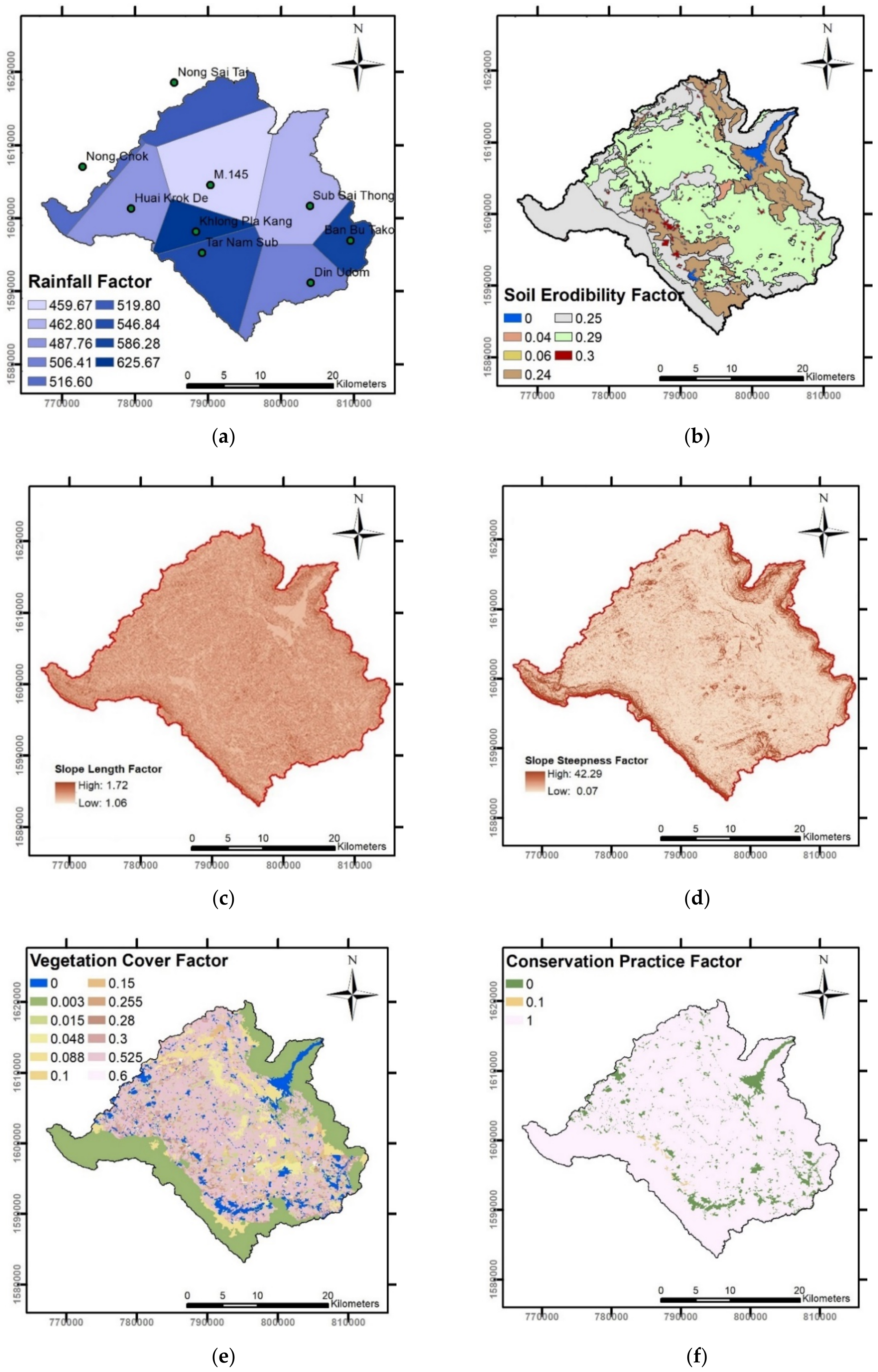
3.1.1. Rainfall Factor (R_m)

The rainfall factor, R_m, is calculated from [11]:

$$R_m = 0.4669X – 12.1415$$

(2)

where $X$ is the average rainfall (mm/year). The average annual rainfall values of the LPP watershed from 2005 to 2015 rainfall data were digitized using the Thiessen polygon method (Figure 4a). The Thiessen polygon method was selected because it is optimal for a small area. R_m is significant because the soil erosion was affected by future rainfall.

3.1.2. Soil Erodibility Factor (K_m)

The soil erodibility (K_m) was based on the 1:25,000 soil group map [11]—see Figure 4b and Table 1. K_m in the LPP watershed ranged from sandy loam (0.04) to rock (0.25). The coarse-grained soil led to low K_m, because the sediment transport depended on the size of the material. Although the soils were eroded, they did not move toward the river. The fine-grained soil contributed to high K_m, due to the low mass, it could be moved and transported to the reservoir. The uncharacterized soil groups (cliffs, forest, and land reserves) were assigned K_m values equal to those of the nearby-soil group. The urban areas and water bodies were omitted, because the vegetation cover and conservation practice factors were zero.

3.1.3. Slope Length Factor (L) and Slope Steepness Factor (S)

Figure 4c shows the slope length (L) and slope steepness (S) factors, related to the 30 m × 30 m digital elevation model (DEM) [11]. L was calculated from:

$$L = {(\frac{\lambda }{22.13})}^m$$

(3)

where λ is the field slope length (m), and m is a slope-length exponent that depends on the slope gradient.

Table 2. Relationship between m and the slope gradient, taken from LDD [11].

m	Slope Gradient (%)
0.2	0–1.0
0.3	1.1–3.0
0.4	3.1–5.0
0.5	>5.0

tabulates the relationship between m and the slope gradient.

S is calculated from [12]:

$$S = 65.41si{n}^2\theta +4.56sin\theta + 0.065\theta$$

(4)

where θ is the angle of slope (degree).

3.1.4. Vegetation Cover Factor (C) and Conservation Practice Factor (P)

Table 3. Vegetation cover factor (C) and conservation practice factor (P) for land cover classes [11].

Land Cover Class	C	P		Land Cover Class	C	P
Horticulture	0.600	1		Pastures and Livestock	0.100	1
Field Crops	0.525	1		Forest Plantation	0.088	1
Orchards	0.300	1		Deciduous Forest	0.048	1
Paddy Field	0.280	0.10		Natural Grassland	0.015	1
Diversified Farm	0.255	1		Evergreen Forest	0.003	1
Perennial Trees	0.150	1		Water Body and Urban	0	0

tabulates the vegetation cover factor (C), which range from 0 to 0.6, based on the LDD land cover map [11]. A low C indicates dense vegetation. For a body of water or urban area, C = 0, since there is no soil to loss. However, C can be as high as 0.6 for heavily cultivated area. C depends on plantation and land development. If the land has a high C, soil erosion will increase. Land cover is a significant factor for C values. If the land cover changes, e.g., the land cover has changed from forest plantation to evergreen forest, the C factor may decrease by up to 30 times. Soil erosion will also decrease by ~30 times (Figure 4e).

The conservation practice factors (P) for land cover classes are tabulated in Table 3 [11]. The P factor indicates the effect of conservation practices on soil loss. It is similar to a dike, in that it prevents the movement of sediment. The P factor is 0 or 1, indicating that the soil can or cannot be eroded.

In this watershed, the paddy area, the soil can erode, but the sediment cannot move from one area to another, because paddies have dikes to prevent sediment movement. For a water body, P = 0, because the water body area has no soil erosion (Figure 4f).

3.2. Sediment Delivery Ratio (SDR)

The SDR is defined as the sediment yield from an area divided by the gross erosion of the same area and varies from place to place. The SDR describes the extent to which eroded soil or sediment is stored in the basin or reservoir. The sediment yield, i.e., is the sediment that moves to the reservoir, is calculated by:

$$sediment yield=\mathrm{SDR} \times A_m$$

(5)

where $A_m$ is derived from Equation (1). The topography of the LPP watershed is flat, with alluvial plains, but the boundaries are mountainous: the Renfro equation [27] is used to calculate SDR:

$$\log \left(\mathrm{SDR}\right) =1.7935-0.14191\log \left(A\right)$$

(6)

where A is the total watershed. SDR is dependent on the drainage area and other basin characteristics, described by relief, stream length and the proximity of the sediment source to the stream and the texture of the eroded material [27]. A limitation of the SDR calculation is that the watershed should only cover a mild slope.

Approaches by Manner [28], Renfro [27], Vanoni [29], Boyce [30] and Williams and Berndt [31] were reviewed. Figure 5 shows the estimated sediment yields from these approaches, compared with our field data in the LPP watershed—see the next section. Renfro’s [27] method was selected here, because the estimated sediment delivery most closely matched in the field data.

3.3. Field Investigation

Field investigation was important for validating this study. We separated the field data dependent on land cover and the slope, due to the variation in the soil erosion; e.g., (i) evergreen forests, where soil erosion was essentially zero, because most of the land was densely covered by plants; (ii) forest plantations, where roots of the plant were not stable, so soil erosion may occur; (iii) steep hills, where the soil could be eroded easily, due to the high gradient; (iv) field crops, where plants could not prevent soil erosion, because farmers planted crops in the rainy season and harvested them in the dry season; (v) tourist accommodations, where soils were bare, due to traveling, so the soil eroded easily.

The field data were collected at a set of representative locations, selected by slope, gradient, rainfall, land cover, and protection method. A 5 × 30 × 0.5 m (W × L × H), trench was excavated and surrounded by a plastic sheet to determine soil erosion, because the USLE model is concerned with topsoil at a depth <0.3 m. A rubber tube, connected to a gauge valve, simulating rainfall, injected water into the trench. The soils were transported to the plastic sheet. The soil was then dried. The soil loss was measured to convert sediment flux into soil loss per km². The field data was collection throughout the year 2015, as shown in

Table 4. Field investigation data.

Sta.	Category	Sampling Frequency	Duration	Repeat Number
1	Evergreen forest	Before and after the rainy season	1 year	1
2	Forest plantation	Before and after the rainy season	1 year	1
3	Steep hill	Quarter	1 year	1
4	Field crops	Quarter	1 year	1
5	Tourist accommodations	Quarter	1 year	1

. Data was sampled before and after the rainy season and every quarter. Stations 1 and 2 were investigated, before and after the rainy season, because they were difficult to assess during that season, but Stations 3–5 were measured every quarter because they were near urban areas and easily assessed. Soil erosions were then summed to generate an annual soil erosion value.

3.4. Validation and Sensitivity Analysis

The field investigation was used to validate the computed soil erosion by the USLE. The measured and computed soil erosion data were matched to check that the model agreed well with the actual soil erosion and soil parameters. The model was considered acceptable when the absolute error was ≤5%. Additionally, we calculated sensitivity of the watershed soil parameters manually, by changing the model parameters, one by one, and computing change in soil erosion. If any parameter led to a major change in soil erosion, that parameter was considered important for water management and for guiding field data collection. The parameters were varied by 200%, because the soil erosion parameters ranged widely. However, L and S were omitted, because these parameters changed only slightly over time, and there is no available updated data.

3.4.1. Computed and Measured Average Soil Loss in LPP Watershed in 2005–2015

The average USLE soil loss was compared with the measured soil loss. The climate-induced soil losses were projected under three rainfall scenarios (RCP 2.6, 4.5, and 8.5), using an artificial neural network (ANN). Soil loss rates were grouped into five levels [11]: very low risk (0–1250 t/km²/year), low risk (1250–3125 t/km²/year), moderate risk (3125–9375 t/km²/year), high risk (9375–12,500 t/km²/year), and very high risk (>12,500 t/km²/year). An increasing rate shows high soil erosion and thus areas needing water management.

Figure 6 illustrates the USLE average annual soil loss map of the LPP watershed between 2005 and 2015, and

Table 5. Average annual soil loss by risk category between 2005 and 2015.

Soil Loss Risk Category	Area (km2)	Area (%)
Very Low risk (0–1250 t/km2/year)	328.2	40.3
Low risk (1250–3125 t/km2/year)	96.3	11.8
Moderate risk (3125–9375 t/km2/year)	209.2	25.7
High risk (9375–12,500 t/km2/year)	55.9	6.9
Very high risk (>12,500 t/km2/year)	125.0	15.34

tabulates the average annual soil loss by risk category for the same period. The average soil loss was 6000 t/km²/year, ranging from 0.00 and 16,300 t/km²/year.

Table 5 shows that more than 20% of the LPP watershed, at the bases of mountains in the southeast, is at high or very high risk. Forest encroachment is rampant, and a large proportion of the land has been developed for tourist accommodation and industry and large-scale agriculture [20]. However, the sum of very low risk and low risk areas of soil erosion, along the boundary, was more than 50%: these areas are covered by dense evergreen forest, natural grassland, and deciduous forest.

Soil loss in the LPP watershed based on the sediment flux was measured in five locations, representative of the different categories: very low risk (dense evergreen forest), low risk (dense forest plantation), moderate risk (steep hill), high risk (crop field and urban area), and very high risk (tourist accommodations in a mountainous area), as described in Section 3.3. These soil losses were compared with those computed by the USLE. The average absolute error was 4.0%, and the R² = 0.96, as shown in Figure 6, which indicates good agreement between the measured and computed results. Thus, the USLE method predicted soil loss in the watershed area well.

3.4.2. Sensitivity Analysis of Soil Erosion Factor

The various factors showed the influences of soil erosion in each area.

Table 6. Sensitivity analysis of soil erosion factors for the LPP watershed.

Factors Increased by 200%	Soil Erosion Increase (%)
Rainfall factor (Rm)	112
Soil erodibility factor (Km)	95
Vegetation cover factor (C)	95
Conservation practice factor (P)	95

shows the sensitivity analysis of soil erosion in the LPP watershed in 2005–2015. Although soil erosion was calculated by the USLE and the parameter order of magnitude affected the result, the overall watershed was complex. The increase in R_m led to increased soil erosion, because increasing rainfall decreased infiltration and increased runoff; this, in turn, increased the sediment yield at each station. The increase in K_m, C, and P increased soil erosion because, in urban and water body areas, factors cannot increase by 200%, so these factors led to a lower increase in soil erosion.

3.5. Future Rainfall Projection

Here, the future rainfall was projected using IPSL-CM5A-MR, under three climate change scenarios, RCP 2.6, 4.5, and 8.5. The average annual rainfall projection was based on the historical average annual rainfall data (2005–2015) from nine meteorological stations (Figure 1). The RCP is a greenhouse gas concentration trajectory. The pathways describe variable climate changes, depending on the future volume of greenhouse gas emissions. The RCPs are labeled after a range of radiative forcing values in the year 2100 (i.e., 2.6, 4.5, 6, and 8.5 W/m²) [32]. We simulated future soil loss under three rainfall scenarios: RCP 2.6, 4.5, and 8.5: these scenarios largely attributed greenhouse gas concentrations to fossil fuel burning, which is a common characteristic of many less advanced economies, since changes in climate-induced rainfall affect R_m.

IPSL-CM5A-MR is a global climate model (GCM) for assessing the impact of carbon emission patterns on climate. This model was suggested by Ruangrassamee et al. [22], because it correlated predicted and measured data and thus was a good GCM for the central plains of Thailand. Furthermore, Liu et al. [24] showed that the CMIP5 model correlated with climate data in tropical areas. Climate was simulated in the IPSL-CM5A-MR model, for 2018–2100, by continuously varying greenhouse gas concentrations to reflect possible changes in the real world. The IPSL-CM5A-MR climate model was selected because it can simulate, in a relatively unbiased way, future weather in Thailand [32]. To improve rainfall projection accuracy, local data from the IPSL-CM5A-MR global rainfall data were downscaled and used for training an ANN [33].

The training data was the 2005–2015 average annual rainfall data of nine meteorological stations (Figure 1). Selection of smaller (local) data set improves the accuracy of data from the GCM [34]. The IPSL-CM5A-MR global data (in 254 km² grids) were downscaled to the local scale (in 0.9 km² grids), The total area of LPP watershed was 815.2 km². A back-propagation ANN iteratively interpolated and terminated when its output acceptably match the target, i.e., the 2005–2015 average annual rainfall data of nine meteorological stations. The ANN subsequently projected the annual rainfall of the LPP watershed for three future periods: Near Future (2018–2040), Mid Future (2041–2070), and Far Future (2071–2100)—see Figure 7.

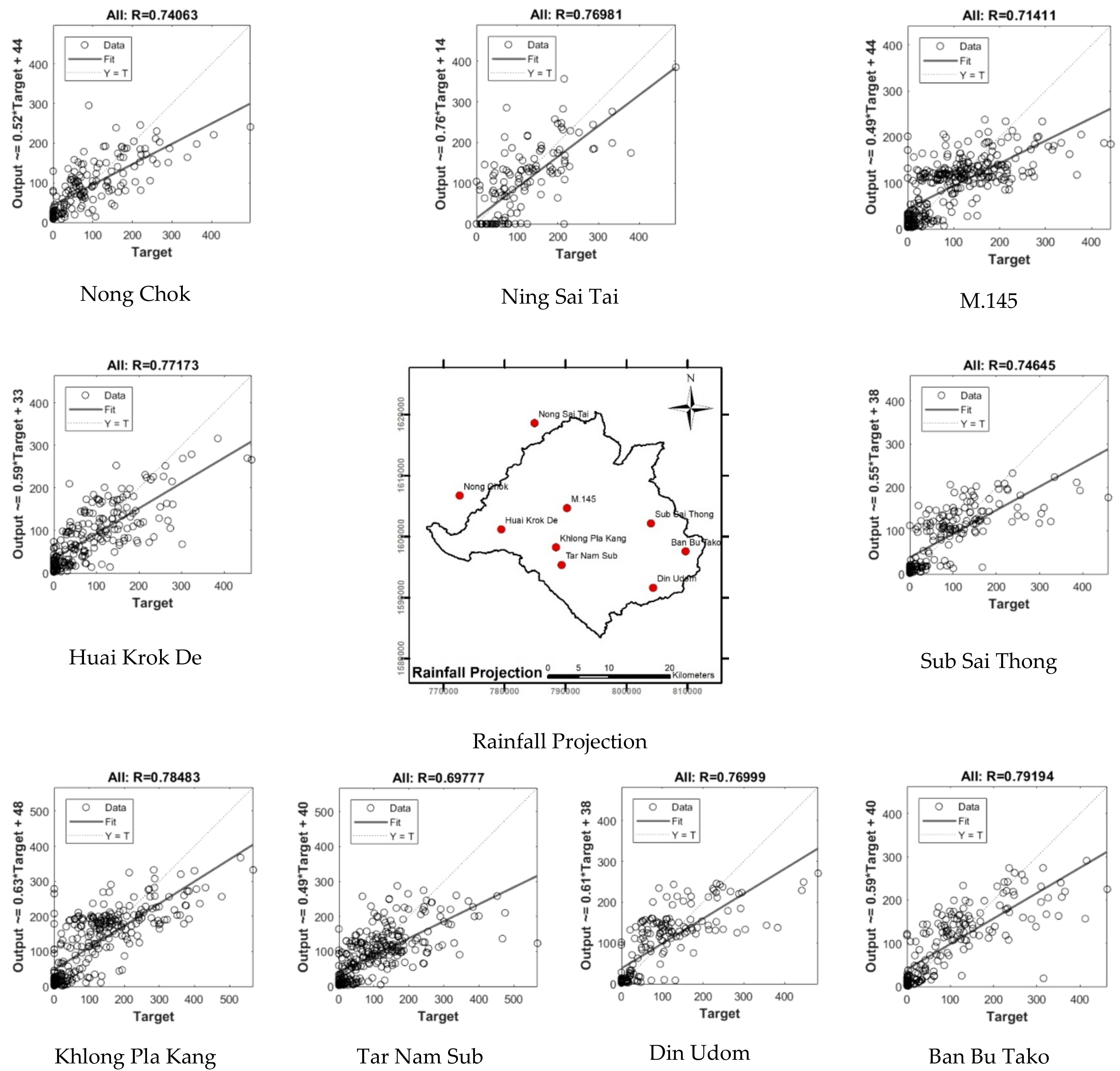
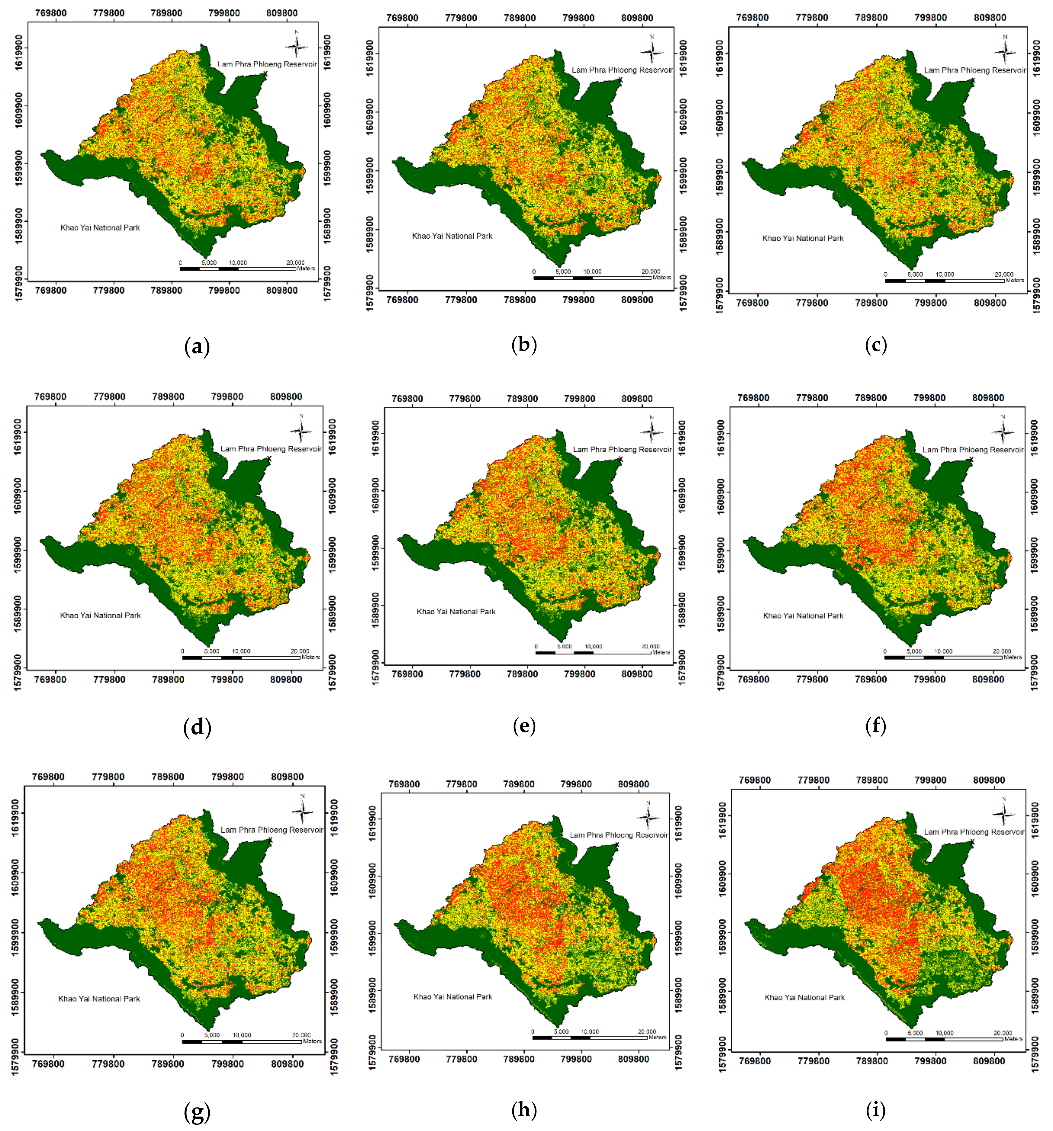
Future rainfall was simulated by combining the selected GCM and the ANN output. The model was calibrated and validated, before applying the soil erosion model. The average correlation coefficient, R², of each predicted rainfall data in every station was adjusted and validated to R² ≥0.70 by adjusting the number of layers and number of neurons in the back-propagation cascade network. Future soil loss was assessed for three future periods (near, mid, and far future) as shown in Figure 7 and Figure 8. Each climate scenario had a different rainfall pattern, and the varying R_m data was used in the USLE model.

Figure 7 shows the correlation of actual and projected rainfall under IPSL-CM5A-MR. The annual rainfall was predicted for all stations. The highest R² was 0.79 (Ban Bu Tako) and lowest R² was 0.70 (Tar Num Sub).

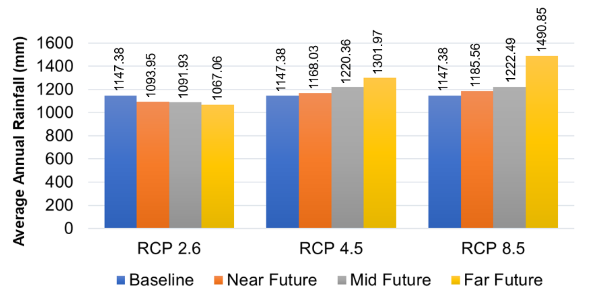
Figure 8 shows the projected average annual rainfall under IPSL-CM5A-MR. The rainfall in RCP 2.6 decreased in the near future and increased over time to the far future. Under RCP 4.5 and RCP 8.5, future rainfall increased over time from the near to the far future. This contributed to a change in the R_m factor in the USLE, leading to impacts on soil erosion and sediment yield.

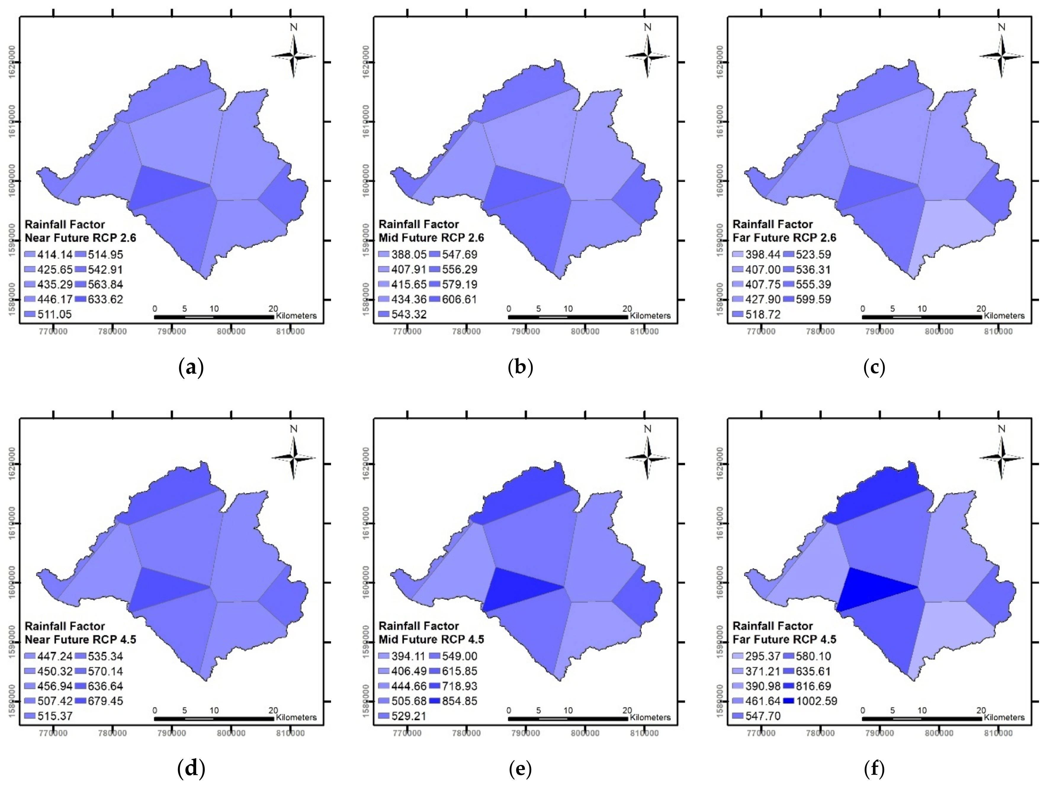
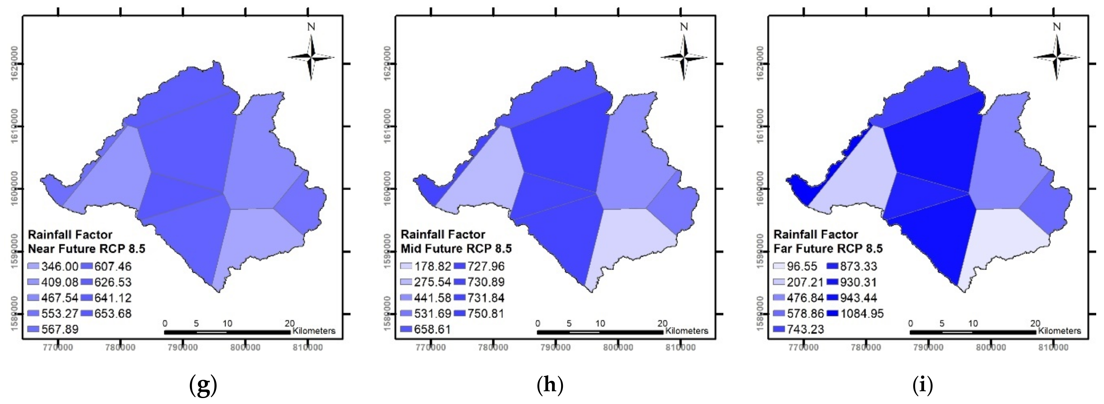
Figure 9 shows the R_m factor. Future rainfall was computed as R_m in the USLE, using Equation (2) and the Theisen polygon method. These figures show that R_m increased over time and the central part of the watershed had a very strong rainfall, so the soil should erode at the center of the dam. However, the R_m factor was not the only factor that controlled sediment in this watershed. The land cover and slope gradient were also significant. Future soil erosion and sediment yield under climate change should be confirmed by the USLE and SDR.

4. Result and Discussion

4.1. Estimate Long-Term Average Annual Soil Erosion

The distribution of the rainfall projections (RCP 2.6, 4.5 and 8.5) show a long-term change in average annual soil erosion. Accordingly, the long-term annual rainfall led to stronger soil erosion. Future periods were then labelled near, mid, and far future and compared with the past. Figure 10 and

Table 7. Results of estimated long-term average annual soil erosion.

Period	Soil Erosion Risk	Very Low	Low	Moderate	High	Very High
	t/km2/Year	(0–1250)	(1250–3125)	(3125–9375)	(9375–12,500)	(>12,500)
Baseline	Area (km2)	328.2	96.3	209.2	56.0	125.0
	% of Area	40.3	11.8	25.7	6.9	15.4
RCP 2.6	Area (km2)	333.3	101.6	213.5	53.5	112.7
Near Future	Change (%)	+0.63	+0.66	+0.53	−0.31	−1.51
RCP 2.6	Area (km2)	334.1	102.6	214.3	52.2	111.3
Mid Future	Change (%)	+0.73	+0.78	+0.63	−0.46	−1.68
RCP 2.6	Area (km2)	335.5	103.4	215.4	52.2	108.1
Far Future	Change (%)	+0.89	+0.87	+0.77	−0.46	−2.08
RCP 4.5	Area (km2)	326.6	94.1	206.9	55.4	131.6
Near Future	Change (%)	−0.19	−0.27	−0.29	−0.07	+0.81
RCP 4.5	Area (km2)	326.1	92.6	204.7	54.3	136.9
Mid Future	Change (%)	−0.26	−0.45	−0.55	−0.21	+1.45
RCP 4.5	Area (km2)	328.4	94.8	200.8	53.0	137.6
Far Future	Change (%)	+0.02	-0.18	−1.03	−0.36	+1.54
RCP 8.5	Area (km2)	324.2	93.1	203.3	54.6	139.5
Near Future	Change (%)	−0.49	−0.40	−0.73	−0.17	+1.78
RCP 8.5	Area (km2)	331.0	101.1	191.8	49.9	140.7
Mid Future	Change (%)	+0.34	+0.60	−2.13	−0.74	+1.92
RCP 8.5	Area (km2)	337.1	99.8	167.9	46.4	163.4
Far Future	Change (%)	+1.10	+0.43	−5.07	−1.17	+4.71

show long-term average annual rainfall for the entire watershed under the RCP 2.6, 4.5, and 8.5 scenarios for several periods. Under RCP 2.6, very low risk areas of soil erosion increased (≈2% of area), and very high risk areas decreased in the near, mid, and far future, the positions of these high risk area are a priority for water management and for plans to protect the LPP dam, since there is less rainfall in the center of the LPP and more in the evergreen forest area, and the average annual rainfall declined by about 4.8% (near), 4.8% (mid), and 7.2% (far).Under RCP 4.5, the average annual rainfall change, vs the baseline, was about +1.8% (near), +6.4% (mid), and +8.1% (far). These average rainfalls increased slightly, so rainfall caused erosion will similarly slightly. The strong rainfall was in the central part, which is consisted of lowland for agriculture, so the change in high and very high risk areas was 3%.

RCP 8.5 shows an extreme change in soil erosion risk in the far future, in the central part of the LPP watershed: the stronger rainfall at the middle point contributed to the increase in the very high risk of soil erosion. The rainfall in the middle increased by 25.4%, the very high risk areas increased by 4.7% and the moderate risk decreased by 5.1% compared to the baseline. Therefore, the priority of water management should be directed toward areas of moderate risk. Moreover, the strong rainfall increased to 22–25%, and these areas were scattered among the lowlands and hillslopes. RCP 8.5 in the far future showed significant changes compared to the baseline.

4.2. Predicted Sediment Yield in the LPP Reservoir

Different periods in the climate model showed varying sediment yields in the LPP reservoir, and these values were determined from the SDR multiplied by the total area of soil erosion, tabulated in

Table 8. Predicted sediment yield in the LPP reservoir.

Period	Predicted Sediment Yield
	Baseline	RCP 2.6		RCP 4.5		RCP 8.5
	(×103 t)	(×103 t)	Change (%)	(×103 t)	Change (%)	(×103 t)	Change (%)
Baseline	1148.1	-	-	-	-	-	-
Near Future	−	1069.9	−0.07	1060.9	−0.08	1040.9	−0.09
Mid Future	−	1188.9	+0.04	1250.6	+0.09	1196.9	+0.04
Far Future	−	1248.3	+0.09	1281.4	+0.12	1475.5	+0.29

. The eroded area varied with the topography and the climate model. The predicted sediment yield in the near, mid, and far future of RCP 2.6 was lower than the estimated baseline yield, due to the decrease in rainfall. The sediment yield for RCP 4.5 and RCP 8.5 was higher than the estimated baseline sediment.

5. Conclusions

Estimation of soil erosion in a watershed is necessary for water management and dam protection. We explored the interplay between the impact of climate change on soil erosion and sediment yield in the Lam Phra Phloeng (LPP) watershed using the Universal Soil Loss Equation (USLE) and the Sediment Delivery Ratio (SDR). The USLE is widely used for land cover management and organizations working in the environment, and the SDR is a ratio that defines the sediment delivery and sediment yield. The Global Climate model, by the Institute Pierre Simon Laplace-Climate Model version 5A (IPSL-CM5A-MR), was downscaled with Representative Concentration Pathways (RCPs) using an Artificial Neural Network (ANN). IPSL-CM5A-MR was selected here, because it correlated well, with low bias, with measured rainfall in the central part of Thailand. RCP 2.6 and RCP 8.5 were selected, as extremes in future rainfall, and RCP 4.5 was selected as representing the most likely rainfall in the central part of Thailand. Soil erosion was measured in the field to validate the USLE model. The error of average soil erosion in the LPP watershed between the USLE model and the field data was 4.0%. Thus, the USLE model is suitable for evaluating soil loss in this watershed.

At the baseline, soil erosion in the watershed was approximately 6000 t/km²/year, and the sediment yield in the reservoir was about 1148.1 × 10³ t. RCP 2.6 had lower rainfall, and RCP 4.5 and RCP 8.5 had higher rainfalls than the baseline. Interestingly, under RCP 2.6, the area with a very low risk of soil erosion increased, because the lower rainfall was in the field crop areas, which have a high opportunity for erosion, and the higher rainfall was in the evergreen forest areas, which present low soil erosion. The soil erodes and moves to the dam, so the dam has an increased service life. In contrast, under RCP 8.5, the moderate risk of soil erosion decreased, and the high and very high risk of erosion increased. These areas are scattered over the lowlands and hillslopes. The priority of water management should be to protect the moderate risk areas, so as to prevent them becoming high risk areas. The most likely scenario (RCP 4.5) showed a slight increase in soil erosion risk, because the strong rainfall was in field crop and horticulture areas. However, the high risk area was decreased by 0.2%, and the very high risk area was increased by 1.4%, so water management needs to prioritize high-risk areas.

Similarly, sediment yields in RCP 4.5 and 8.5 were increased 2.4% and 11.4%, whereas in RCP 2.6, it decreased to 10.7%, because the high rainfall was in the center of the watershed, which covered the river. The soil may then become eroded and transported to the LPP dam, so the service life of the dam will decrease. In addition, the impact of climate change on the SDR in the future is affected directly by annual rainfall and land cover. The rainfall directly affected soil loss - increased rain leads to higher soil erosion.

This study can be used to guide reservoir operation because changes in rainfall contribute to higher sediment delivery to, and dead storage in, the dams and a decreased service life. Green forest areas, as well as urban and farming areas should be protected from soil erosion.