The Role of Non-Hydrostatic Effects in Nonlinear Dispersive Wave Modeling

Abstract

Surface water waves is an important research topic in coastal and ocean engineering due to its influences on various human activities. In this study, our purpose is to gain a deeper insight on the effects of non-hydrostatic (NHS) pressure on surface wave motions and its role in numerical modeling, based upon the high-order NHS model and optional vertical accelerations. The relative contribution of non-hydrostatic effects (P_nhs/P_hs) and its sensitivity on phase celerity and amplitude of dispersive waves are quantified. The vertical structure of P_nhs/P_hs clearly indicates stronger NHS effects in deeper waters and its significance near the surface. The NHS effects mainly slow down wave celerity and maintain incident amplitude for linear dispersive waves. The NHS effects are also responsible for increased amplitude and phase speed under strong non-linearity. The inter-relation between (un)realistic physical responses and model errors is discussed. Further, four experimental conditions for waves with complicated interactions are examined. Overall, the NHS effects play a critical role in side-band generation of bi-chromatic waves, and increased celerity and amplitude during nonlinear shoaling, as well as velocity moderation under co-existence of depth-varying currents. Possibly owing to weaker wave–wave interactions, however, wave directionality does not strongly interfere with FNHS/QNHS (Fully/Quasi Non-HydroStatic) effects on a fast-modulated nonlinear evolution of spatial focusing or diffraction waves.

1. Introduction

Surface water waves with significant influences upon human activities is an important research topic in the field of coastal and ocean engineering [1,2,3]. In the past several decades, analytical and experimental efforts [4,5,6] have been made to reveal basic characteristics of surface wave motions. Driven by the horizontal gradient of non-hydrostatic pressure (associated with vertical acceleration of fluid), dispersion is the most essential feature in wave propagation (i.e., longer waves traveling faster than shorter waves in a wave group) [4]. Besides, nonlinear transformation can arise owing to (mutual or self) interactions among larger wave components, such as the formation of side-band or higher harmonics in deep or shallow waters [1,4,6,7,8,9,10]. A Doppler shift in dispersion can also be found if there are currents co-existing with waves [11,12]. In the meantime, along with theoretical works, a great amount of effort has also been devoted to surface wave modeling [13,14,15]. Accordingly, complicated wave motions in more realistic conditions (e.g., combination of shoaling, refraction, and diffraction over irregular bottom) can be resolved. However, proper representations of dispersion and nonlinearity required for accurate and efficient wave modeling are challenging [14]. With a solid background from the literature, this study aims at gaining a further and deeper insight into the role of non-hydrostatic effects in complicated wave transformation. In particular, a better understanding of the detailed contribution of non-hydrostatic pressure effects would assist continuous development and applications of nonlinear dispersive wave modeling.

To date, according to the vertical dimension treatment in governing equations, wave modeling frameworks can be classified into two major groups: (i) depth-integrated models, including Boussineq equation (e.g., [16,17,18,19,20,21]), mild-slop equation (e.g., [22,23,24]), and their variants, as well as (ii) the multi-layer models based on Laplace’s equation derived from the potential flow theory with irrotational assumption (e.g., [25,26,27,28,29,30]), and the complete Navier-Stokes equations (e.g., [31,32,33,34,35,36]). In the former group, subject to limited computer capacity in the 1970s, the classical Boussinesq-type equation [16] and mild-slope equation [22] utilize a polynomial and depth integration factor to describe the velocity profiles for weakly nonlinear dispersive waves and linear waves over an entire range of depth, respectively. The constrains have been relaxed by several approaches, such as the optimal expansion levels, higher-degree polynomials, higher-order derivatives, and multiple layers [17,18,19,20,21,23,24]. In contrast to depth integration, with the vertical structure of pressure and velocity (potential) fields, accurate description of nonlinear dispersive waves can be achieved naturally, since the non-hydrostatic pressure has been directly included. Without any approximations or assumptions, non-hydrostatic modeling is the most general approach, especially for flows involving shear, vortex, and turbulence [37,38,39]. A theoretical framework for the interpretation of wave dispersion/nonlinearity in non-hydrostatic models can refer to Bai and Cheung [40]. However, a demanding computation was typically required in non-hydrostatic modeling.

In the last decade, non-hydrostatic modeling has been intensively studied to obtain improved accuracy and better efficiency for a broader range of surface wave motions (e.g., [15,39,41,42,43,44,45,46,47,48,49,50,51,52,53]). Unlike conventional models that simply addressed non-hydrostatic pressure for the lower computational cells [31,32,33,34,35,36], efficient models implemented the top-layer non-hydrostatic pressure treatments in various ways, such as the Kellor-box scheme [41,42], the integral method [15,43,44,45], the interpolation method [46,47], or several others (see the references in Young and Wu [50]). As a consequence, these models using only 2–5 layers (one order of magnitude less) can precisely simulate steep (aK = 0.30, where a is the amplitude and K is the wave number) wave propagation within dimensionless relative water depth Kh = 5 (where h represents still water depth) at 1% tolerance phase error [42,45,47]. Young and Wu [51] further modified the top-layer pressure treatment based upon a cubic function with a fourth-order truncation error, providing a highly accurate and efficient non-hydrostatic (NHS) model for various wave problems (dispersive degree up to Kh = 15). Success of these models facilitates further detailed analysis on the non-hydrostatic effects.

In earlier works, the non-hydrostatic effects on surface wave motions were demonstrated simply by using a qualitative comparison (i.e., a noticeable discrepancy) between the prediction and analytical solutions (e.g., [34,35]). Chen [54] further quantified hydrostatic and non-hydrostatic components for linear seiche oscillations. The scale analysis indicated that the non-hydrostatic pressure gradient was not necessarily small, although the non-hydrostatic pressure was about 2–3 orders of magnitude smaller than the hydrostatic component. For wave transformation with various dispersion/nonlinearity and complicated interactions (among waves, bottoms, and currents, as well as directionality); however, the role of non-hydrostatic effects has not yet been characterized, as far as the authors are aware.

The objective of this paper is to clearly identify the effects of non-hydrostatic pressure on surface wave motions and its important role in numerical modeling. Based upon the high-order NHS model [49,51], the non-hydrostatic contributions are quantified by optional vertical accelerations, that is, hydrostatic (HS, no acceleration), quasi non-hydrostatic (quasi non-hydrostatic defined in this paper is different from “quasi hydrostatic”, which represents the surface calculation step of the pressure-split algorithm in a fully non-hydrostatic model [55]), (QNHS, local acceleration only), and fully non-hydrostatic (FNHS, local and convective acceleration). Specifically, the normalized vertical profile of non-hydrostatic pressure (P_nhs/P_hs) and its effects on wave celerity and amplitude are examined against the linear and non-linear analytical solutions. Further, the non-hydrostatic effects on complicated wave problems are elucidated using the high-order NHS model and available experiments, that is, non-linear bi-chromatic waves in deep water, non-linear wave shoaling, non-linear waves interacting with a depth-varying current, and 3D focusing/diffracting waves.

2. Model Description

The non-hydrostatic model [49,51] solves the unsteady, incompressible, Navier–Stokes equations to simulate free surface wave motions based on the staggered finite difference Crank–Nicholson scheme in the transformed σ domain (see Figure 1). The implicit numerical algorithm relaxes the stability restriction of computational time-steps in comparison to the explicit ones. Besides, the algorithm treats a 3D problem as a series of 2D vertical planes to yield block hepta-diagonal system matrixes that can be solved directly without iterations. The boundary-fitted co-ordinate $\sigma =(z^{\ast }-\eta )/(h+\eta )$ ensures an accurate representation of the free surface elevation (i.e., $z^{*}=\eta$ or $\sigma =0$) and the irregular bottom topography (i.e., $z^{*}=-h$ or $\sigma =-1$). Most importantly, the higher-order top-layer pressure treatment based upon a cubic polynomial interpolation can accurately resolve phase velocity. The developed NHS model has been carefully validated against either analytical solutions or experimental data for various wave problems from shallow to deep water depth [49,51], clearly demonstrating the model’s efficiency (requirement of only 2–5 vertical layers) and accuracy (dispersive degree up to Kh = 3–15).

In the following, the model description including the governing equations and numerical algorithm is briefly presented here. Details can refer to Young et al. [49] or Young and Wu [51]. The transformed 3D governing equations can be written as

$$\left(\frac{\partial u}{\partial x}+\frac{\partial u}{\partial \sigma }\frac{\partial \sigma }{\partial x^{*}}\right)+\left(\frac{\partial v}{\partial y}+\frac{\partial v}{\partial \sigma }\frac{\partial \sigma }{\partial y^{*}}\right)+\left(\frac{\partial w}{\partial \sigma }\frac{\partial \sigma }{\partial z^{*}}\right)=0,$$

(1)

$$\frac{\partial u}{\partial t}+u\frac{\partial u}{\partial x}+v\frac{\partial u}{\partial y}+w_{\sigma }\frac{\partial u}{\partial \sigma }=-\left(\frac{\partial P}{\partial x}+\frac{\partial P}{\partial \sigma }\frac{\partial \sigma }{\partial x^{*}}\right)+v{\nabla }_{\sigma }^{2}u,$$

(2)

$$\frac{\partial v}{\partial t}+u\frac{\partial v}{\partial x}+v\frac{\partial v}{\partial y}+w_{\sigma }\frac{\partial v}{\partial \sigma }=-\left(\frac{\partial P}{\partial y}+\frac{\partial P}{\partial \sigma }\frac{\partial \sigma }{\partial y^{*}}\right)+v{\nabla }_{\sigma }^{2}v,$$

(3)

$$\frac{\partial w}{\partial t}{\delta }_l+\left(u\frac{\partial w}{\partial x}+v\frac{\partial w}{\partial y}+w_{\sigma }\frac{\partial w}{\partial \sigma }\right){\delta }_c=-\frac{\partial P}{\partial \sigma }\frac{\partial \sigma }{\partial z^{*}}+v{\nabla }_{\sigma }^{2}w-g,$$

(4)

with

$$w_{\sigma }=\frac{\partial \sigma }{\partial t^{*}}+u\frac{\partial \sigma }{\partial x^{*}}+v\frac{\partial \sigma }{\partial y^{*}}+w\frac{\partial \sigma }{\partial z^{*}},$$

$${\nabla }_{\sigma }^2=\frac{{\partial }^2}{\partial x^2}+2\left(\frac{\partial \sigma }{\partial x^{*}}\right)\frac{{\partial }^2}{\partial x\partial \sigma }+\frac{{\partial }^2}{\partial y^2}+2\left(\frac{\partial \sigma }{\partial y^{*}}\right)\frac{{\partial }^2}{\partial y\partial \sigma }+\left[{\left(\frac{\partial \sigma }{\partial x^{*}}\right)}^2+{\left(\frac{\partial \sigma }{\partial y^{*}}\right)}^2+{\left(\frac{\partial \sigma }{\partial z^{*}}\right)}^2\right]\frac{{\partial }^2}{\partial {\sigma }^2},$$

where the superscript asterisk indicates the physical domain; u, v, and w are the velocity components; P is the normalized pressure divided by a constant reference density; g is the gravitational acceleration; ν is the kinematic viscosity; and δ_l and δ_c are the optional flags for the vertical accelerations to determine the HS, QNHS, and FNHS experimental conditions.

Several boundary conditions are required to solve the Equations (1)–(4). At the bottom boundary, a kinematic condition for a fixed bed is applied. For the free surface, a conservative form of the free-surface equation that results from the integration of the continuity equation over the water depth with associated kinematic conditions can be expressed as

$$\frac{\partial \eta }{\partial t}+\frac{\partial }{\partial x}\left(H{\displaystyle {\int }_{-1}^{0}ud\sigma }\right)+\frac{\partial }{\partial y}\left(H{\displaystyle {\int }_{-1}^{0}vd\sigma }\right)=0,$$

(5)

where $H=h+\eta$ is the total water depth. In addition, the continuity of normal stress is enforced, that is, $P{|}_{\sigma =0}=P_a$, where $P_a$ is the atmospheric pressure and taken as zero here. Notice that the staggered pressure is arranged at the center of the top layer rather than the free surface. Using the integral method [15,43,44,45,49,51], the top-layer pressure boundary condition can be derived as

$$P=\frac{gH\Delta {\sigma }_K}{2}+{\delta }_l\frac{\partial }{\partial t}{\displaystyle {\int }_{{\sigma }_K}^{0}Hwd\sigma }+{\delta }_c\left(\frac{\partial }{\partial x}{\displaystyle {\int }_{{\sigma }_K}^{0}Huwd\sigma }+\frac{\partial }{\partial y}{\displaystyle {\int }_{{\sigma }_K}^{0}Hvwd\sigma }-H{w}_{\sigma }w{|}_{\sigma ={\sigma }_{\mathrm{K}}}\right),$$

(6)

consisting of the hydrostatic component caused by the free-surface elevation (i.e., the first term on the right-hand side) and the non-hydrostatic one attributed to the vertical acceleration (i.e., the rest terms). At the inflow boundary, the horizontal velocity component with a ramp function is specified to generate waves without the undesired noises due to an impulse motion [41,45]. For the outflow boundary, a combination of the sponge layer technique and the Sommerfeld radiation boundary condition is used to minimize wave reflection [44].

The model domain can be discretized by a set of computational cells with non-uniform (or uniform) grid-spacing along each direction (Figure 1). The velocity and pressure variables are defined under a staggered grid system. The overall numerical algorithm consists of three major steps. First, the discretization step applies the Crank–Nicholson scheme to the continuity equation, momentum equations, and free-surface equation, expressing the vertical velocity, and free-surface elevation as functions of horizontal velocities and providing the relation of the lower-layer pressure to its upper one and adjacent velocities. Second, pressure treatment step uses Equation (6) to specify the top-layer pressure. Particularly, a cubic function with fourth-order truncation error is employed to address the vertical profile of dispersive waves for better accuracy. With the top-layer pressure and the relation between each layer, the pressure over the entire depth can be represented as a function of horizontal velocities. Third, the solving step solves the horizontal velocities in each vertical plane from the block hepta-diagonal system matrix, which is obtained by eliminating the vertical velocity and pressure in the discretized horizontal momentum equations and is then solved using an efficient direct matrix solver. The rest variables can be simultaneously obtained by simple back-substitution.

3. Non-Hydrostatic Effects on Linear/Nonlinear Waves

In the following, the relative contribution (P_nhs/P_hs) and sensitivity of non-hydrostatic effects on the phase celerity and amplitude in linear/nonlinear dispersive waves are examined.

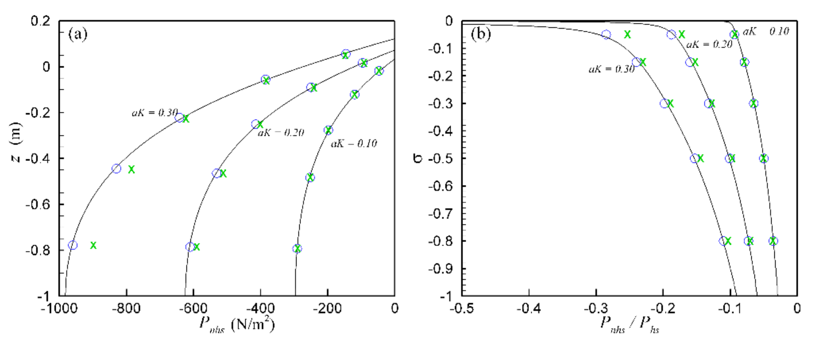
3.1. Linear Wave Dispersion

Linear (frequency) dispersion means that water waves with different wavelengths λ (or wave periods T) propagate at different phase speeds c in a given depth h [1]. Incident wave conditions with infinitesimal amplitude (a/h = 0.001) and four dimensionless water depth Kh (ranging from shallow to extremely deep-water depth, i.e., Kh = π/25, π/5, π, and 5 π) are considered here. We conduct numerical experiments in a vertical 2D tank (Figure 2) with a length L = 10λ and an undisturbed water depth h = 1 m. A sponge layer with a length $L_{SP}=2\lambda$ is employed to avoid reflection. The simulation is carried out with 40 grids per wave length along the x direction and “stretched” five vertical layers [31]. The time-step Δt is determined by setting the Courant number Cr = cΔt/Δx = 0.5. The viscosity is set to zero.

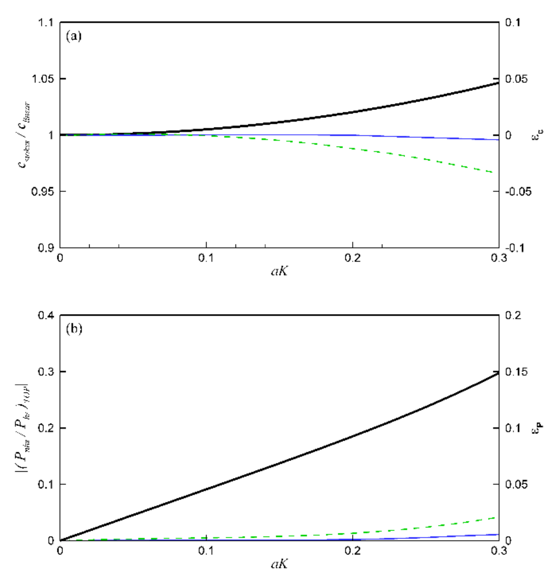
3.1.1. Contribution and Sensitivity Analysis

The vertical profile and relative contribution of non-hydrostatic pressure are analyzed here, instead of a qualitative comparison of pressure contours [34,35,44] or pressure time-series [56] in most previous works. As shown in Figure 3a, the HS condition reveals no non-hydrostatic pressure and the FNHS/QNHS distribution under the crest perfectly agree with the analytical solutions for all four different conditions of Kh. In comparison to the horizontal velocity that has a positive profile with a maximum at z^* = η (not shown here), the magnitude of the negative non-hydrostatic pressure remains zero at the free surface and then increases along the depth. Sharper variations appear in the deeper water conditions (e.g., Kh = 5π). Figure 3b compares the non-hydrostatic pressure (P_nhs) with the hydrostatic component (P_hs). The orders of a relative ratio P_nhs/P_hs are O(10⁻⁵–10⁻²) from Kh = π/25 to Kh = 5π, showing that the non-hydrostatic pressure is influential, especially in the dispersive deep-water waves. In addition, the location of the maximum contribution of P_nhs occurs near the surface.

Subsequently, the role of non-hydrostatic pressure in wave propagation speed is revealed in Figure 4. As the dispersive degree increases, the stronger non-hydrostatic effects lead to a decreased phase speed (see black lines). In terms of sensitivity, we consider the variation of phase speed in response to the change of non-hydrostatic pressure. Apart from the hydrostatic condition, the phase speed of intermediate-water waves (π/10 < Kh < π) reduces from (gh)^1/2 to 0.56 (gh)^1/2, while the relative contribution P_nhs/P_hs increases from O(10⁻⁵) to O(0.003). In the cases of deep-water waves (up to Kh = 20), the wave celerity keeps decreasing down to 0.22 (gh)^1/2 as the P_nhs/P_hs ratio grows to O(0.012).

In addition to the physical response, model errors (calculated from the simulated free surface elevation) may interfere in the aforementioned relationship. Two relative errors for the phase speed and top-layer non-hydrostatic pressure are also shown in Figure 4, that is, ${\epsilon }_c=(c_{\mathrm{model}}-c_{\mathrm{exact}})/c_{\mathrm{exact}}$ and ${\epsilon }_P=\left|{\left(P_{nhs}\right)}_{TOP}^{\mathrm{model}}-{\left(P_{nhs}\right)}_{TOP}^{\mathrm{exact}}\right|/\rho g\eta$ (see blue lines for the identical FNHS/QNHS results). It can be found that the five-layer NHS model shows great accuracy for a wide range of dispersive degree (up to Kh = 5π). Compared to earlier works (e.g., [31,45]), the high-order top-layer pressure treatment is proved to be critical for efficient and accurate modeling, although the ratio (P_nhs/P_hs) is small (e.g., O(10⁻⁵–10⁻²)). As the dimensionless water depth increases up to 20 (or the top-layer P_nhs/P_hs > 0.01), the 3% error in the non-hydrostatic pressure leads to a 6% under-estimation of phase speed. Such an accuracy issue in the extremely deep-water conditions can be tackled by using more vertical layers or higher-order numerical treatment in NHS or Boussinesq-type models (e.g., see [21]).

3.1.2. Free-Surface Spatial Profile

For a better understanding of the non-hydrostatic effects on wave celerity and amplitude, the predicted free-surface spatial profiles are demonstrated in Figure 5. For different water depths (i.e., Kh = π/25 − 5π), both FNHS and QNHS simulations are in excellent agreement with the analytical solutions. Almost identical results indicate that the local vertical acceleration dominates the behavior of linear waves. The role of non-hydrostatic pressure is further revealed through the comparison of the HS condition. While appropriate for shallow water (Kh = π/25), neglecting the NHS effects leads to unrealistic long-wave patterns once the dimensionless water depth increases (Kh > π/5), that is, in regard to the over-predicted wavelength and underestimated amplitude. Such discrepancies can be physically explained using the concepts of phase velocity and energy flux [4]. For a deep-water condition (Kh = π), the incident wave with a theoretical phase speed 0.56 (gh)^1/2 is forced to propagate at the speed of (gh)^1/2 toward the downstream of the HS numerical tank. As a consequence, the faster celerity yields the longer wavelength (i.e., λ_HS = 1.77 λ_Inc). Further, the energy flux should be conserved between the incident boundary and any given location in the tank. Substituting the theoretical and HS group velocity C_g into ${(\rho g{H}^2{C}_g)}_{Inc}={(\rho g{H}^2{C}_g)}_{HS}$, one can easily obtain a smaller wave height H_HS = 0.54 H_Inc (or a_HS = 0.27 H_Inc). Overall, the results indicate that the NHS effects attributed to the vertical acceleration would slow down celerity and remain incident amplitude for dispersive waves.

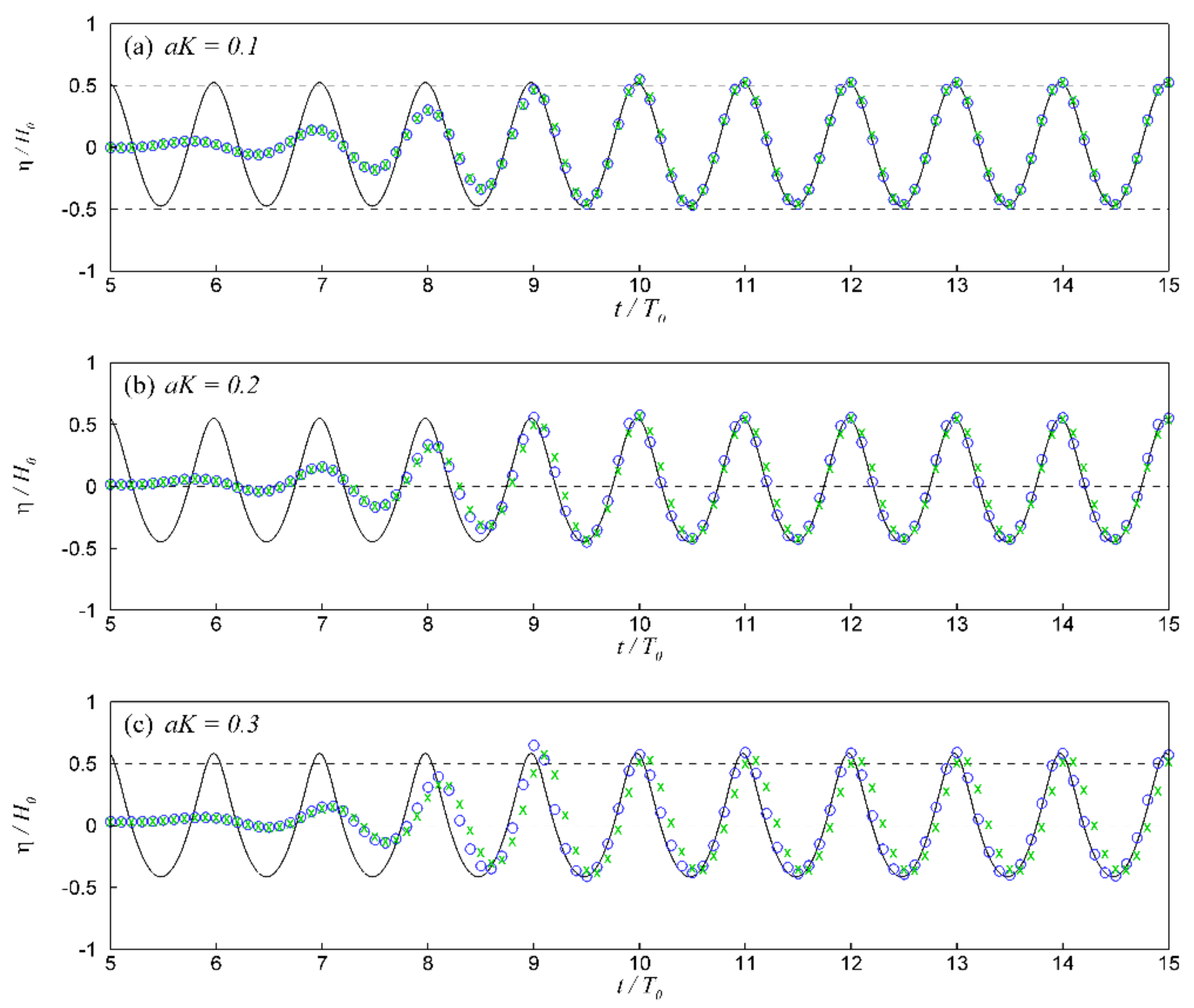
3.2. Wave Non-Linearity

We further consider the propagation of non-linear deep-water (Kh = π) wave that can be characterized by different wave steepness (i.e., ε = aK = 0.10, 0.20, and 0.30). The HS condition is inapplicable and not discussed here. To examine the non-hydrostatic effects, the FNHS and QNHS simulations will be compared against the fifth-order Stokes theory [5], that is,

$$\begin{array}{cc}\hfill K\eta =& a_1\cos [K(x-ct)]+a_2\cos [2K(x-ct)]+a_3\cos [3K(x-ct)]\hfill \\ \hfill +& a_4\cos [4K(x-ct)]+a_5\cos [5K(x-ct)]\hfill \end{array}$$

(7)

$$c=\sqrt{g/K}[1+\frac{1}{2}{\epsilon }^2+\frac{1}{8}{\epsilon }^4]$$

(8)

where the coefficients are $a_1=\epsilon -\frac{3}{8}{\epsilon }^3-\frac{211}{192}{\epsilon }^5$; $a_2=\frac{1}{2}{\epsilon }^2+\frac{1}{3}{\epsilon }^4$; $a_3=\frac{3}{8}{\epsilon }^3+\frac{99}{128}{\epsilon }^5$; $a_4=\frac{1}{3}{\epsilon }^4$; and $a_5=\frac{125}{384}{\epsilon }^5$.

3.2.1. Contribution and Sensitivity Analysis

Similarly, the vertical profile and relative ratio of non-hydrostatic pressure are compared in Figure 6. In general, the overall features are quite close to those in the linear cases, except for the larger magnitude O(10²) and slightly different contribution pattern near the surface. While the local vertical acceleration is dominant, the convective one plays a non-negligible role in the non-hydrostatic pressure for the cases of strong non-linearity (see the shifted profile and under-estimated top-layer significance as aK increases to 0.20 or 0.30).

Subsequently, Figure 7 compares the wave celerity and top-layer non-hydrostatic pressure versus wave steepness (rather than dimensionless water depth in those linear cases). As the degree of nonlinearity extends, the stronger non-hydrostatic effects yield an increased phase speed. For the highly non-linear case (aK = 0.30), the wave celerity and the contribution ratio P_nhs/P_hs increase to about 1.05 c_linear and 0.30, respectively. The FNHS pressure representation fully considers the vertical acceleration, and thus yields precise phase speed for Stokes waves (i.e., ε_c < 0.5%). Dropping the physics of convective effects, the QNHS mode creates 2% error in the non-hydrostatic pressure, leading to 3% under-estimation in non-linear wave celerity (computed from the simulated free surface elevation).

3.2.2. Free-Surface Time Series

Figure 8 compares the modeled time series of free-surface displacement at x = 3λ for a better visualization. The FNHS simulation can accurately resolve the nonlinear wave celerity and vertically asymmetric wave profile with η_crest/H_Inc = 0.58 (or η_trough/H_Inc = −0.42) for wave steepness up to aK = 0.30, consistent with Figure 6 of Yuan and Wu [45]. The full influence of non-hydrostatic pressure can be observed from the difference between FNHS and QNHS results. The QNHS mode gives smaller non-hydrostatic effects (see Figure 6), further affecting wave amplitude and phase speed, especially under stronger non-linearity. Without convective vertical acceleration, the free-surface elevation presents decreased wave steepness in the simulation results, that is, ε = aK ≈ 0.20 (or η_crest/H_Inc ≈ 0.55). The resulting phase speed in the QNHS prediction can be explained using the Stokes theory [5]. According to Equation (8), the nonlinear incident waves with smaller ak would propagate at only 97% of phase speed c (see 3% error in Figure 7 or the lagged time series in Figure 8c) when traveling to the downstream of the QNHS numerical tank. In other words, the fully NHS effects considering both local and convective vertical acceleration would increase the wave steepness (or amplitude), as well as propagation speed for nonlinear waves.

4. Non-Hydrostatic Effects for Waves with Complicated Interactions

In this section, the non-hydrostatic effects on complicated wave problems are further elucidated using the high-order NHS model and available experiments, that is, non-linear bi-chromatic waves in deep water, non-linear wave shoaling, non-linear wave interacting with a depth-varying current, and 3D focusing/diffracting waves.

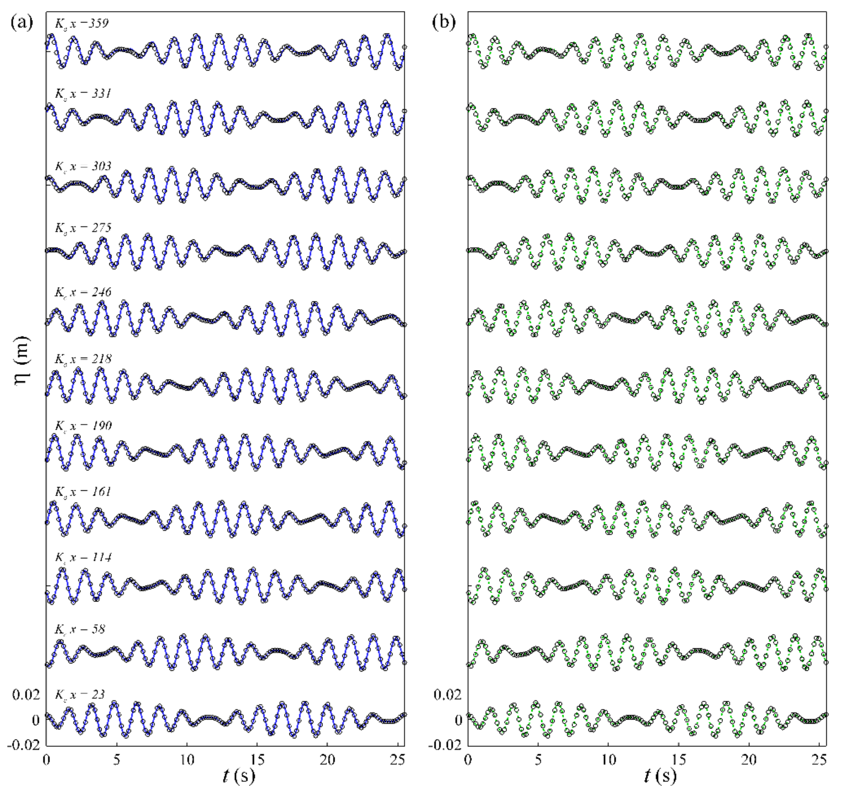
4.1. Bi-Chromatic Waves

We choose the laboratory experiment of bi-chromatic waves [9] to demonstrate the FNHS/QNHS pressure effects on the evolution of a nonlinear deep-water wave group with strong wave–wave interactions. The non-breaking case B11 [57] is considered, while its wave amplitude and phase speed were not easily resolved using the multi-layer Boussinesq model [21] and fourth-order non-linear Schrödinger equation [58].

According to the experimental setting of Hwung and Chiang [9], the numerical wave tank is 300 m long with an undisturbed water depth of 3.5 m. A sponge layer is used to replace the wave-absorbing beach. The incident waves consist of the low- and high-frequency components with periods of T_l = 1.7 s and T_h = 1.5 s (K_lh = 4.87 and K_hh = 6.26). The imposed wave heights are the same, that is, H = 0.1 m (aK_l = 0.070 and aK_h = 0.089). The computation domain is discretized by 1500 uniform horizontal cells (Δx = 0.2 m) and five stretched vertical layers. The time step is determined by setting Cr = cΔt/Δx = 0.1, where c is defined as (gh)^1/2. The total simulation time is 400 s.

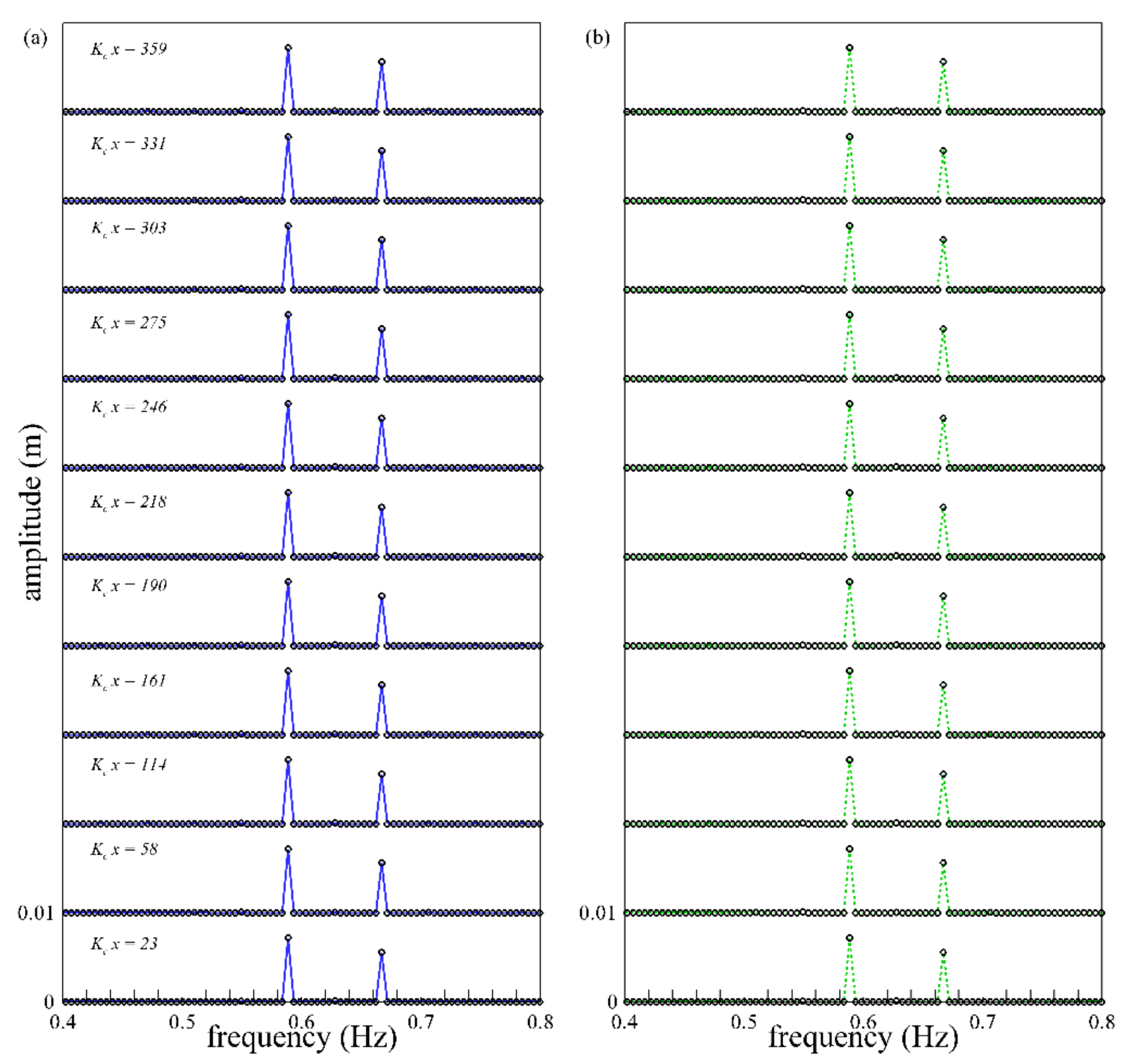
4.1.1. Linear Bi-Chromatic Waves

We firstly carry out a linear benchmark case with exactly the same periods but smaller amplitude (a_lK_l = a_hK_h = 0.01). Figure 9 compares the simulated free surface time series with the second-order analytical solution [59] at 11 gauge stations from the dimensionless distance K_c x = 23 to K_c x = 359, where K_c is the wave number obtained using the mean wave period T_m = 1.6 s. As it can be seen, the two components of the bi-chromatic waves travel to the downstream in symmetric groups with a period of 25.5 s. Figure 10 shows the predicted amplitude spectrum with signals only at the base frequencies. Overall, both FNHS and QNHS simulations (with similar dispersion capability) excellently describe the linear wave group since almost no wave–wave interactions occur and dispersive effects are dominant in such a small amplitude case.

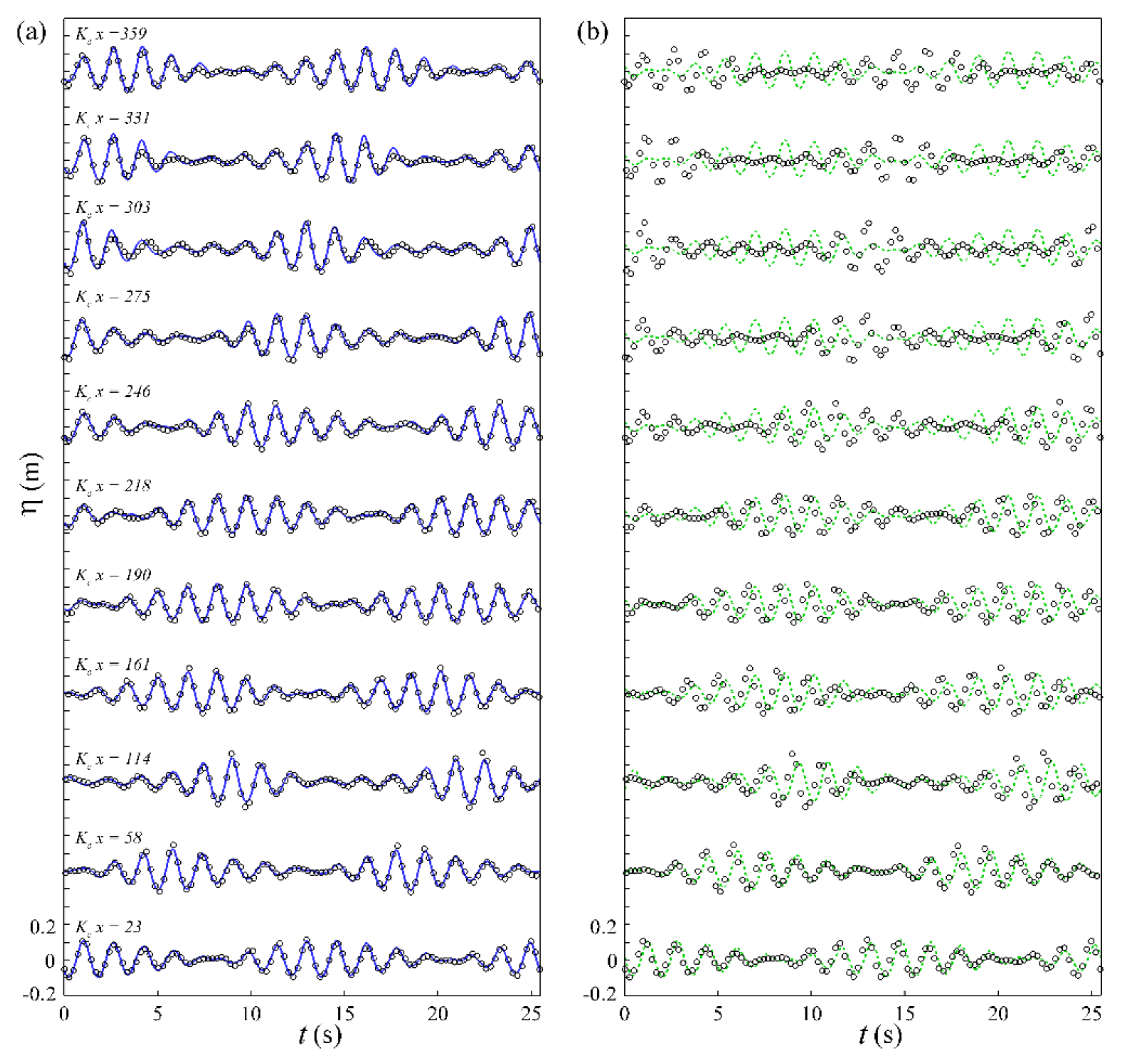
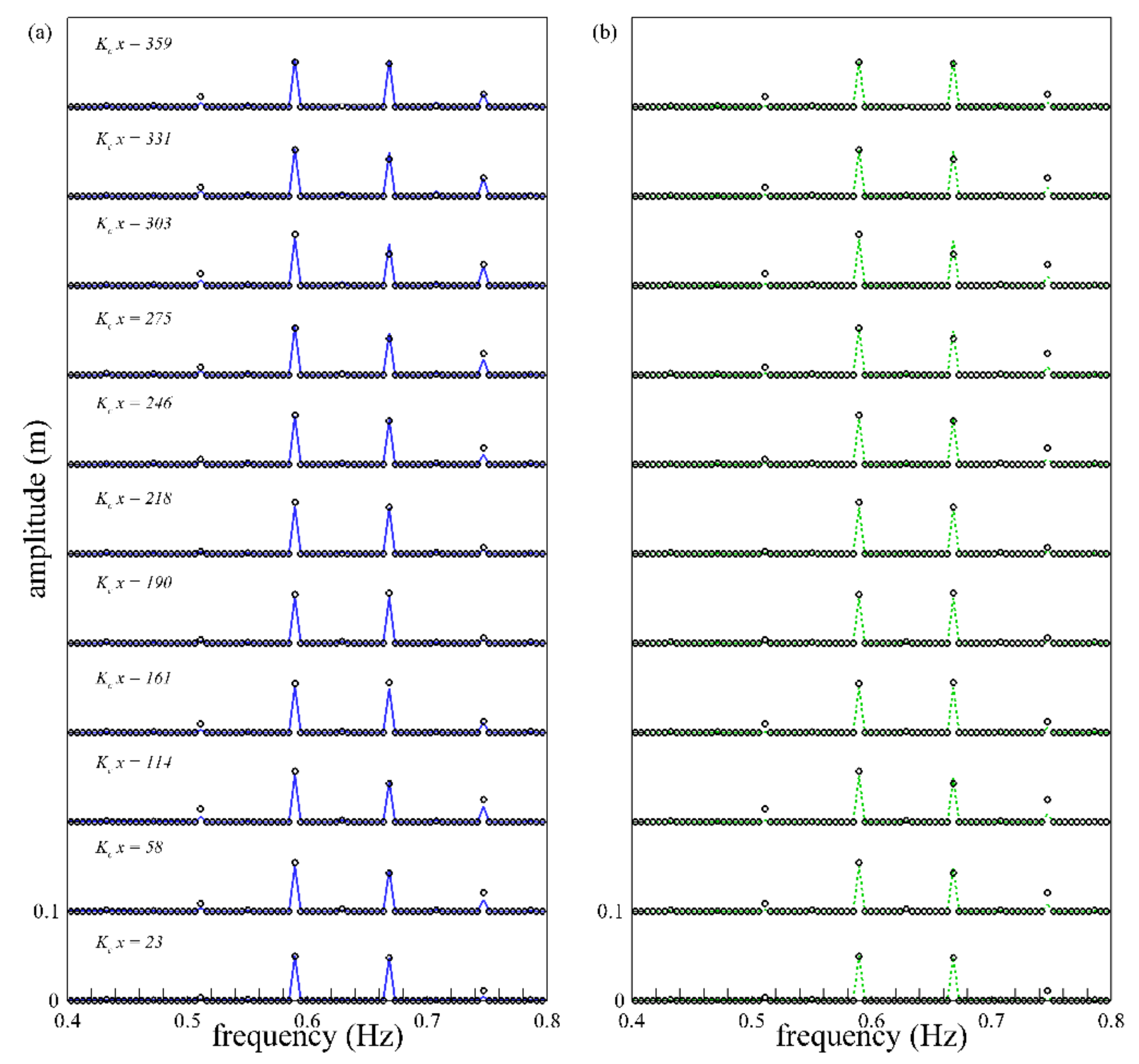
4.1.2. Non-Linear Bi-Chromatic Waves

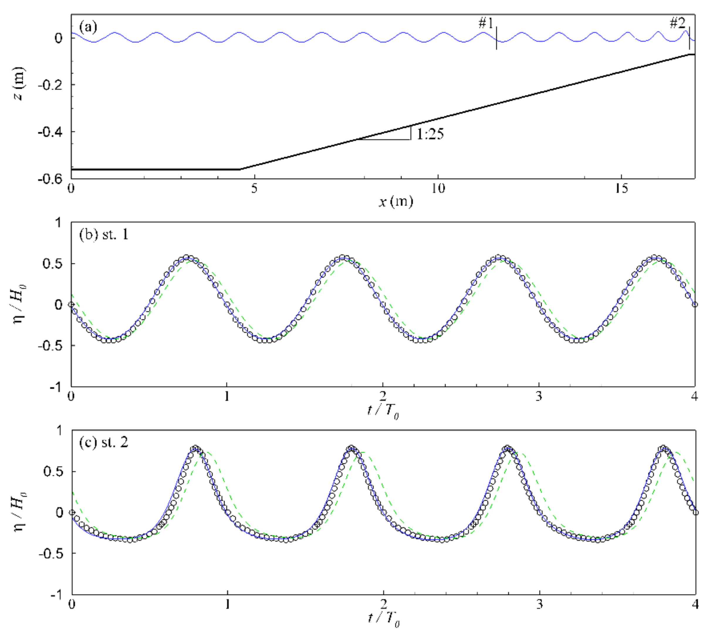
For the non-linear experimental condition, Figure 11 compares the predicted wave profiles with the observation data. The second-order solution is not adopted due to its difficulty in representation of energy redistribution [60]. The FNHS results reasonably capture the evolution of non-linear bi-chromatic waves. It can be clearly seen that the initial wave trains resemble a linear superposition of two imposed wave components (K_c x = 23). As the wave trains travel to the downstream, a strong asymmetric envelope with steep fronts and gently sloping rears (K_c x = 58) forms, consistent with several other experimental results [58,61,62]. Afterward, the wave energy is focused into the center of the wave groups (K_c x = 114), followed by the recurrence of the initial stage (K_c x = 161). The processes of modulation and de-modulation cyclically repeat until the end of the tank. Figure 12 further shows the predicted spectrum with two side-band components (2ω₁ − ω₂, 2ω₂ − ω₁) evolved from the non-linear interactions between the base frequencies. The QNHS mode without the convective vertical acceleration would under-estimate both wave amplitude and phase speed of the non-linear incident wave group, as discussed in Section 3.2. Moreover, the side-band frequencies are hardly captured (see Figure 12b). Therefore, the evolution of non-linear bi-chromatic waves in the QNHS numerical tank is unrealistic (see noticeable phase lag and 20% smaller amplitude at the center of wave groups at the distance of K_c x = 114 in Figure 11b). Based upon a multi-layer Boussinesq model and fourth-order non-linear Schrödinger equation, such a discrepancy due to under-estimated wave amplitude and/or phase speed has also been reported [21]. Overall, the role of FNHS pressure in wave–wave interactions is apparently revealed.

4.2. Wave Shoaling

Subsequently, we consider the experiments conducted by Nwogu [18] to observe FNHS/QNHS effects on wave transformation over a sloping bottom. The numerical tank is 20 m long with a 1:25 beach placed at x = 4.6 m, and the still water depth is 0.56 m (see Figure 13d). A sponge layer (at the last 2 m of the tank) is used to represent the experimental wave absorber. The incident conditions are T = 0.85 s (Kh = 3.13) and H₀ = 0.04 m (aK = 0.11). The computational domain is discretized by a set of horizontally uniform cells (i.e., Δx = 0.05 m) and five vertically stretched layers. The time-step is determined by setting Cr = 0.5.

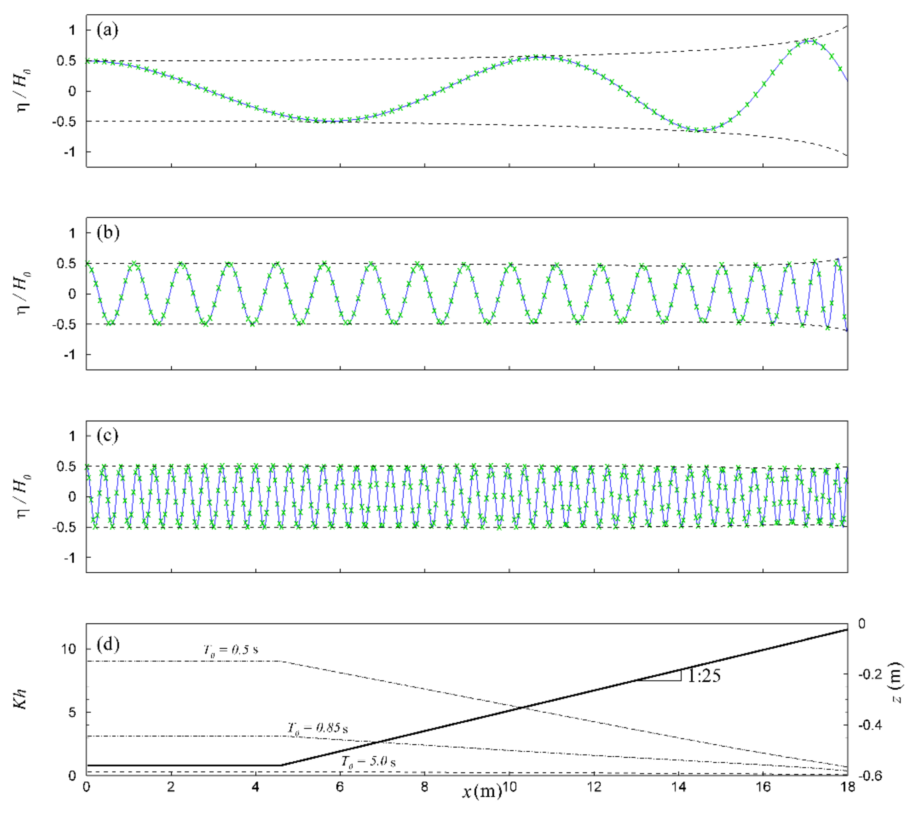
4.2.1. Linear Wave Shoaling

Similarly, we start from the linear cases with consideration of another two wave periods (a = 0.001 h and T = 5.0 s, 0.85 s, 0.5 s) to demonstrate different shoaling behaviors [17]. Based upon energy flux conservation [4], the theoretical wave envelope can be expressed as H₁(C_g1)^1/2 = H₂(C_g2)^1/2, where the subscripts indicate different locations; H is the wave height; and C_g is the group velocity [15]. Figure 13 shows the predicted free-surface spatial profiles and the corresponding dimensionless water depth, Kh. When the shallow-water wave (T = 5.0 s or Kh = 0.30) propagates onto the slope, the wave height keeps increasing up to H/H₀ = 2.1. In the deep-water case (T = 0.85 s or Kh = 3.13), the wave height decreases to H/H₀ = 0.92 at h = 0.18 m (Kh = 1.20), followed by a rapid growth up to H/H₀ = 1.22. For the extremely deep-water condition (T = 0.5 s or Kh = 9.0), the wave height is not affected by the sloping bottom as long as h > 0.19 m (or Kh > 3.14). Once the dimensionless depth is Kh < 3.14, similar results with a minimum H/H₀ = 0.92 at h = 0.06 m (Kh = 1.20) but a smaller final stage H/H₀ = 0.98 can be found. Overall, the FNHS or QNHS pressure representation is able to describe the dispersion-dominated shoaling process.

4.2.2. Non-Linear Wave Shoaling

In terms of non-linear wave shoaling, Figure 14a shows a fully developed surface profile from the FNHS results. Figure 14b,c compares the FNHS/QNHS predicted and measured free-surface time series. A larger incident wave interacting with the sloping bottom results in stronger nonlinearity at the shallower depth, showing the asymmetric profile with an enlarged height [20,63]. At the depth of 0.28 m (or Kh = 1.67), the local wave height is H/H₀ = 1.01 (or aK = 0.12) and the crest-and-trough asymmetric factor is µ = η_crest/(η_crest−η_trough) = 0.57. For an even shallower depth h = 0.07 m (or Kh = 0.67), the wave form can reach H/H₀ = 1.12 (or aK = 0.21) and µ = 0.70. Without the full consideration of non-hydrostatic effects, the QNHS model or the Boussinesq equation [18] give 6% or 10% underestimated wave celerity and amplitude, respectively. By contrast, excellent agreement between the FNHS results and experimental data clearly indicates the importance of fully non-hydrostatic pressure in non-linear wave shoaling over a sloping bottom.

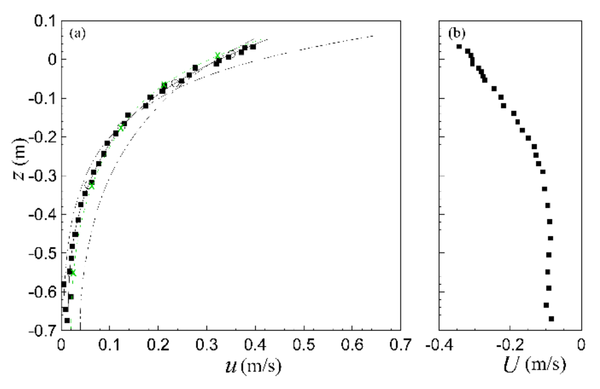
4.3. Non-Linear Wave Interacting with Depth-Varying Current

We further show the FNHS/QNHS pressure effects on nonlinear wave interacting with a depth-varying current [11]. Based upon the experimental configuration, the numerical tank has a length of 20 m and an undisturbed water depth of 0.7 m. The conditions of incident wave (period T and height H) and measured profiles of following/opposing current (surface velocity U_s and surface vorticity ω_s) are specified according to case 5 (T = 0.75 s; H = 0.079 m; U_s = 0.42 m/s; ω_s = 2.09 s⁻¹) and case 10 (T = 1.0 s; H = 0.104 m; U_s = −0.348 m/s; ω_s = −0.89 s⁻¹). A grid spacing of Δx = 0.05 m and five stretched vertical layers are used to discretize the model domain. The time-step is determined by setting Cr = 0.1.

4.3.1. Interaction with a Negatively Sheared Opposing Current

Figure 15 presents the measured current profile U(z) and compares the predictions of wave-induced velocity u(z) under wave crest. In addition to the experimental data, the fifth-order wave-only and Doppler-shifted solutions (respectively for U(z) = 0 and U(z) = U_s) are also included [5]. Compared with the wave-only solution, the Doppler-shifted results have a larger surface velocity with a shaper distribution along the depth owing to the enlarged amplitude and shortened wavelength/increased dimensionless water depth Kh [64]. For the sheared current, the presence of vorticity at the upper depth (−0.25 m < z < 0 m) counteracts the Doppler shift by the surface current U_s [65] and then yields the smaller velocity as observed in the experiments. The FNHS results and observation data are in excellent agreement. The QNHS results appear to capture the structure of horizontal velocity as the convective effects are diminished, possibly by the opposing current.

4.3.2. Interaction with a Positively Sheared Following Current

Similar comparisons in Figure 16 show the contrary results in case 5. The Doppler shift by a positively uniform current presents a smaller surface velocity with a milder vertical distribution because of the decreased amplitude and lengthened wavelength (lessened dimensionless depth Kh). The vorticity of the sheared current moderates the shift, giving the larger velocity for the upper depth (i.e., −0.25 m < z < 0 m). The FNHS simulation exactly resolves the horizontal velocity profile, similar to the five-layered model results in [11]. Close to the Doppler-shifted solution, the QNHS simulation without convective vertical acceleration fails to represent the interaction of non-linear waves with the strongly sheared following current. Apparently, the wave-induced velocity with a noticeable (i.e., 20%) under-estimation near the surface can be found. Overall, the inter-comparison clearly reveals the fully non-hydrostatic effects on complicated wave–current interactions.

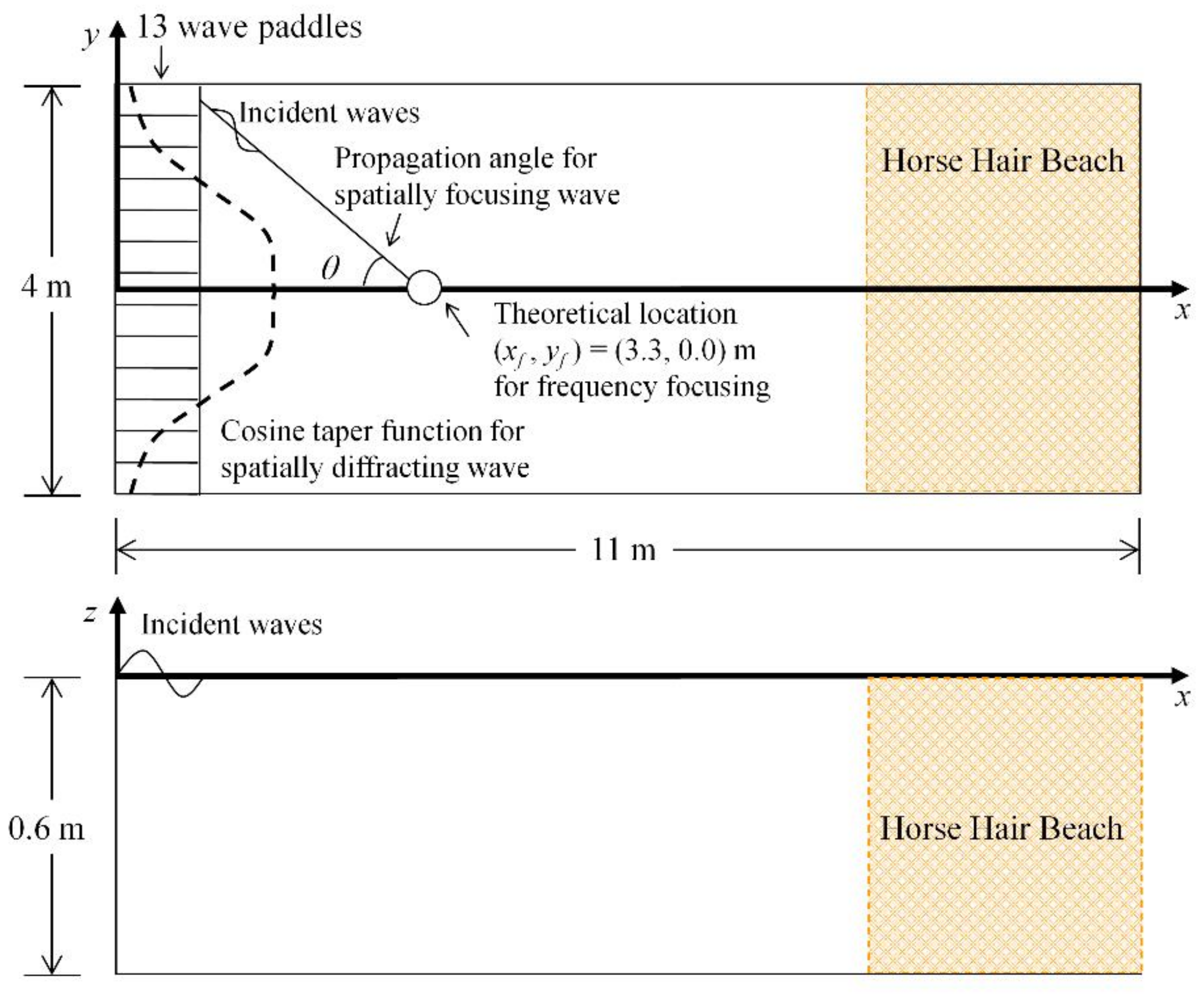
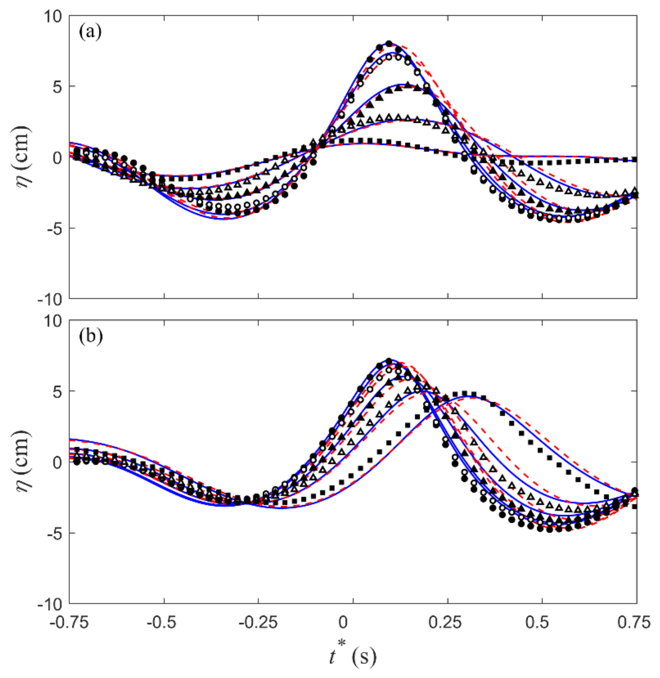
4.4. Spatial Focusing and Diffracting Waves

Lastly, we explore the FNHS/QNHS pressure effects upon the propagation of directional waves, that is, the spatial focusing and diffracting waves in the deep water [66]. In these two cases, a three-dimensional version of the non-hydrostatic model [49] is employed. The numerical wave flume (see Figure 17) has a length of 11 m, a width of 4 m, and an undisturbed mean water depth of h = 0.6 m, according to the experimental configuration. A deep-water spectral wave group with 32 components ranging from f = 0.6855 to 1.4745 Hz (or Kh = 1.311 to 5.246) are considered. The incident waves are generated based upon the frequency focusing technique with an addition of directionality. For the spatial focusing waves, the motion of each wave paddle is prescribed by the horizontal velocity, that is,

$$u(x=0,y=y_p,z,t)={\displaystyle \sum _{n=1}^{N=32}{a}_n{\omega }_n\frac{\cosh [K_n(h+z)]}{\sinh (K_{n}h)}}\cos [-K_n\cos {\theta }_p{x}_f-K_n\sin {\theta }_p\left|y_p\right|-{\omega }_n(t-t_f)]\cos {\theta }_p$$

(9)

where the amplitude a_n is chosen to produce a constant steepness spectrum; ω_n and K_n are the angular frequency and wave number of the nth component; the incident angle of each paddle is θ_p = tan⁻¹(x_f/|y_p|); the theoretical focusing location x_f =3.3 m, and time t_f =12 s are set. For the spatial diffracting waves, a lateral variation from |y_p| = 0.45 m to |y_p| = 2 m is introduced into the horizontal velocity using a cosine window that tapers the amplitude down to 10% at the lateral boundaries, that is,

$$u(x=0,y=y_p,z,t)={\displaystyle \sum _{n=1}^{N=32}{a}_n{\omega }_n\frac{\cosh [K_n(h+z)]}{\sinh (K_{n}h)}}\cos [-K_n{x}_f-{\omega }_n(t-t_f)][0.1+0.9{\cos }^2\frac{\left|y_p\right|\pi }{4}]$$

(10)

Here, we choose the non-breaking incipient conditions (i.e., a_nk_n = 0.0055). At the outgoing boundary, a 3 m long sponge layer in conjunction with the Sommerfield radiation boundary condition is applied to minimize wave reflection. The computational domain is horizontally discretized by a set of uniform cells with the spatial increment Δx = Δy = 0.05 m. In the vertical direction, five layers are used to cover the full spectral range evolution. The model is run for the total simulation time 40 s, with a small time-step Δt = 0.001 s.

4.4.1. Spatial Focusing Waves

The spatial focusing waves have been regarded as an important formation mechanism of the so-called oceanic freak waves that can mysteriously occur and cause notorious hazards. Figure 18a shows the perspective view of the FNHS modeled wave field in the vicinity of the focusing event. As clearly found in the progress of wave evolution, a “hole in the sea” is followed by the “wall of waters” during t^∗ = −1 s to −0.5 s, presenting an exceptionally large, steep, and asymmetric wave. At the consecutive stage (i.e., at t^∗ = 0 s), an extreme freak wave is rapidly developed with a maximum amplitude twice over the average wave height of the wave packet, which is the main characteristic of freak waves [67]. Afterward, the freak wave disappears in a second (t^∗ = 1 s), consistent with the short-live feature reported by field observations [68]. Note that owing to nonlinearity, the actual focusing event does not occur at the theoretical location prescribed by the linear theory [66]. Figure 19a compares the FNHS/QNHS model results of free-surface elevation time-series with the available recorded data at x = x_f = 3.3 m and different lateral locations, i.e., y = 0, 0.3, 0.6, 0.9, and 1.5 m. The FNHS model well predicts the distinctive crescent shape of the wave crest. The FNHS (or QNHS) predicted focusing event yields a maximum wave crest of 8.04 cm (or 7.94 cm). The actual focusing locations from both computations give a small deviation of 0.05 m (a grid spacing size), that is, a slightly shorter focusing distance in QNHS. Interestingly, the FNHS/QNHS results reveal insignificant differences for the fast-modulated focusing waves, in contrast to the slowly modulated, nonlinear, bi-chromatic wave train. Reasonable explanation might be the weaker wave–wave interactions between each smaller steepness wave component (i.e., a_nk_n = 0.0055) in this nonlinear transient phenomenon.

4.4.2. Spatial Diffracting Waves

The spatial diffracting waves can be used to represent those waves in an actual field condition with small-scale heterogeneity in amplitude due to inhomogeneous winds. Similarly, Figure 18b shows the perspective view of the developing wave field modeled by the FNHS condition. One can clearly see that the wave front diffracts as it evolves to an extreme event through frequency focusing. Figure 19b further compares the FNHS/QNHS simulated free-surface elevation time-series with the experimental data. Due to different directionality, the spatial diffracting wave crest is crescent-shaped, but with an obvious centerline leading. The FNHS- and QNHS-predicted extreme events respectively yield maximum wave crests of 7.84 cm and 7.71 cm, with a 0.05 m difference in the actual locations. The FNHS and QNHS model results are quite close, consistent with the finding and explanation in spatial focusing waves. Here, the wave–wave interactions in the incipient focusing and diffracting waves are not as strong as those in the nonlinear bi-chromatic waves, while such a physical process is greatly affected by the FNHS/QNHS pressure conditions. Overall, wave directionality does not strongly interfere with the FNHS/QNHS pressure effects on the evolution of directional waves.

5. Summary and Conclusions

Surface water waves with significant influences upon human activities is an important research topic in the field of coastal and ocean engineering [1,2,3]. In this study, a high-order NHS model [49,51] was used to gain a deeper insight for the effects of non-hydrostatic pressure on surface wave motions and its role in numerical modeling. First, relative contribution of non-hydrostatic pressure P_nhs/P_hs and its effects (sensitivity) on wave celerity and amplitude were carefully evaluated. For linear wave dispersion [1], non-hydrostatic pressure contributed from the local vertical acceleration, confirmed by the identical FNHS and QNHS results. The vertical structure of P_nhs/P_hs clearly indicated stronger NHS effects in deeper waters and its significance near the surface. Overall, the NHS effects would slow-down wave celerity, but remain the incident amplitude for the deep-water waves, compared to the unrealistic long-wave patterns in the HS results. The sensitivity could also be easily described by the pressure and celerity errors (e.g., ε_p = 3% and ε_c = 6% (at Kh = 20)). In terms of wave non-linearity [5], non-hydrostatic pressure revealed similar features, except a larger magnitude and different surface contribution pattern. Non-hydrostatic pressure components caused by the convective vertical acceleration was responsible for the increased amplitude and phase speed under strong non-linearity.

The FNHS/QNHS model [49,51] was then applied to investigate the effects of non-hydrostatic pressure for waves involving complicated interactions (i.e., wave, bottom, and current, as well as directionality). In the bi-chromatic deep-water wave train [9], the FNHS results predict the modulation of non-linear wave groups. Without convective vertical acceleration, the QNHS simulation could not capture side-band frequencies, giving the unrealistic phase speed (or group velocity) and amplitude. For the non-linear wave shoaling example [18], the FNHS results resolve the wave transformation and the QNHS predictions under-estimated wave amplitude and celerity. In terms of wave–current interactions [11], both of the FNHS and QNHS results reasonably describe wave-induced velocity under a negatively sheared opposing current, possibly due to the diminished convective effects. However, unlike the good agreement between the FNHS results and experimental data, the QNHS prediction (similar to the Doppler-shifted solution) was incapable of handling non-linear wave interaction with a strongly sheared following current. Lastly, wave directionality did not strongly interfere with the FNHS/QNHS effects on the evolution of spatial focusing and diffracting waves [66]. The FNHS and QNHS model results are quite close, possibly due to much weaker wave–wave interactions. Overall, the non-hydrostatic effects on wave propagation/transformation and its role in nonlinear dispersive wave modeling have been clearly elucidated.

References

1. Mei, C.C.; Liu, P.L.F. Surface waves and coastal dynamics. Annu. Rev. Fluid Mech. 1993, 25, 215–240. [Google Scholar] [CrossRef]
2. Battjes, J.A. Developments in coastal engineering research. Coast. Eng. 2006, 23, 121–132. [Google Scholar] [CrossRef]
3. Cavaleri, L.; Alves, J.H.G.M.; Ardhuin, F.; Babanin, A.; Banner, M.; Belibassakis, K.; Benoit, M.; Donelan, M.; Groeneweg, J.; Herbers, T.H.C.; et al. Wave modelling—The state of the art. Prog. Oceanogr. 2007, 75, 603–674. [Google Scholar] [CrossRef] [Green Version]
4. Mei, C.C. The Applied Dynamics of Ocean Surface Waves; Wiley Inter-Science: New York, NY, USA, 1983. [Google Scholar]
5. Fenton, J.D. A fifth-order Stokes theory for steady waves. J. Waterw. Port Coast. Ocean Eng. 1985, 111, 216–234. [Google Scholar] [CrossRef] [Green Version]
6. Beji, S.; Battjes, J.A. Experimental investigation of wave propagation over a bar. Coast. Eng. 1993, 19, 151–162. [Google Scholar] [CrossRef]
7. Melville, W.K. The instability and breaking of deep-waterwaves. J. Fluid Mech. 1982, 115, 165–185. [Google Scholar] [CrossRef] [Green Version]
8. Kirby, J.T. Nonlinear, dispersive long waves in water of variable depth. In Gravity Waves in Water of Finite Depth; Advances in Fluid Mechanics, Series; Hunt, J.N., Ed.; Computational Mechanics Publications: Southampton, UK, 1997; Volume 10, pp. 55–125. [Google Scholar]
9. Hwung, H.H.; Chiang, W.S. The measurements on wave modulation and breaking. Meas. Sci. Technol. 2005, 16, 1921–1928. [Google Scholar] [CrossRef]
10. Ting, C.L.; Chao, W.T.; Young, C.C. Experimental investigation of nonlinear regular wave transformation over a submerged step: Harmonic generation and wave height modulation. Coast. Eng. 2016, 117, 19–31. [Google Scholar] [CrossRef]
11. Swan, C.; Cummins, I.P.; James, R.L. An experimental study of two-dimensional surface water waves propagating on depth-varying currents. Part 1. Regular waves. J. Fluid Mech. 2001, 428, 273–304. [Google Scholar] [CrossRef]
12. Yao, A.F.; Wu, C.H. Spatial and temporal characteristics of transient extreme wave profiles on depth-varying currents. J. Eng. Mech. 2006, 132, 1015–1025. [Google Scholar] [CrossRef]
13. Tsai, W.T.; Yue, D.K.P. Computation of nonlinear free-surface flows. Annu. Rev. Fluid Mech. 1996, 28, 249–278. [Google Scholar] [CrossRef]
14. Liu, P.L.F.; Losada, I.J. Wave propagation modeling in coastal engineering. J. Hydraul. Res. 2002, 40, 229–240. [Google Scholar] [CrossRef]
15. Choi, D.Y.; Wu, C.H. A new efficient 3D non-hydrostatic free-surface flow model for simulating water wave motions. Ocean Eng. 2006, 33, 587–609. [Google Scholar] [CrossRef]
16. Peregrine, D.H. Long waves on a beach. J. Fluid Mech. 1967, 27, 815–827. [Google Scholar] [CrossRef]
17. Madsen, P.A.; Sørensen, O.R. A new form of the Boussinesq equations with improved linear dispersion characteristics. Part 2. A slowly-varying bathymetry. Coast. Eng. 1992, 18, 183–204. [Google Scholar] [CrossRef]
18. Nwogu, O. Alternative form of Boussinesq equations for nearshore wave propagation. J. Waterw. Port Coast. Ocean Eng. 1993, 119, 618–638. [Google Scholar] [CrossRef] [Green Version]
19. Gobbi, M.F.; Kirby, J.T.; Wei, G. A fully nonlinear Boussinesq model for surface waves. II. Extension to O((kh)4). J. Fluid Mech. 2000, 405, 182–210. [Google Scholar] [CrossRef] [Green Version]
20. Madsen, P.A.; Bingham, H.B.; Liu, H. A new Boussinesq method for fully nonlinear waves from shallow to deep water. J. Fluid Mech. 2002, 462, 1–30. [Google Scholar] [CrossRef]
21. Lynett, P.; Liu, P.L.F. A two-layer approach to wave modeling. Proc. Math. Phys. Eng. Sci. 2004, 460, 2637–32669. [Google Scholar] [CrossRef]
22. Berkhoff, J.C.W. 1972 Computation of combined refraction—Diffraction. In Proceedings of the 13th International Conference on Coastal Engineering, Vancouver, BC, Canada, 10–14 July 1972; pp. 471–490. [Google Scholar]
23. Nadaoka, K.; Beji, S.; Nakagawa, Y. A fully dispersive weakly nonlinear model for water waves. Proc. Math. Phys. Eng. Sci. 1997, 453, 303–318. [Google Scholar] [CrossRef]
24. Smith, R.A. An operator expansion formalism for nonlinear surface waves over variable depth. J. Fluid Mech. 1998, 363, 333–347. [Google Scholar] [CrossRef]
25. Longuet-Higgins, M.S.; Cokelet, E.D. The deformation of steep surface waves on water. I A numerical method of computation. Proc. Math. Phys. Eng. Sci. 1976, 95, 1–26. [Google Scholar]
26. Dold, J.W.; Peregrine, D.H. Steep unsteady waves: An efficient computational scheme. In Proceedings of the 19th International Conference on Coastal Engineering, Houston, TX, USA, 3–7 September 1984; pp. 955–967. [Google Scholar]
27. Ohyama, T.; Nadaoka, K. Development of a numerical wave tank for analysis of nonlinear and irregular wave field. Fluid Dyn. Res. 1991, 8, 231–251. [Google Scholar] [CrossRef]
28. Li, B.; Fleming, C.A. A three dimensional multigrid model for fully nonlinear water waves. Coast. Eng. 1997, 30, 235–258. [Google Scholar] [CrossRef]
29. Turnbull, M.S.; Borthwick, A.G.L.; Eatock Taylor, R. Numerical wave tank based on a σ-transformed finite element inviscid flow solver. Int. J. Numer. Methods Fluids 2003, 42, 641–663. [Google Scholar] [CrossRef]
30. Guyenne, P.; Grilli, S.T. Numerical study of three-dimensional overturning waves in shallow water. J. Fluid Mech. 2006, 547, 361–388. [Google Scholar] [CrossRef] [Green Version]
31. Mayer, S.; Garapon, A.; Sørensen, L.S. A fractional step method for unsteady free-surface flow with applications to non-linear wave dynamics. Int. J. Numer. Methods Fluids 1998, 28, 293–315. [Google Scholar] [CrossRef]
32. Casulli, V. A semi-implicit finite difference method for non-hydrostatic, free-surface flows. Int. J. Numer. Methods Fluids 1999, 30, 425–440. [Google Scholar] [CrossRef]
33. Li, B.; Fleming, C.A. Three-dimensional model of Navier-Stokes equations for water waves. J. Waterw. Port Coast. Ocean Eng. 2001, 127, 16–25. [Google Scholar] [CrossRef]
34. Namin, M.M.; Lin, B.; Falconer, R. An implicit numerical algorithm for solving non-hydrostatic free-surface flow problems. Int. J. Numer. Methods Fluids 2001, 35, 341–356. [Google Scholar] [CrossRef]
35. Kocyigit, M.B.; Falconer, R.A.; Lin, B. Three-dimensional numerical modeling of free surface flows with non-hydrostatic pressure. Int. J. Numer. Methods Fluids 2002, 40, 1145–1162. [Google Scholar] [CrossRef]
36. Chen, X. A fully hydrodynamic model for three-dimensional, free-surface flows. Int. J. Numer. Methods Fluids 2003, 42, 929–952. [Google Scholar] [CrossRef]
37. Hsu, T.J.; Liu, P.L.F. Toward modeling turbulent suspension of sand in the nearshore. J. Geophys. Res. Oceans 2004, 109, C06018. [Google Scholar] [CrossRef] [Green Version]
38. Wu, C.H.; Young, C.C.; Chen, Q.; Lynett, P.J. Efficient non-hydrostatic modeling of nonlinear waves from shallow to deep water. J. Waterw. Port Coast. Ocean Eng. 2010, 136, 104–118. [Google Scholar] [CrossRef]
39. Ma, G.; Shi, F.; Kirby, J.T. Shock-capturing non-hydrostatic model for fully dispersive surface wave processes. Ocean Model. 2012, 43, 22–35. [Google Scholar] [CrossRef]
40. Bai, Y.; Cheung, K.F. Dispersion and nonlinearity of multi-layer non-hydrostatic free-surface flow. J. Fluid Mech. 2013, 726, 226–260. [Google Scholar] [CrossRef]
41. Stelling, G.; Zijlema, M. An accurate and efficient finite-difference algorithm for non-hydrostatic free-surface flow with application to wave propagation. Int. J. Numer. Methods Fluids 2003, 43, 1–23. [Google Scholar] [CrossRef]
42. Zijlema, M.; Stelling, G. Further experiences with computing non-hydrostatic free-surface flows involving water waves. Int. J. Numer. Methods Fluids 2005, 48, 169–197. [Google Scholar] [CrossRef]
43. Yuan, H.; Wu, C.H. An implicit 3D fully non-hydrostatic model for free-surface flows. Int. J. Numer. Methods Fluids 2004, 46, 709–733. [Google Scholar] [CrossRef]
44. Yuan, H.; Wu, C.H. A two-dimensional vertical non-hydrostatic σ model with an implicit method for free-surface flows. Int. J. Numer. Methods Fluids 2004, 44, 811–835. [Google Scholar] [CrossRef]
45. Yuan, H.; Wu, C.H. Fully Nonhydrostatic Modeling of Surface Waves. J. Eng. Mech. 2006, 132, 447–456. [Google Scholar] [CrossRef]
46. Ahmadi, A.; Badiei, P.; Namin, M.M. An implicit two-dimensional non-hydrostatic model for free-surface flows. Int. J. Numer. Methods Fluids 2007, 54, 1055–1074. [Google Scholar] [CrossRef]
47. Badiei, P.; Namin, M.M.; Ahmadi, A. A three-dimensional non-hydrostatic vertical boundary fitted model for free-surface flows. Int. J. Numer. Methods Fluids 2008, 56, 607–627. [Google Scholar] [CrossRef]
48. Young, C.C.; Wu, C.H.; Kuo, J.T.; Liu, W.C. A higher-order σ-coordinate non-hydrostatic model for nonlinear surface waves. Ocean Eng. 2007, 34, 1357–1370. [Google Scholar] [CrossRef]
49. Young, C.C.; Wu, C.H.; Liu, W.C.; Kuo, J.T. A higher-order non-hydrostatic s model for simulating non-linear refraction-diffraction of water waves. Coast. Eng. 2009, 56, 919–930. [Google Scholar] [CrossRef]
50. Young, C.C.; Wu, C.H. An efficient and accurate non-hydrostatic model with embedded Boussinesq-type like equations for surface wave modeling. Int. J. Numer. Methods Fluids 2009, 60, 27–53. [Google Scholar] [CrossRef]
51. Young, C.C.; Wu, C.H. Nonhydrostatic Modeling of Nonlinear Deep-Water Wave Groups. J. Eng. Mech. 2010, 136, 155–167. [Google Scholar] [CrossRef]
52. Choi, D.Y.; Wu, C.H.; Young, C.C. An efficient curvilinear non-hydrostatic model for simulating surface water waves. Int. J. Numer. Methods Fluids 2011, 66, 1093–1115. [Google Scholar] [CrossRef]
53. Young, C.C.; Chao, W.T.; Ting, C.L. Applicable sloping range and bottom smoothing treatment for σ-based modeling of wave propagation over rapidly varying topography. Ocean Eng. 2016, 125, 261–271. [Google Scholar] [CrossRef]
54. Chen, X. A comparison of hydrostatic and nonhydrostatic pressure components in seiche oscillations. Math. Comput. Model. 2005, 41, 887–902. [Google Scholar] [CrossRef]
55. Casulli, V.; Stelling, G.S. Numerical simulation of 3D quasi-hydrostatic free-surface flows. J. Hydraul. Eng. 1998, 124, 678–686. [Google Scholar] [CrossRef]
56. Bradford, S.F. Godunov-based model for nonhydrostatic wave dynamics. J. Waterw. Port Coast. Ocean Eng. 2005, 131, 226–238. [Google Scholar] [CrossRef]
57. Chiang, W.S.; Hsiao, S.C.; Hwung, H.H. Evolution of sidebands in deep-water bichromatic wave trains. J. Hydraul. Res. 2007, 45, 67–80. [Google Scholar] [CrossRef]
58. Trulsen, K.; Stansberg, C.T. Spatial evolution of water surface waves: Numerical simulation and experiment of bichromatic waves. In Proceedings of the Eleventh International Offshore and Polar Engineering Conference, Stavanger, Norway, 17–22 June 2001; International Society of Offshore and Polar Engineers: Mountain View, CA, USA, 2001. [Google Scholar]
59. Longuet-Higgins, M.S.; Stewart, R.W. Changes in the form of short gravity waves on long waves and tidal currents. J. Fluid Mech. 1960, 8, 565–583. [Google Scholar] [CrossRef]
60. Bateman, W.J.D.; Swan, C.; Taylor, P.H. On the efficient numerical simulation of directionally spread surface water waves. J. Comput. Phys. 2001, 174, 277–305. [Google Scholar] [CrossRef]
61. Shemer, L.; Jiao, H.; Kit, E.; Agnon, Y. Evolution of a nonlinear wave field along a tank: Experiments and numerical simulations based on the spatial Zakharov equation. J. Fluid Mech. 2001, 427, 107–129. [Google Scholar] [CrossRef] [Green Version]
62. Westhuis, J.; van Groesen, E.; Huijsmans, R. Experiments and numerics of bichromatic wave groups. J. Waterw. Port Coast. Ocean Eng. 2001, 127, 334–342. [Google Scholar] [CrossRef]
63. Ting, F.C.K.; Kirby, J.T. Observation of undertow and turbulence in a laboratory surf zone. Coast. Eng. 1994, 24, 51–80. [Google Scholar] [CrossRef]
64. Peregrine, D.H. Interaction of water waves and currents. Adv. Appl. Mech. 1976, 16, 9–117. [Google Scholar]
65. Nepf, H.; Monismith, S. Wave dispersion on a sheared current. Appl. Ocean Res. 1994, 16, 313–316. [Google Scholar] [CrossRef]
66. Wu, C.H.; Nepf, H.M. Breaking wave criteria and energy losses for three-dimensional wave breaking. J. Geophys. Res. Oceans 2002, 107, 3177. [Google Scholar] [CrossRef]
67. Dean, R.G. Freak waves: A possible explanation. In Water Wave Kinematics; Torum, O., Gudmestad, O.T., Eds.; Kluwer Academic Publishers: Dordrecht, The Netherlands, 1990; pp. 609–612. [Google Scholar]
68. Kharif, C.; Pelinovsky, E. Physical mechanisms of the rogue wave phenomenon. Eur. J. Mech. B Fluids 2003, 22, 603–634. [Google Scholar] [CrossRef] [Green Version]
Figure 1. Mesh transformation and staggered variable arrangement between (a) a Cartesian co-ordinate and (b) a σ co-ordinate system.
Water 12 03513 g001
Figure 2. Sketch of a vertical 2D numerical wave tank.
Water 12 03513 g002
Figure 3. (a) The vertical distribution of non-hydrostatic pressure and (b) the relative ratio between non-hydrostatic pressure and hydrostatic pressure under wave crest for linear dispersive waves: analytical solution (solid lines), FNHS (fully non-hydrostatic) mode (circles), QNHS (quasi non-hydrostatic) mode (X marks), and HS (hydrostatic) mode (triangles).
Water 12 03513 g003
Figure 4. Sensitivity analysis of the physical and modeled non-hydrostatic effects on the phase velocity of linear dispersive waves under different Kh: (a) wave speed and phase error εc and (b) non-hydrostatic contribution and pressure error εP at the top layer: analytical solution (bold solid lines) and FNHS mode (solid lines).
Water 12 03513 g004
Figure 5. Comparison of the predicted free-surface spatial profile for (a) Kh = π/25, (b) Kh = π/5, (c) Kh = π, and (d) Kh = 5π: analytical solution (solid lines), FNHS mode (circles), QNHS mode (X marks), and HS mode (triangles).
Water 12 03513 g005
Figure 6. (a) The vertical distribution of non-hydrostatic pressure and (b) the relative ratio between non-hydrostatic pressure and hydrostatic pressure under wave crest for non-linear deep-water waves: analytical solution (solid lines), FNHS mode (circles), and QNHS mode (X marks).
Water 12 03513 g006
Figure 7. Sensitivity analysis of the physical and modeled non-hydrostatic effects on the phase velocity of non-linear deep-water waves under different aK: (a) wave celerity and phase error εc and (b) non-hydrostatic contribution and pressure error εP at the top layer: analytical solution (bold solid lines), FNHS mode (solid lines), and QNHS mode (dashed lines).
Water 12 03513 g007
Figure 8. Comparison of the predicted free-surface displacement time series at x = 3λ for (a) aK= 0.10, (b) aK = 0.20, and (c) aK = 0.30: analytical solution (solid lines), FNHS mode (circles), and QNHS mode (X marks).
Water 12 03513 g008
Figure 9. The predicted free-surface displacement time series from the (a) FNHS results and (b) QNHS results for linear bi-chromatic waves: analytical solutions (circles), FNHS mode (solid lines), and QNHS mode (dashed lines).
Water 12 03513 g009
Figure 10. The predicted amplitude spectra from the (a) FNHS results and (b) QNHS results for linear bi-chromatic waves: analytical solutions (circles), FNHS mode (solid lines), and QNHS mode (dashed lines).
Water 12 03513 g010
Figure 11. Same as Figure 9, except for non-linear bi-chromatic waves (case B11): (a) FNHS results and (b) QNHS results.
Water 12 03513 g011
Figure 12. Same as Figure 10, except for non-linear bi-chromatic waves (case B11): (a) FNHS results and (b) QNHS results.
Water 12 03513 g012
Figure 13. (ac) The predicted spatial free-surface displacement for linear wave shoaling with Kh = 0.30, 3.13, and 9.0: wave envelope calculated by analytical solution (dashed lines), FNHS mode (solid lines), and QNHS mode (X marks). (d) The bottom configuration (bold solid lines) and the variation of Kh (dashed lines).
Water 12 03513 g013
Figure 14. (a) The spatial free-surface displacement from FNHS results (solid lines) for non-linear wave shoaling and the bottom configuration (bold solid lines). Comparison of the free-surface displacement time series at (b) station 1 and (c) station 2: experimental data (circles), FNHS mode (solid lines), and QNHS mode (dashed lines).
Water 12 03513 g014
Figure 15. (a) The vertical distribution of horizontal velocity and (b) measured current profile for non-linear waves interacting with negatively sheared opposing current: experimental data (squares), FNHS mode (solid lines with circles), QNHS mode (dashed lines with X marks), the wave-only solution (dash-dotted lines), and the Doppler-shifted solution (dash-dot-dotted lines).
Water 12 03513 g015
Figure 16. (a) The vertical distribution of horizontal velocity and (b) measured current profile for non-linear waves interacting with positively sheared following current: experimental data (squares), FNHS mode (solid lines with circles), QNHS mode (dashed lines with X marks), the wave-only solution (dash-dotted lines), and the Doppler-shifted solution (dash-dot-dotted lines).
Water 12 03513 g016
Figure 17. Sketch of the experimental setup by Wu and Nepf [66].
Water 12 03513 g017
Figure 18. Perspective views of the 3D spatially (a) focusing and (b) diffracting waves modeled with the FNHS mode.
Water 12 03513 g018
Figure 19. Comparison of the predicted free-surface displacement time series along lateral direction, that is, y = 0 m (filled circles), 0.3 m (open circles), 0.6 m (filled triangles), 0.9 m (open triangles), and 1.5 m (filled squares) for 3D spatially (a) focusing and (b) diffracting waves: experimental data (symbols), FNHS mode (solid lines), and QNHS mode (dashed lines).
Water 12 03513 g019
Publisher’s Note: MDPI stays neutral with regard to jurisdictional claims in published maps and institutional affiliations.