Effect of Independent Variables on Urban Flood Models


Abstract
1. Introduction
2. Materials and Methods
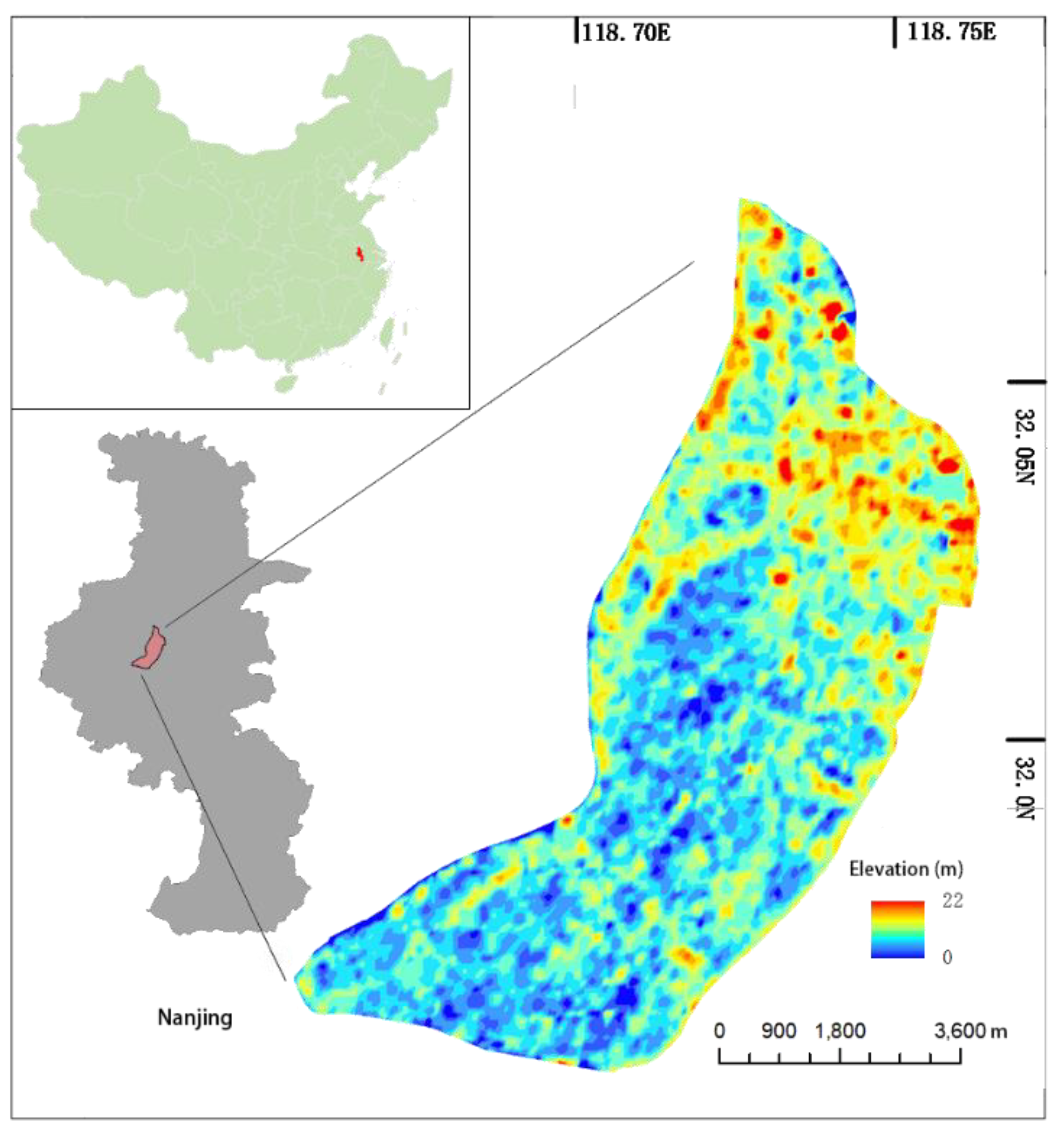
2.1. Study Area
2.2. Methods
2.2.1. Accuracy Evaluation
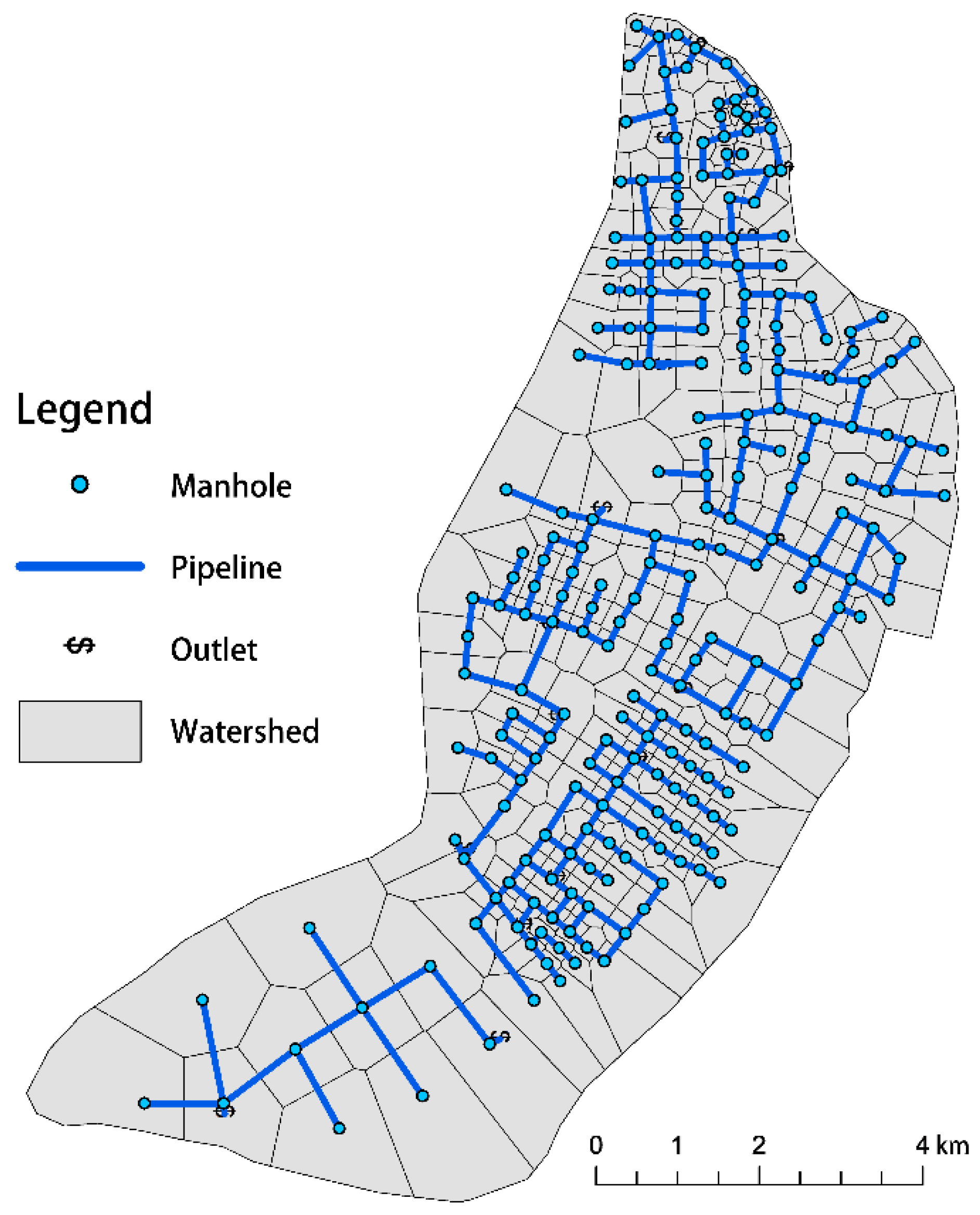
2.2.2. Hydraulic Model
3. Model Verification
4. Results and Discussion
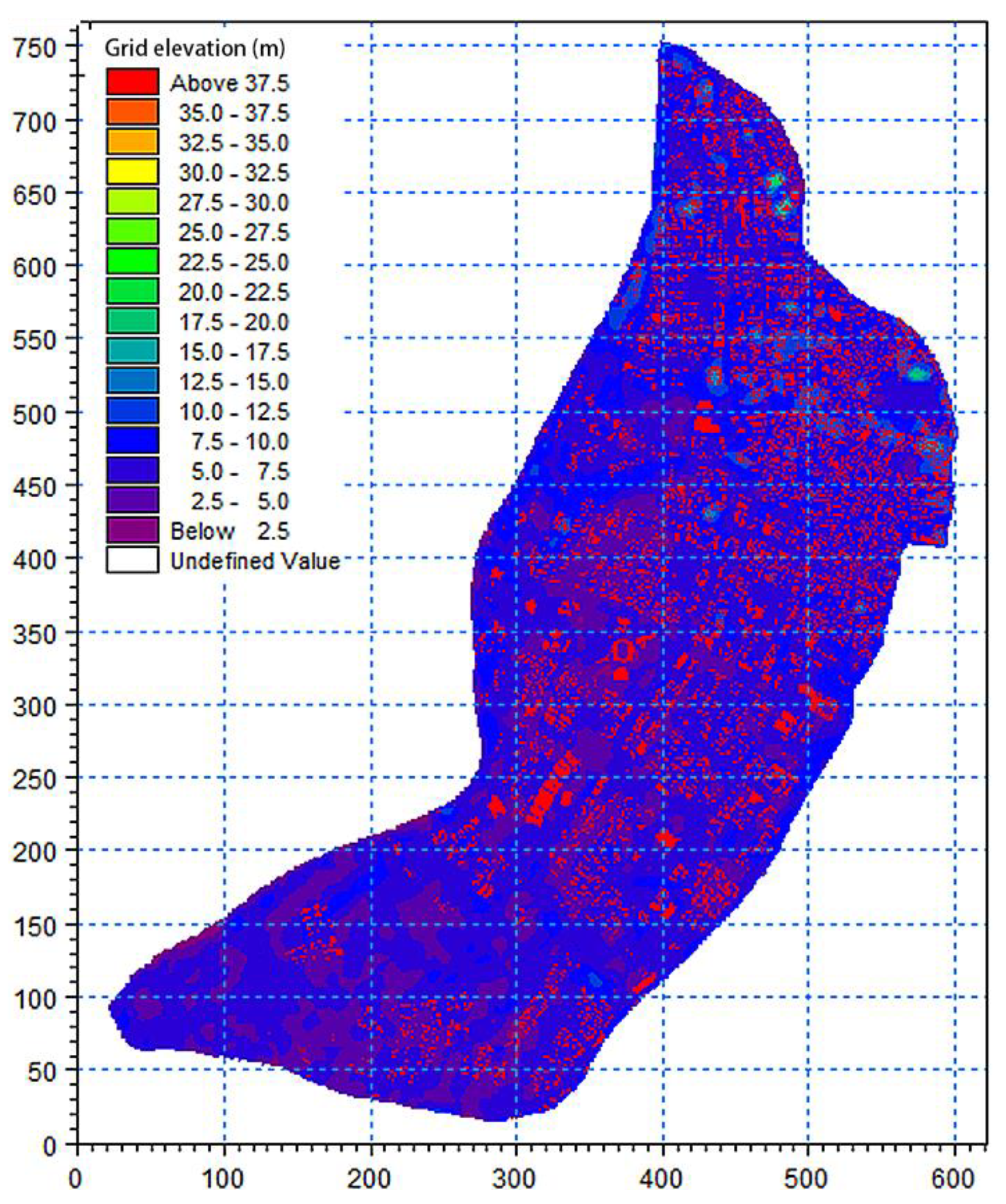
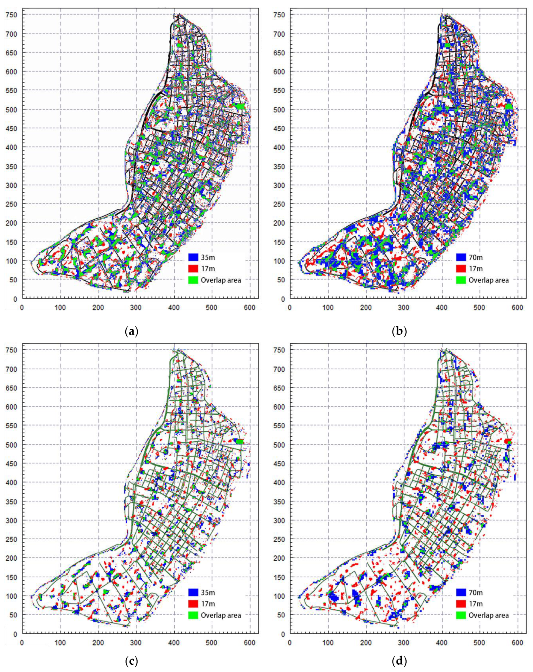
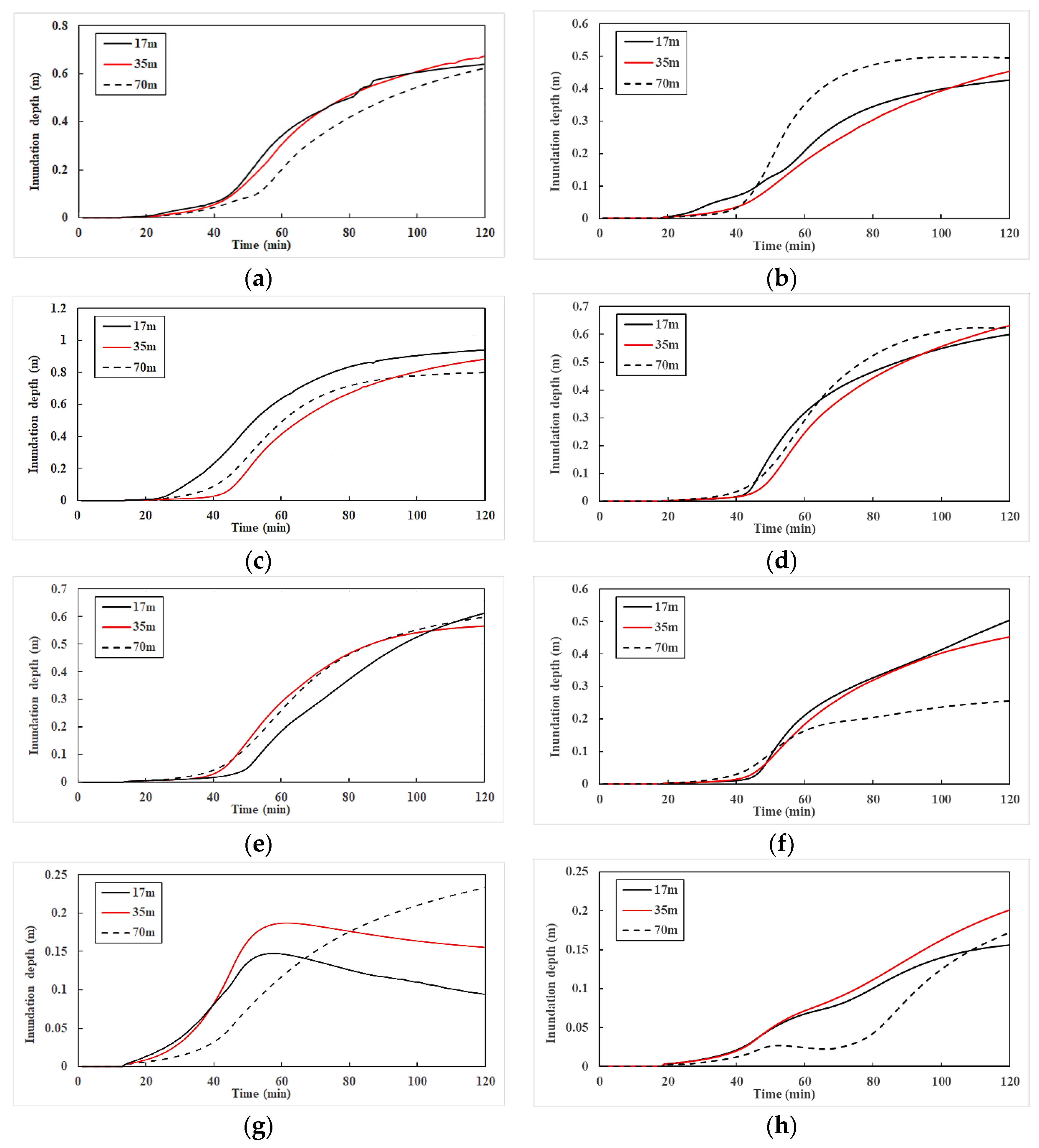
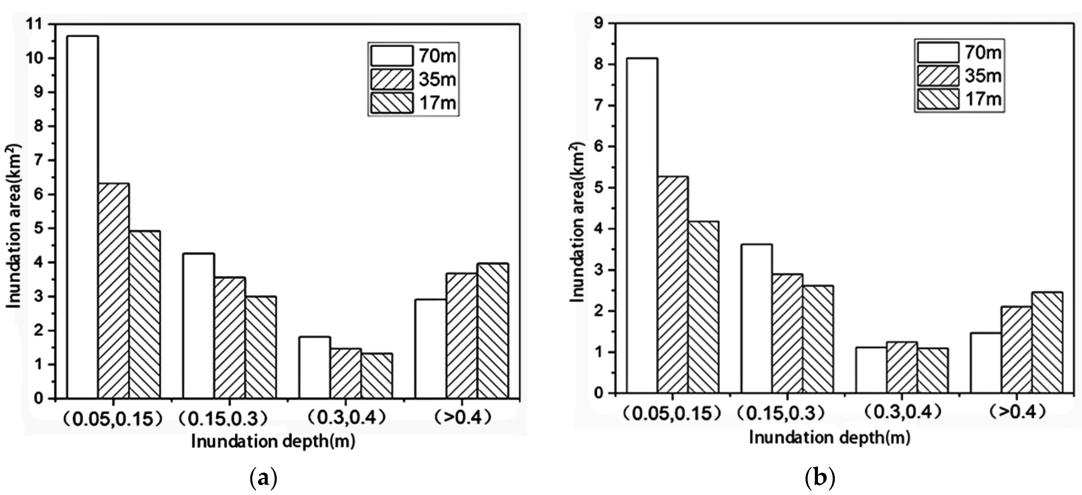
4.1. Terrain Resolution Simulation Analysis
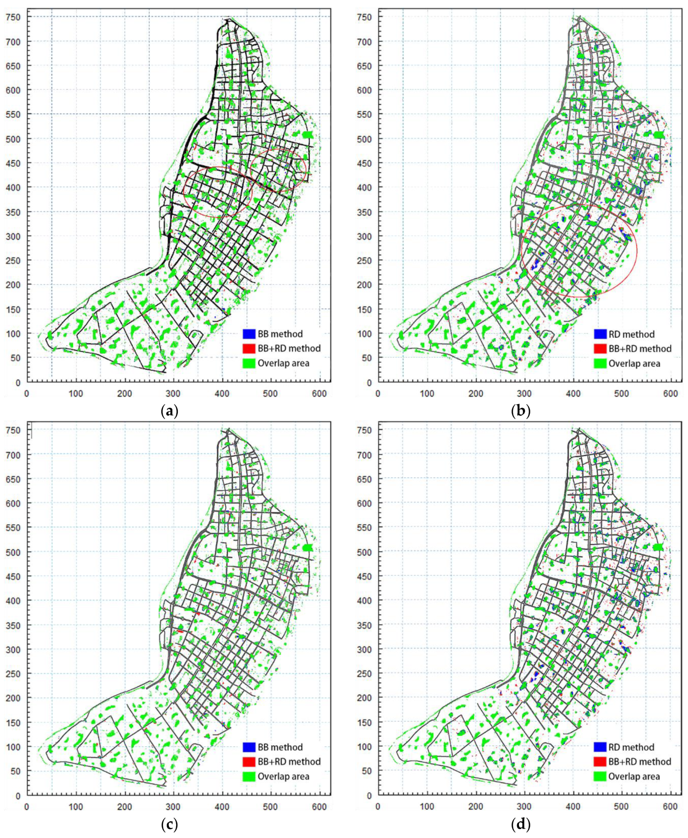
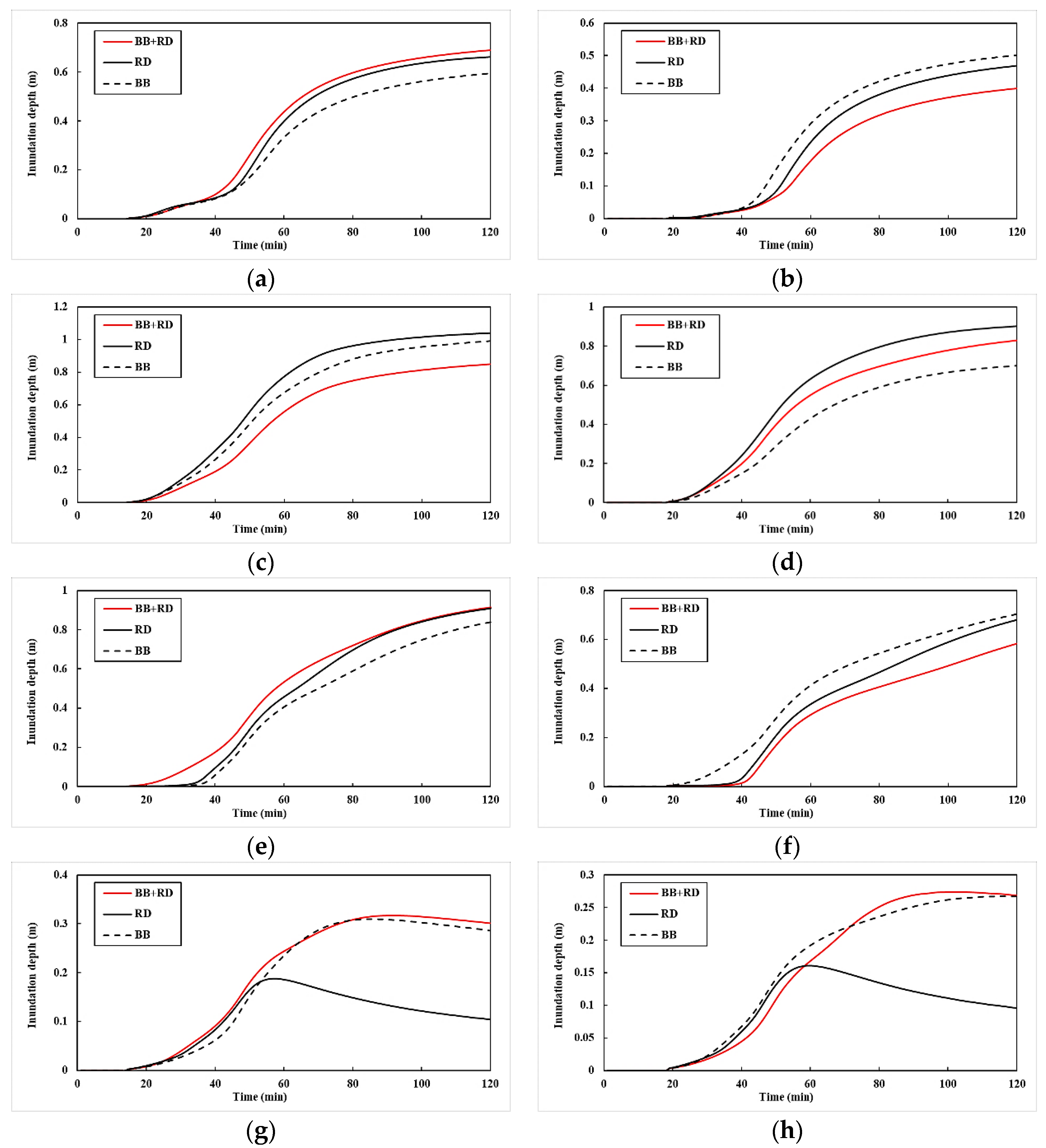
4.2. Artifical Land Cover Simulation Analysis
4.3. Comparative Analysis of All Simulation Schemes
5. Conclusions
- (1)
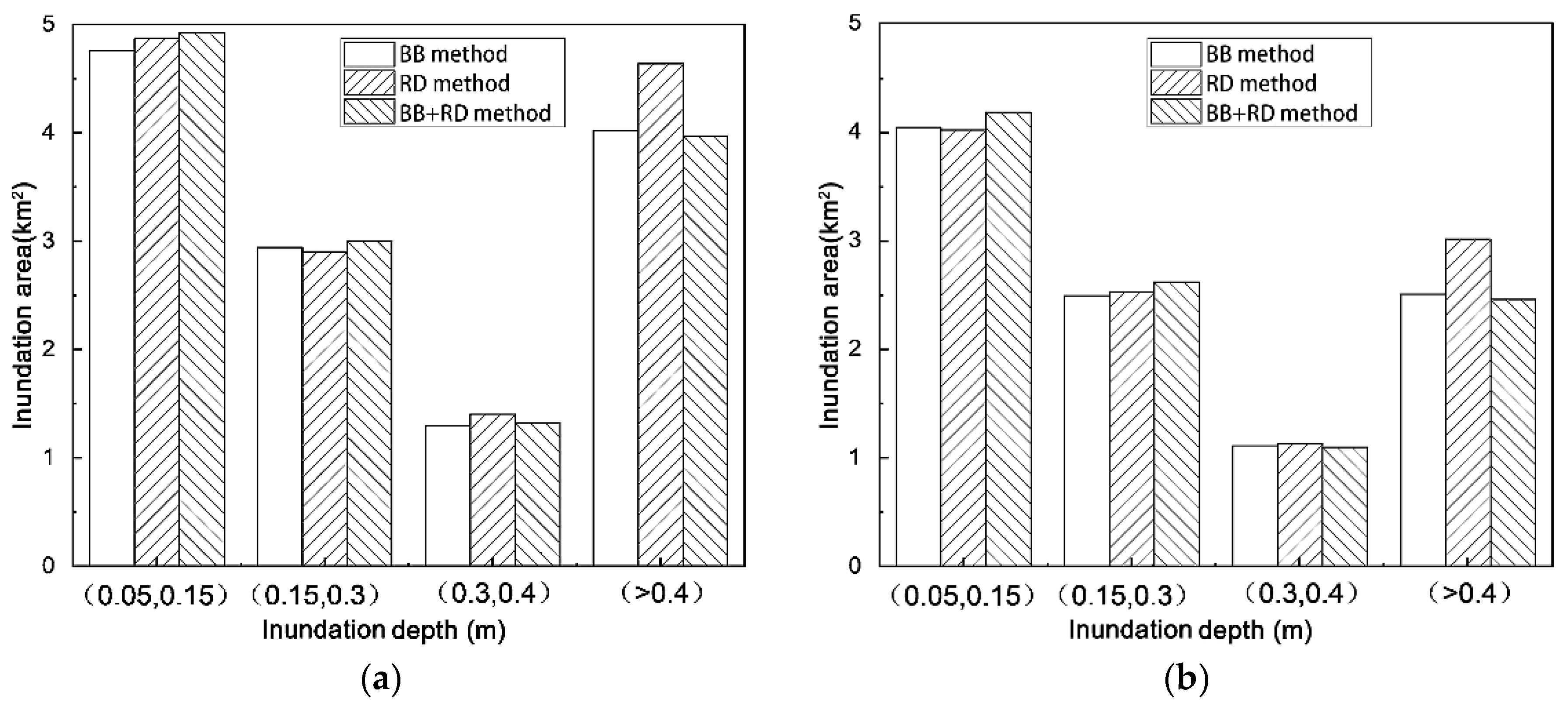
- The 35 m terrain resolution presented good accuracy in terms of the distribution of inundation area and flood evolution. Compared with the 70 m resolution, the error obtained for total inundation area was reduced by about 30% when using the 35 m resolution.
- (2)
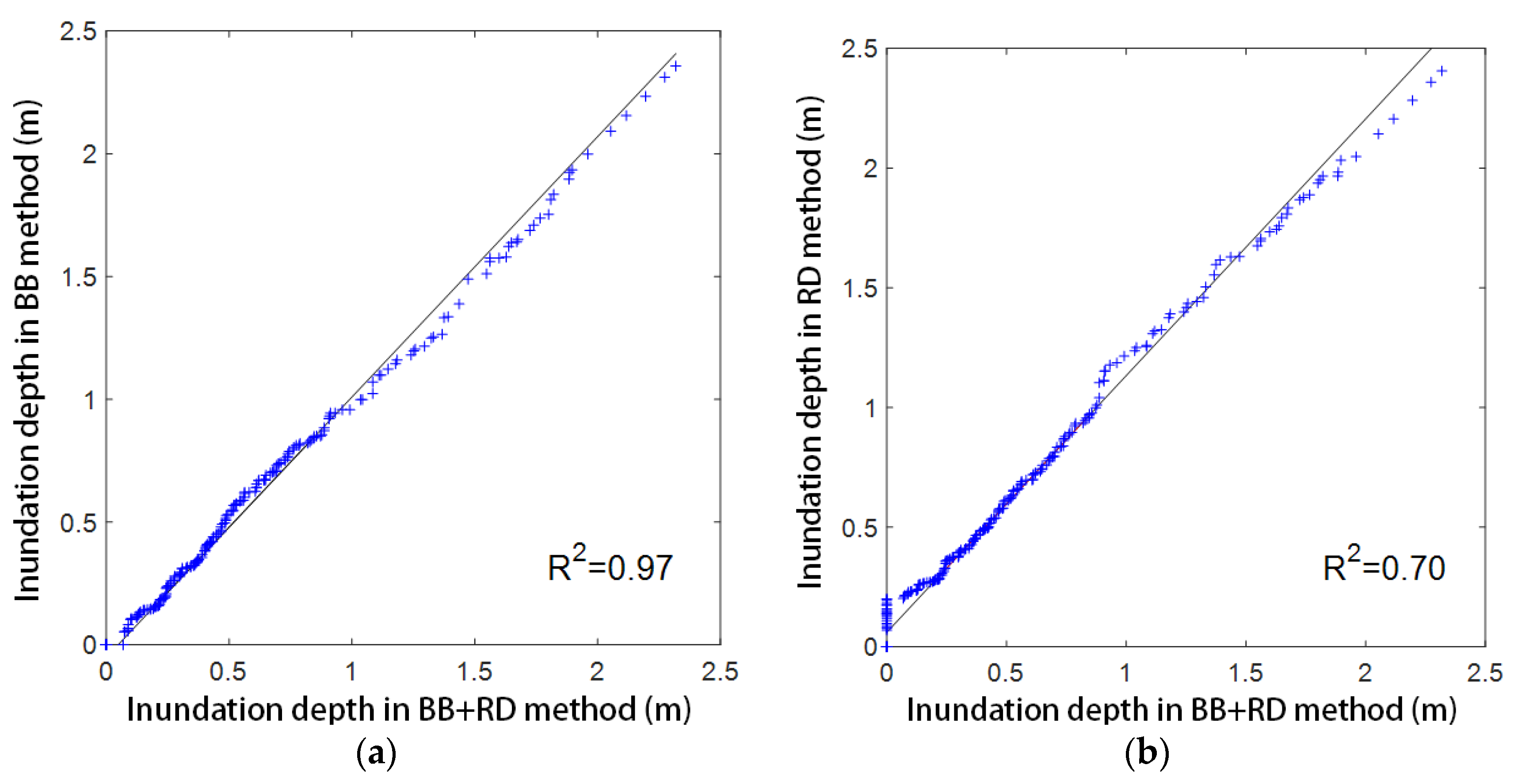
- In terms of representation methods of artificial land cover, the urban flood model using the BB method could better reflect the actual flood evolution than that using the RD method. Compared with the RD method, the correlation (R2) of the maximum inundation depth increased by about 30% when using the BB method.
- (3)
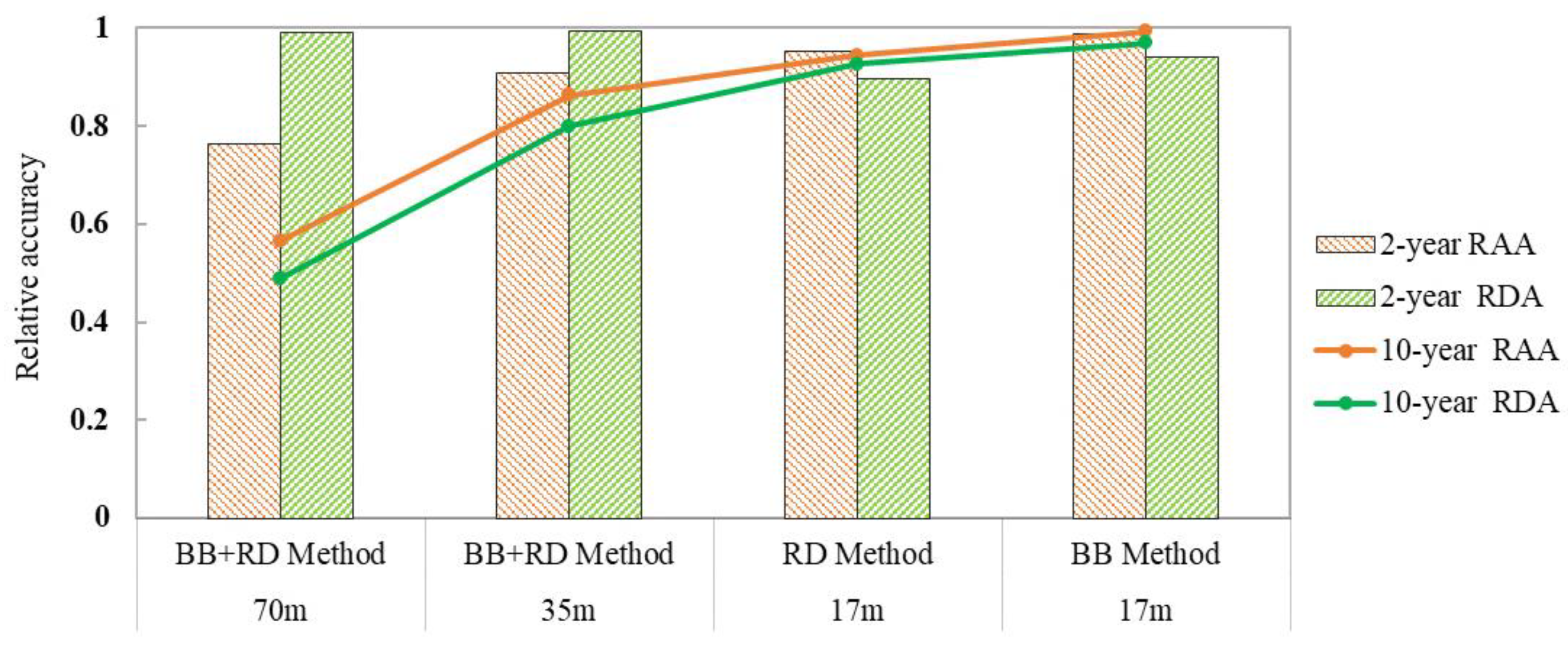
- The effect of terrain resolution on simulation accuracy was more obvious than that of artificial land cover. In the models using the BB + RD method, values of RAA and RDA could reach above 80% for the 35 m resolution models (20–30% higher than the 70 m terrain resolution models). In the models using the 17 m terrain resolution, values of RAA and RDA could reach above 94% when considering only the effect of buildings (5% higher than models only considering the effect of roads).
Author Contributions
Funding
Conflicts of Interest
References
- NDRCC, UNDP. Investigation Report on Risk Management Capability of Urban Flood Disaster; UNDP: New York, NY, USA, 2017. [Google Scholar]
- Mignot, E.; Li, X.; Dewals, B. Experimental Modelling of Urban Flooding: A Review. J. Hydrol. 2019, 568, 334–342. [Google Scholar] [CrossRef]
- Ahn, J.; Na, Y.; Park, S.W. Development of Two-Dimensional Inundation Modelling Process Using MIKE21 Model. KSCE J. Civ. Eng. 2019, 23, 3968–3977. [Google Scholar] [CrossRef]
- Geng, Y. Flood Risk Assessment in Quzhou City (China) Using a Coupled Hydrodynamic Model and Fuzzy Comprehensive Evaluation (FCE). Nat. Hazards 2020, 100, 133–149. [Google Scholar] [CrossRef]
- Zhang, W.; Zhang, X.; Liu, Y.; Tang, W.; Xu, J.; Fu, Z. Assessment of Flood Inundation by Coupled 1D/2D Hydrodynamic Modeling: A Case Study in Mountainous Watersheds along the Coast of Southeast China. Water 2020, 12, 822. [Google Scholar] [CrossRef]
- Viero, D.P. Modelling Urban Floods Using a Finite Element Staggered Scheme with an Anisotropic Dual Porosity Model. J. Hydrol. 2019, 568, 247–259. [Google Scholar] [CrossRef]
- Sanders, B.F.; Schubert, J.E. PRIMo: Parallel Raster Inundation Model. Adv. Water Resour. 2019, 126, 79–95. [Google Scholar] [CrossRef]
- Li, Q.; Liang, Q.; Xia, X. A Novel 1D-2D Coupled Model for Hydrodynamic Simulation of Flows in Drainage Networks. Adv. Water Resour. 2020, 137, 103519. [Google Scholar] [CrossRef]
- Dottori, F.; Baldassarre, G.D.; Todini, E. Detailed Data Is Welcome, but with a Pinch of Salt: Accuracy, Precision, and Uncertainty in Flood Inundation Modeling. Water Resour. Res. 2013, 49, 6079–6085. [Google Scholar] [CrossRef]
- Hu, C.; Liu, C.; Yao, Y.; Wu, Q.; Ma, B.; Jian, S. Evaluation of the Impact of Rainfall Inputs on Urban Rainfall Models: A Systematic Review. Water 2020, 12, 2484. [Google Scholar] [CrossRef]
- Colby, J.D.; Dobson, J.G. Flood Modeling in the Coastal Plains and Mountains: Analysis of Terrain Resolution. Nat. Hazards Rev. 2010, 11, 19–28. [Google Scholar] [CrossRef]
- Savage, J.T.S.; Pianosi, F.; Bates, P.; Freer, J.; Wagener, T. Quantifying the Importance of Spatial Resolution and Other Factors through Global Sensitivity Analysis of a Flood Inundation Model. Water Resour. Res. 2016, 52, 9146–9163. [Google Scholar] [CrossRef]
- Fathy, I.; Abd-Elhamid, H.; Zelenakova, M.; Kaposztasova, D. Effect of Topographic Data Accuracy on Watershed Management. Int. J. Environ. Res. Public Health 2019, 16, 4245. [Google Scholar] [CrossRef]
- Nagaveni, C.; Kumar, K.P.; Ravibabu, M.V. Evaluation of TanDEMx and SRTM DEM on Watershed Simulated Runoff Estimation. J. Earth Syst. Sci. 2018, 128, 2. [Google Scholar] [CrossRef]
- Xing, Y. City-Scale Hydrodynamic Modelling of Urban Flash Floods: The Issues of Scale and Resolution. Nat. Hazards 2019, 96, 473–496. [Google Scholar] [CrossRef]
- Shen, J.; Tan, F. Effects of DEM Resolution and Resampling Technique on Building Treatment for Urban Inundation Modeling: A Case Study for the 2016 Flooding of the HUST Campus in Wuhan. Nat. Hazards 2020, 104, 927–957. [Google Scholar] [CrossRef]
- Elaji, A.; Ji, W. Urban Runoff Simulation: How Do Land Use/Cover Change Patterning and Geospatial Data Quality Impact Model Outcome? Water 2020, 12, 2715. [Google Scholar] [CrossRef]
- Ying, X.; Wang, S.S.Y. Evaluation of 2D Shallow-Water Model for Spillway Flow with a Complex Geometry. J. Hydraul. Res. 2010, 48, 265–268. [Google Scholar] [CrossRef]
- Schubert, J.E.; Sanders, B.F.; Smith, M.J.; Wright, N.G. Unstructured Mesh Generation and Landcover-Based Resistance for Hydrodynamic Modeling of Urban Flooding. Adv. Water Resour. 2008, 31, 1603–1621. [Google Scholar] [CrossRef]
- Paquier, A.; Mignot, E.; Bazin, P.-H. From Hydraulic Modelling to Urban Flood Risk. Procedia Eng. 2015, 115, 37–44. [Google Scholar] [CrossRef]
- Vojinovic, Z.; Seyoum, S.D.; Mwalwaka, J.M.; Price, R.K. Effects of Model Schematisation, Geometry and Parameter Values on Urban Flood Modelling. Water Sci. Technol. 2011, 63, 462–467. [Google Scholar] [CrossRef]
- Schubert, J.E.; Sanders, B.F. Building Treatments for Urban Flood Inundation Models and Implications for Predictive Skill and Modeling Efficiency. Adv. Water Resour. 2012, 41, 49–64. [Google Scholar] [CrossRef]
- Li, Z.; Liu, J.; Mei, C.; Shao, W.; Wang, H.; Yan, D. Comparative Analysis of Building Representations in TELEMAC-2D for Flood Inundation in Idealized Urban Districts. Water 2019, 11, 1840. [Google Scholar] [CrossRef]
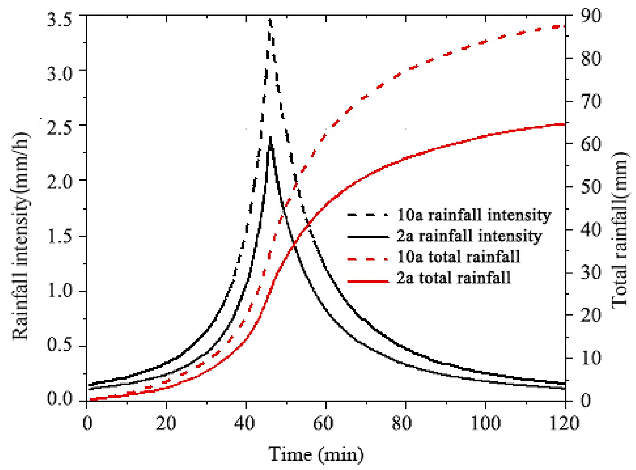
- Zhang, L.; Li, J.; Pei, H.; He, G. Analysis of rainfall patterns of short duration rainstorm in Nanjing. In Advances in Meteorological Science and Technology; China Meteorological Administration Training Center: Beijing, China, 2019; Volume 9, p. 3. [Google Scholar]
- Nigussie, T.A.; Altunkaynak, A. Modeling the effect of urbanization on flood risk in Ayamama Watershed, Istanbul, Turkey, using the MIKE 21 FM model. Nat. Hazards 2019, 99, 1031–1047. [Google Scholar] [CrossRef]


| Case Number | Terrain Resolution | Representation Method | Rainfall Intensity Return Periods | |
|---|---|---|---|---|
| Reference Cases | C1 | 17 m | BB + RD | 10 years |
| C2 | 17 m | BB + RD | 2 years | |
| Contrast Cases | C3 | 35 m | BB + RD | 10 years |
| C4 | 70 m | |||
| C5 | 35 m | BB + RD | 2 years | |
| C6 | 70 m | |||
| C7 | 17 m | RD | 10 years | |
| C8 | BB | |||
| C9 | 17 m | RD | 2 years | |
| C10 | BB |
| Simulation | Categories | |
|---|---|---|
| Inundation Depth (h) | Inundation Area (S) | |
| Reference case (RC) | ||
| Contrast case (CC) | ||
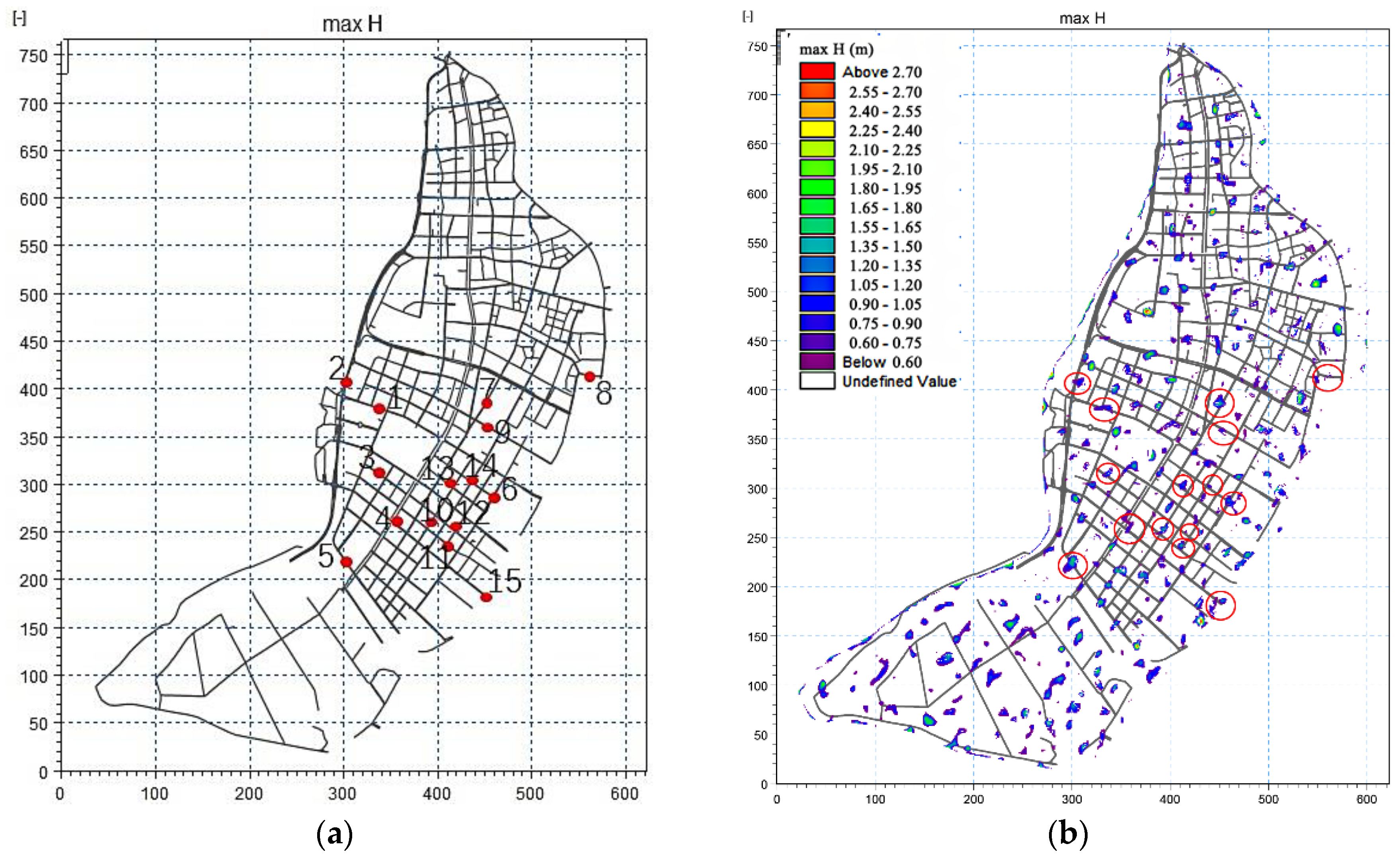
| No. | Inundation Positions |
|---|---|
| 1 | Mengdu street |
| 2 | South of Aoti new city tunnel, Yangzi river avenue |
| 3 | Fuchunjiang west street Nanxijiang street |
| 4 | Bailongjiang street |
| 5 | Jinshajiang street |
| 6 | Taishan Road |
| 7 | Xinglong street |
| 8 | Jiqingmen street to Changhong road from west to east |
| 9 | Yikang street to Lushan road |
| 10 | Hengshan road |
| 11 | Songshan road |
| 12 | Fuchunjiang street |
| 13 | Xin’anjiang street |
| 14 | Mudanjiang street |
| 15 | Shazhou police station |
| Rainfall Return Periods | Indicator | 70 m | 35 m | 17 m | 17 m |
|---|---|---|---|---|---|
| BB + RD Method | BB + RD Method | RD Method | BB Method | ||
| 2 years | RDA | 0.9896 | 0.9942 | 0.8978 | 0.9405 |
| RAA | 0.7623 | 0.9080 | 0.9538 | 0.9880 | |
| 10 years | RDA | 0.4905 | 0.8005 | 0.9266 | 0.9700 |
| RAA | 0.5669 | 0.8632 | 0.9449 | 0.9926 |
Publisher’s Note: MDPI stays neutral with regard to jurisdictional claims in published maps and institutional affiliations. |
© 2020 by the authors. Licensee MDPI, Basel, Switzerland. This article is an open access article distributed under the terms and conditions of the Creative Commons Attribution (CC BY) license (http://creativecommons.org/licenses/by/4.0/).
Share and Cite
Geng, Y.; Zhu, B.; Zheng, X. Effect of Independent Variables on Urban Flood Models. Water 2020, 12, 3442. https://doi.org/10.3390/w12123442
Geng Y, Zhu B, Zheng X. Effect of Independent Variables on Urban Flood Models. Water. 2020; 12(12):3442. https://doi.org/10.3390/w12123442
Chicago/Turabian StyleGeng, Yanfen, Baohang Zhu, and Xin Zheng. 2020. "Effect of Independent Variables on Urban Flood Models" Water 12, no. 12: 3442. https://doi.org/10.3390/w12123442
APA StyleGeng, Y., Zhu, B., & Zheng, X. (2020). Effect of Independent Variables on Urban Flood Models. Water, 12(12), 3442. https://doi.org/10.3390/w12123442